Robust High-Precision Time Synchronization for Distributed Sensor Systems in Challenging Environments

Highlights

What are the main findings?

• A novel DSTS architecture was proposed, integrating Bayesian filtering with DDPG reinforcement learning to solve synchronization in Challenging environments.
• The DSTS architecture achieved a final frequency synchronization precision of $4\times {10}^{-10}$ and a phase precision of $5\times {10}^{-10}$ s.

What are the implications of the main findings?

• The fusion of ToF and CIR data via Bayesian filtering provides an effective method to address non-linear communication errors and propagation path state uncertainty.
• The use of a DDPG agent as an “attention-like” mechanism is a viable strategy for managing network heterogeneity.

Abstract

Timing and time synchronization are critical capabilities of Global Navigation Satellite Systems (GNSSs), but their performance deteriorates significantly in challenging environments like urban canyons and tunnels. To address this issue, this paper proposes the Distributed Sensor Time Synchronization architecture (DSTS), a novel architecture integrating Bayesian filtering with deep reinforcement learning. DSTS utilizes Bayesian filtering to fuse Time-of-Flight (ToF) measurements with Channel Impulse Response features for real-time compensation of non-linear errors and accurate path state prediction. Concurrently, the Deep Deterministic Policy Gradient (DDPG) algorithm trains each node into an intelligent agent that dynamically learns optimal synchronization weights based on local information like neighbor clock stability and link quality. This allows the architecture to adaptively amplify reliable nodes while mitigating the negative effects of unstable peers and adverse channels, ensuring high accuracy and availability. Simulation experiments based on a real-world UWB dataset demonstrate the architecture’s exceptional performance. The Bayesian filtering module effectively mitigates non-linear errors, reducing the standard deviation of ToF measurements in NLOS scenarios by up to 51.6% (over 41.2% consistently) while achieving high path state prediction accuracy (>85% static, >95% simulated dynamic). In simulated dynamic and heterogeneous networks, the DDPG algorithm achieves a synchronization accuracy better than traditional average-consensus algorithms, ultimately reaching a frequency and phase precision of $4\times {10}^{-10}$ and $5\times {10}^{-10}$ s, respectively.

1. Introduction

High-precision timing and time synchronization are core capabilities provided by Global Navigation Satellite Systems (GNSSs), forming the foundation for applications such as target localization and tracking, multi-sensor data fusion, and change detection in the field of remote sensing [1,2,3]. Currently, the overall timing accuracy of GNSS products can reach <1 ns [4], but in complex or GNSS-denied environments such as urban canyons, tunnels, and indoor spaces, the performance of GNSS deteriorates significantly. This introduces a new requirement: ensuring that robust, high-precision time synchronization can still be maintained among distributed nodes in challenging environments. To ensure the continuity of clock synchronization, academia and industry commonly employ methods such as improving hardware, network synchronization protocols, and optimizing time information transfer to compensate for the limitations of GNSS.

In terms of hardware platforms for addressing challenging environments, researchers have utilized higher-resolution Wireless Communication Technologies. Dongare et al. utilized wide-spectrum UWB technology, designing the Pulsar platform to achieve 10-nanosecond level synchronization accuracy [5]. Building on this, Xue et al. further proposed a two-way handshake calibration mechanism to optimize the protocol against channel uncertainty, thereby improving synchronization robustness [6]. However, these methods do not account for the non-linear noise present in wireless communication, and their experiments were all conducted in LOS environments.

In terms of network communication protocols, traditional network-dependent methods like the Network Time Protocol (NTP) and the Precision Time Protocol (PTP) [7] rely on stable network infrastructure, making them often unsuitable for applications operating without external infrastructure, such as emergency management and environmental monitoring. Furthermore, their (millisecond- to sub-microsecond-level) synchronization accuracy cannot meet the demands of high-precision remote sensing platforms [8]. Based on this, researchers have proposed various consensus-based protocols. For instance, the Flooding Time Synchronization Protocol (FTSP) achieves network-wide synchronization by periodically broadcasting messages; a root node is elected to maintain and distribute a global time, which can provide microsecond-level accuracy suitable for simple networks [9]. The Reference Broadcast Synchronization (RBS) protocol enables relative time synchronization, also at the microsecond level, by having nodes exchange their local reception times of a common reference broadcast [10]. Scholars have recently studied distributed consensus time synchronization. Maggs et al. introduced Consensus Clock Synchronization, a protocol that achieves internal synchronization to a “virtual consensus clock” without a master node. It uses a two-stage approach: offset compensation via a “confidence-weighted running average”, and skew compensation, achieved by nodes observing their accumulated offset drift between rounds. This method was shown to reduce the standard deviation of clock errors from 387.6 to 10.75 clock ticks in simulations [11]. For UAVs in GNSS-denied settings, Gu et al. proposed a distributed “closed-loop clock tuning” framework. This method uses Synchronous Two-Way Ranging and a Kalman filter to jointly estimate clock errors and relative distances. It then uses these estimates for physical “clock steering” to adjust the onboard oscillators, achieving high-precision, sub-nanosecond-level time synchronization [12]. More recently, Jin et al. developed the DATJ algorithm, a consensus-based approach based on average consensus theory that does not require a reference node. It uniquely leverages both Doppler and timestamp information to jointly estimate clock skew and offset, achieving bounded convergence in highly dynamic conditions where traditional consensus methods fail [13].

In terms of communication, Wang et al. proposed a novel Time-Difference-of-Arrival TDOA-based joint synchronization and localization algorithm. Utilizing a “blink” model where anchors broadcast sequentially, the algorithm first estimates relative anchor clock skews using Least Squares Estimation (LSE) on TDOA differences between rounds, effectively canceling out the unknown distance terms. Subsequently, it employs Maximum Likelihood Estimation with skew-compensated biased Time-of-Flight (TOF) data to determine the relative positions of the anchors, followed by LSE to estimate relative clock offsets using the derived positions and skews. Once anchors are synchronized and relatively located, a tag can be positioned using MLE based on compensated TDOAs obtained from a single tag transmission. This approach achieves accurate synchronization and localization without requiring prior knowledge of anchor locations, demonstrating robustness against anchor position uncertainty and outperforming comparable methods in such scenarios [14].

Based on the research discussed above, the following issues still exist in challenging environments:

• Communication Error: In wireless synchronization, the communication channel is inherently non-ideal [8]. The non-linear characteristics prevalent in wireless communication systems—stemming from factors such as the complexity of signal propagation paths, environmental interference, and noise—frequently cause fluctuations in system performance, thereby impeding the achievement of high-precision time synchronization [15]. Specifically, these nonlinearities can arise from various sources, including but not limited to Non-Line-of-Sight (NLOS) occlusion, signal interference, noise, and changes in environmental conditions [16]. For example, existing research [17,18,19] has indicated that when a UWB communication system operates under NLOS conditions obstructed by a flipchart, the communication error fluctuates within a 5 ns range, with a standard deviation of 1 ns. However, the aforementioned studies all assume ideal communication conditions, ignoring the impact of communication errors on time synchronization accuracy.
• Clock Heterogeneity: Multi-source remote sensing platforms typically consist of diverse nodes that employ different clock sources, such as chip-scale atomic clocks or crystal oscillators. These sources exhibit varying degrees of clock stability. When current wireless synchronization methods are applied, the clock of the entire platform often synchronizes to the stability level of the least stable node, causing the overall platform clock to drift and fluctuate according to this inferior clock [20,21].
• Robustness: Almost all existing time synchronization algorithms are designed based on the assumption of homogeneous nodes, stable communication links, and relatively ideal environments [8]. However, during real-world deployment, environmental dynamics often introduce unpredictable errors. Given that the stability of the clock signal is of paramount importance to the entire system, the robustness of the synchronization algorithm becomes especially critical [22].

Building upon the platform presented in Pulsar [5], to address the issues mentioned above, this paper proposes the DSTS architecture. This architecture is designed to achieve high-precision time synchronization for multi-sensor platforms, particularly in challenging and denied environments where GNSSs fail. The architecture consists of a front-end and a back-end. The front-end utilizes UWB sensor and various clock sources, such as chip-scale atomic clocks and crystal oscillators, to acquire local clock data and measurements of frequency and time differences relative to neighboring nodes. The back-end then employs Bayesian filtering to perform real-time optimization of the Time of Flight in communications with these neighbors, thereby reducing the impact of communication errors on time synchronization. Concurrently, using the DDPG algorithm [23] to optimize network communication protocols, the architecture dynamically adjusts the synchronization weights assigned to different neighboring nodes. This optimizes synchronization accuracy when dealing with heterogeneous clock inputs and enhances the overall robustness of the time synchronization architecture.

The main contributions of this work are summarized as follows:

• Synchronization Architecture - DSTS: We propose the Distributed Sensor Time Synchronization Architecture, which integrates Bayesian filtering and DDPG to achieve robust, high-precision time synchronization in challenging, GNSS-denied environments.
• Real-Time Non-Linear Error Mitigation: We introduce a Bayesian filtering module that dynamically fuses ToF measurements with Channel Impulse Response (CIR) features to accurately estimate the true ToF and propagation path state (LOS/NLOS), effectively compensating for non-linear communication errors in real-time.
• Adaptive Synchronization Strategy via Reinforcement Learning: We leverage the DDPG algorithm to train each node as an intelligent agent capable of learning an optimal, adaptive synchronization policy. This agent dynamically adjusts synchronization weights based on local observations, enabling the architecture to intelligently manage clock heterogeneity and dynamic network conditions by prioritizing reliable information sources.
• Validated High Performance: Through simulations utilizing a real-world UWB dataset, we demonstrate that DSTS significantly outperforms traditional methods like Average Consensus, achieving frequency ($4\times {10}^{-10}$) and phase ($5\times {10}^{-10}$ s) precision.

The remainder of this paper is organized as follows. Section 2 provides a detailed description of the proposed DSTS architecture, including the design of the Bayesian filtering module and the DDPG based decision-making agent. Section 3 presents a series of extensive simulation experiments to validate the performance, adaptability, and robustness of our method. Section 4 discusses the broader implications and inherent limitations of our approach. Finally, Section 5 concludes this paper.

2. Architecture Design

The platform in [5] employs a two-way synchronization mechanism [24], as shown in Figure 1. It is commonly assumed that the nodes can transmit and receive at the same time. The ultimate goal of time synchronization is to achieve consistency in both frequency f and phase c.

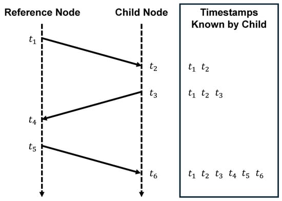
Figure 1. The bidirectional communication mechanism in a time synchronization architecture.

As shown in Figure 1, an illustration of the two-way communication between a reference node j and a subordinate node i, node i acquires three transmission timestamps $t_1,t_3,t_5$ and three reception timestamps $t_2,t_4,t_6$. The Time of Flight $T_{ij}$, frequency difference $\Delta f_{ij}$, and uncorrected phase difference $\Delta c_{ij}^{\prime }$ between the two nodes can be expressed as follows:

$$T_{ij}={\displaystyle \frac{(t_4-t_1)(t_6-t_3)-(t_3-t_2)(t_5-t_4)}{(t_4-t_1)+(t_6-t_3)+(t_3-t_2)+(t_5-t_4)}}+\epsilon$$

(1)

$$\Delta f_{ij}=f_i-f_j=(t_6-t_2)-(t_5-t_1)$$

(2)

$$\Delta c_{ij}^{\prime }=t_2-t_1$$

(3)

where $\epsilon$ represents the error introduced by factors such as the multipath effect. When an arbitrary node i exchanges timing information with its d adjacent nodes, it obtains the sets $T_i=\{T_{i1},T_{i2},\cdots ,T_{id}\}$, $F_i=\{\Delta f_{i1},\Delta f_{i2},\cdots ,\Delta f_{id}\}$ and $C_i^{\prime }=\{c_{i1}^{\prime },c_{i2}^{\prime },\cdots ,c_{id}^{\prime }\}$. As can be inferred from the two-way communication, the uncorrected phase offset $c_{ij}^{\prime }$ does not account for the communication propagation time [8]. Therefore, the true phase difference, $c_{ij}$, should be expressed as:

$$c_{ij}=\Delta c_{ij}^{\prime }-T_{ij}$$

(4)

This yields the set of corrected phase differences $C_i=\{c_{i1},c_{i2},\cdots ,c_{id}\}$. Subsequently, the node adjusts its own clock by computing and applying a compensation value.

The primary contribution of this paper is to enhance the robustness of the overall time synchronization architecture. This is achieved first by employing Bayesian filtering to obtain more accurate $T_i$ and to predict the current propagation path state, distinguishing between LOS and NLOS conditions. Concurrently, we utilize reinforcement learning to handle outliers within $\Delta F_i$ and $\Delta C_i$ sets, thereby improving the robustness of the entire architecture.

2.1. Architecture Overview

In this study, for a network comprising N nodes, the architecture at each node is divided into a front end and a back end, as shown in Figure 2. The front end primarily consists of a UWB communication device and a clock source. Through a bidirectional communication mechanism, the front end acquires measurements of the $T_i$, $\Delta F_i$, and $\Delta C_i^{\prime }$ from adjacent nodes. Concurrently, during the communication process, the front end UWB device obtains in real-time the maximum CIR for each received data packet, denoted as the set $P_i=\{P_{i1},P_{i2},\cdots ,P_{id}\}$. This parameter describes the maximum energy of the signal after it has propagated through the channel. Furthermore, the front end maintains an array to store the frequency values of its various neighboring nodes $\{f_1,f_2,\cdots ,f_d\}$, and calculates the frequency stability of these neighbors ${\sigma }_i=\{{\sigma }_1,{\sigma }_2,\cdots ,{\sigma }_d\}$. Ultimately, the front end transmits all the acquired data—the ToF values $T_i$, frequency differences $\Delta F_i$, uncorrected phase differences $\Delta C_i^{\prime }$, maximum CIR values $P_i$, and neighboring node frequency stabilities ${\sigma }_i$—to the back nd for further processing and analysis.

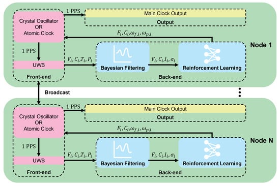
Figure 2. An overview of the DSTS architecture.

The back end is composed of a Bayesian filtering module and a DDPG algorithm. The core functions of the Bayesian filtering module include ToF value correction and the prediction of LOS and NLOS states. By integrating the measured $T_i$, with $P_i$, this module provides real-time corrected ToF values ${\widehat{T}}_i$, and estimates the propagation path state $l\in \{LOS,NLOS\}$. Based on the corrected ToF values, the uncorrected phase differences are further adjusted to obtain the accurate phase differences. The DDPG algorithm then dynamically adjusts the synchronization weights, $\alpha =\{{\alpha }_{i1},{\alpha }_{i2},\cdots ,{\alpha }_{id}\}$ and $\beta =\{{\beta }_{i1},{\beta }_{i2},\cdots ,{\beta }_{id}\}$, based on the frequency differences, the corrected phase differences, the propagation path state, and the neighboring node frequency stability. Using the following formula, the algorithm outputs the final frequency and phase correction values for node i:

$$F_i={\displaystyle \frac{{\alpha }_i\ast \Delta F_i}{d}}={\displaystyle \frac{{\alpha }_{i1}\ast \Delta F_{i1}+{\alpha }_{i2}\ast \Delta F_{i2}+\cdots +{\alpha }_{id}\ast \Delta F_{id}}{d}}$$

(5)

$$C_i={\displaystyle \frac{{\beta }_i\ast \Delta C_i}{d}}={\displaystyle \frac{{\beta }_{i1}\ast \Delta C_{i1}+{\beta }_{i2}\ast \Delta C_{i2}+\cdots +{\beta }_{id}\ast \Delta C_{id}}{d}}$$

(6)

2.2. A Bayesian Filtering Approach for ToF Error Mitigation

To address the issue of non-linear measurement errors introduced by challenging communication environments, such as multipath effects, in wireless time synchronization systems, this paper proposes a joint estimation algorithm based on mixed-state Bayesian filtering. This algorithm establishes a unified probabilistic inference framework to jointly estimate and dynamically track the true ToF value and the propagation path state. Through the online fusion of raw ToF measurement data with key statistical features extracted from the CIR, the proposed algorithm can effectively identify and provide real-time compensation for the systematic bias caused by NLOS propagation. This process significantly enhances the accuracy and robustness of the ToF estimation.

2.2.1. Hybrid State-Space Model

In this paper, the architecture state for node i at a discrete time instant t is defined as a mixed-state vector ${\mathit{x}}_{\mathit{i}}^{\mathit{t}}=\{T_i^t,l_i^t\}$, which comprises two components:

• The ToF Value $T_i^t$: A continuous variable representing the true Time-of-Flight of the target at time t. The prior estimate is denoted by ${\dot{T}}_i^t$, the measured value by $T_i^t$, and the posterior estimate by ${\widehat{T}}_i^t$.
• The Propagation Path State $l_i^t$: A discrete variable used to characterize the signal’s propagation mode. Its state space is $l_i^t\in \{LOS,NLOS\}$, representing Line-of-Sight and Non-Line-of-Sight propagation.

At any given time t, the architecture’s observation vector is ${\mathit{z}}_{\mathit{i}}^{\mathit{t}}=\{T_i^t,P_i^t\}$, and the history of all observations up to time t is $Z_i^t=\{{\mathit{z}}_{\mathit{i}}^{\mathbf{1}},{\mathit{z}}_{\mathit{i}}^{\mathbf{2}},\cdots ,{\mathit{z}}_{\mathit{i}}^{\mathit{t}}\}$. The observation vector contains two types of information extracted from the received signal: the ToF measurement and a CIR feature value.

The joint state of the architecture can be represented by a two-dimensional probability distribution, with the posterior probability given by $p({\mathit{x}}_{\mathit{i}}^{\mathit{t}}|Z_i^t)$. The state transition equation is as follows:

$$p({\mathit{x}}_{\mathit{i}}^{\mathit{t}}|Z_i^{t-1})=p({\mathit{x}}_{\mathit{i}}^{\mathit{t}}|{\mathit{x}}_{\mathit{i}}^{\mathit{t}-\mathbf{1}})·p({\mathit{x}}_{\mathit{i}}^{\mathit{t}-\mathbf{1}}|Z_i^{t-1})$$

(7)

According to Bayesian filtering theory, the transition of the state ${\mathit{x}}_{\mathit{i}}^{\mathit{t}}$ is assumed to adhere to the Markov process assumption; that is, the current state ${\mathit{x}}_{\mathit{i}}^{\mathit{t}}$ depends solely on the preceding state ${\mathit{x}}_{\mathit{i}}^{\mathit{t}-\mathbf{1}}$.

The other critical component of the filtering algorithm is the observation model. This model defines the probability of obtaining a specific observation ${\mathit{z}}_{\mathit{i}}^{\mathit{t}}$ given the current true state ${\mathit{x}}_{\mathit{i}}^{\mathit{t}}$. To construct this model, we analyzed the statistical characteristics of observations under different propagation path states (LOS/NLOS) using a large set of prior experimental data [17]. We first built empirical frequency histograms and then converted them into conditional probability density functions using a non-parametric kernel density estimation method.

2.2.2. Prediction Step: Prior Calculation

The prediction step of the Bayesian filter aims to derive the prior probability of the architecture state at the current time t, $p({\dot{\mathit{x}}}_{\mathit{i}}^{\mathit{t}}|Z_i^{t-1})$, based on the posterior probability from the previous time step $p({\widehat{\mathit{x}}}_{\mathit{i}}^{\mathit{t}-\mathbf{1}}|Z_i^{t-1})$. Based on the assumption that the states $T_i^t$ and $l_i^t$ are mutually independent, the joint state transition model can be decomposed into the product of two independent models:

$$p({\dot{\mathit{x}}}_{\mathit{i}}^{\mathit{t}}|{\widehat{\mathit{x}}}_{\mathit{i}}^{\mathit{t}-\mathbf{1}})=p({\dot{T}}_i^t|{\widehat{T}}_i^{t-1})·P(l_i^t|l_i^{t-1})$$

(8)

This allows for the probability distributions of the ToF and the propagation path state to be calculated separately.

For the dynamic prediction of the true ToF value, we employ a Gaussian random walk model to describe its evolution. This model assumes that the true ToF at the current time is the value from the previous time step plus a zero-mean Gaussian process noise. The transition probability $p({\dot{T}}_i^t|{\widehat{T}}_i^{t-1})$ is implemented through a convolution with a Gaussian kernel.

$$p({\dot{T}}_i^t|Z_i^{t-1})=\int p({\dot{T}}_i^t|{\widehat{T}}_i^{t-1})·p({\widehat{T}}_i^{t-1}|Z_i^{t-1})d{\widehat{T}}_i^{t-1}$$

(9)

The evolution of the propagation path state $l_i^t$ is modeled as a discrete-time Markov chain. The state transition can be defined by a $2\times 2$ state transition matrix:

$$p({\dot{l}}_i^t|{\widehat{l}}_i^{t-1})=\left[\begin{array}{cc}\mu & 1-\mu \\ 1-\mu & \mu \end{array}\right]$$

(10)

where $\mu$ represents the probability of the scene remaining unchanged. The prior probability distribution for the path state is obtained by multiplying the posterior probability vector from the previous time step with this transition matrix.

$$p({\dot{l}}_i^t|Z_i^{t-1})=p({\dot{l}}_i^t|{\widehat{l}}_i^{t-1})·p({\widehat{l}}_i^{t-1}|Z_i^{t-1})$$

(11)

By combining these two independent prediction processes, the joint prior probability distribution of the architecture at time t can be expressed as the product of the two independent predicted distributions, yielding the final joint predictive prior distribution.

$$p({\widehat{\mathit{x}}}_{\mathit{i}}^{\mathit{t}}|Z_i^t)=p({\mathit{x}}_{\mathit{i}}^{\mathit{t}}|{\mathit{z}}_{\mathit{t}},Z_i^{t-1})\propto p({\mathit{z}}_{\mathit{i}}^{\mathit{t}}|{\mathit{x}}_{\mathit{i}}^{\mathit{t}})·p({\dot{\mathit{x}}}_{\mathit{i}}^{\mathit{t}}|Z_i^{t-1})$$

(12)

2.2.3. Update Step: Posterior Calculation

When the node acquires a new observation vector ${\mathit{z}}_{\mathit{i}}^{\mathit{t}}$, at time t, the update step utilizes this information to refine the prior probability distribution $p({\dot{\mathit{x}}}_{\mathit{i}}^{\mathit{t}}|{\mathit{z}}_{\mathit{i}}^{\mathit{t}-\mathbf{1}})$, into the posterior probability distribution $p({\widehat{\mathit{x}}}_{\mathit{i}}^{\mathit{t}}|{\mathit{z}}_{\mathit{i}}^{\mathit{t}})$. According to Bayes’ theorem, this process requires the definition of an observation model, which is the joint likelihood function:

$$p({\widehat{\mathit{x}}}_{\mathit{i}}^{\mathit{t}}|Z_i^t)=p({\mathit{x}}_{\mathit{i}}^{\mathit{t}}|{\mathit{z}}_{\mathit{t}},Z_i^{t-1})\propto p({\mathit{z}}_{\mathit{i}}^{\mathit{t}}|{\mathit{x}}_{\mathit{i}}^{\mathit{t}})·p({\dot{\mathit{x}}}_{\mathit{i}}^{\mathit{t}}|Z_i^{t-1})$$

(13)

where $p({\mathit{z}}_{\mathit{i}}^{\mathit{t}}|{\mathit{x}}_{\mathit{i}}^{\mathit{t}})$ is the measurement likelihood function. Assuming that the measurement value $T_i^t$ and the CIR feature $P_i^t$ are mutually independent given the true state ${\mathit{x}}_{\mathit{i}}^{\mathit{t}}$, we must separately compute the propagation path state likelihood $p({\mathit{z}}_{\mathit{i}}^{\mathit{t}}|{\widehat{l}}_i^t)$ and the ToF likelihood $p({\mathit{z}}_{\mathit{i}}^{\mathit{t}}|{\widehat{T}}_i^t,{\widehat{l}}_i^t)$.

The propagation path state likelihood $p({\mathit{z}}_{\mathit{i}}^{\mathit{t}}|{\widehat{l}}_i^t)$ describes the conditional probability between the CIR feature and the propagation path state. This likelihood value is obtained directly by looking up the value in the non-parametric probability density function models for LOS and NLOS scenarios, which were constructed in Section 2.2.1.

The ToF likelihood $p({\mathit{z}}_{\mathit{i}}^{\mathit{t}}|{\widehat{T}}_i^t,{\widehat{l}}_i^t)$ is used to describe the probabilistic relationship between the measured value $T_i^t$ and the true value ${\widehat{T}}_i^t$, a relationship that is influenced by the path state $l_i^t$. The algorithm models this using a Gaussian distribution, which characterizes the distribution of the measurement $T_i^t$ around the true ToF value for a given condition. The likelihoods for the LOS and NLOS scenarios are calculated separately:

$$p(T_i^t|P_i^t,l_{LOS})=\mathcal{N}(T_i^t,{\mu }_i,{\sigma }_{LOS})$$

(14)

$$p(T_i^t|P_i^t,l_{NLOS})=\mathcal{N}(T_i^t,{\mu }_i,{\sigma }_{NLOS})$$

(15)

The mean of the Gaussian distribution, ${\mu }_i$ is pre-calibrated from the frequency histograms detailed in Section 2.2.1, while the standard deviation, $\sigma$, is the noise standard deviation for the current LOS or NLOS condition.

The final posterior probability can then be expressed as follows:

$$p({\widehat{\mathit{x}}}_{\mathit{i}}^{\mathit{t}}|Z_i^t)=p({\mathit{z}}_{\mathit{i}}^{\mathit{t}}|{\mathit{x}}_{\mathit{i}}^{\mathit{t}})·p({\dot{\mathit{x}}}_{\mathit{i}}^{\mathit{t}}|Z_i^t)$$

(16)

From the posterior probability distribution $p({\widehat{\mathit{x}}}_{\mathit{i}}^{\mathit{t}}|Z_i^t)$, the probability estimate of the propagation path state $p({\widehat{l}}_i^t|Z_i^t)$ can be obtained by marginalizing over the ToF dimension ${\widehat{T}}_i^t$. The ToF estimate ${\widehat{T}}_i^t$ is calculated by computing the conditional expectation of the posterior distribution:

$$E[{\widehat{T}}_i^t|l_i^t,Z_i^t]=\int {\widehat{T}}_i^{t}p(l_i^t,Z_i^t)d{\widehat{T}}_i^t$$

(17)

This process yields the Bayesian-filtered ToF estimate, which is subsequently used to obtain the corrected phase difference set $\Delta C_i$.

The complete procedure for the Bayesian filtering algorithm is summarized in Algorithm 1.

Algorithm 1: Bayesian Filtering for ToA and Propagation Path State Estimation

2.3. A DDPG Distributed Clock Synchronization Algorithm

Traditional clock synchronization methods often struggle to adapt to the dynamic environmental changes and communication topology heterogeneity inherent in multi-sensor remote sensing platform deployments. An ideal distributed synchronization algorithm must be capable of making fine-grained decisions in a continuous space to output precise, non-discrete control parameters. Furthermore, it must exhibit high sample efficiency to learn effectively from communication interactions, which are metabolically expensive.

To address these challenges, this paper proposes a distributed clock synchronization algorithm based on the Deep Deterministic Policy Gradient. The structure of the algorithm is illustrated in Figure 3. The core idea, which borrows from the Attention Mechanism, enables each node to adaptively amplify the influence of important neighbors while disregarding minor or anomalous ones, thereby achieving robust synchronization in dynamic network environments. Similarly to how attention mechanisms learn dynamic weights to focus on critical information, our algorithm trains each network node to act as an independent intelligent agent. Through reinforcement learning, this agent autonomously generates a set of weighting coefficients used to perform a weighted aggregation of clock information from its neighbors. Moreover, the algorithm’s off-policy nature, combined with an experience replay mechanism, allows the agent to learn from historical data, ensuring high sample efficiency. To further stabilize the training process and strike a balance between exploration and exploitation, we have optimized the algorithm’s exploration logic. This section will provide a detailed exposition of this reinforcement learning paradigm, including the formulation of the Markov Decision Process and the specific implementation of the DDPG algorithm.

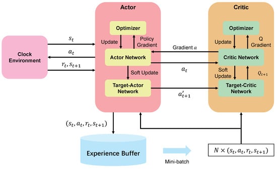
Figure 3. An overview of the DDPG algorithm.

2.3.1. Markov Decision Process

We formulate the distributed clock synchronization problem for each individual node as a Markov Decision Process (MDP). In our setting, every node $i\in \{1,2,\dots ,N\}$ within the network acts as an independent learning agent, making decisions based on its local observations without requiring any global information. The MDP is formally defined by the five-tuple $\{S,A,P,R,\gamma \}$, where S denotes the state space, A represents the action space, R is the reward function, P is the state transition probability, and $\gamma$ is the discount factor. As our proposed algorithm learns model-free directly through interaction with the environment, it is not necessary to explicitly model the state transition probability P.

State Space (S): At any given time step t, the state of agent i, ${\mathit{s}}_{\mathit{i}}^{\mathit{t}}\in S$, is defined as a feature vector formed by concatenating the interaction information from all of its d neighboring nodes. Specifically, this includes four key dimensions for each neighbor j: the frequency difference $\Delta f_{ij}$, the phase difference $\Delta c_{ij}$, the propagation path state $l_{ij}$ estimated by the Bayesian filter, and the neighbor’s frequency stability ${\sigma }_j$. The complete state vector can be represented as follows:

$${\mathit{s}}_{\mathit{i}}^{\mathit{t}}={[\Delta f_{i1}^t,\Delta c_{i1}^t,l_{i1}^t,{\sigma }_1^t,...,\Delta f_{id}^t,\Delta c_{id}^t,l_{id}^t,{\sigma }_d^t]}^T$$

(18)

The dimension of this state vector is $4\times d$. It serves as the input to both the Actor and Critic networks to enable policy learning and optimization based on local perception.

Action Space (A): The agent’s action space is designed to be continuous. At each time step t, the action of agent i, ${\mathit{a}}_{\mathit{i}}^{\mathit{t}}\in A$, is defined as a composite vector containing two sets of normalized weighting coefficients used to adjust its own clock:

$${\mathit{a}}_{\mathit{i}}^{\mathit{t}}=({\mathit{w}}_{p,i}^t,{\mathit{w}}_{f,i}^t)$$

(19)

where ${\mathit{w}}_{p,i}^t=\{w_{p,i1}^t,\cdots ,w_{p,id}^t\}$ and ${\mathit{w}}_{f,i}^t=\{w_{f,i1}^t,\cdots ,w_{f,id}^t\}$ are the weight vectors for frequency and phase adjustments, respectively. These weights are normalized such that $\sum w_{p,ij}=1$ and $\sum w_{f,ij}=1$.

Reward Function (R): The design of the reward function is critical for guiding the agent to learn the desired behavior. We have engineered a multi-objective composite function, which comprises the following three components, aimed at the simultaneous optimization of multiple synchronization metrics:

• High-Precision Synchronization Reward ($r_{\mathrm{sync}}$): This component is designed to incentivize the agent to maintain a minimal clock offset with its neighbors. We implement a tiered reward mechanism to encourage the agent to pursue progressively higher levels of synchronization accuracy. A base reward is granted when the absolute values of both the frequency difference and phase difference with a neighbor j are below a threshold ${\omega }_1$. An additional reward is given when these differences are below a more stringent high-precision threshold ${\omega }_2$. The formula is as follows:

  $$r_{\mathrm{sync}}=\sum _{j\in \lceil (i)}\mathbb{I}(|\Delta f_{ij},\Delta c_{ij}| <{\omega }_1)+\alpha ·\mathbb{I}(|\Delta f_{ij},\Delta c_{ij}|<{\omega }_2)$$

  (20)

  where $I()$ is the indicator function, and ${\omega }_1$ and ${\omega }_2$ are hyper-parameters representing the reward weights.
• Penalty for Unreliable Neighbors ($r_{\mathrm{robust}}$): This component acts as a penalty to guide the agent to actively identify and reduce its reliance on unstable clock sources. The agent receives a penalty if it assigns a high synchronization weight to a neighbor j whose clock stability is inferior to its own.
• Channel Quality Awareness Penalty ($r_{\mathrm{channel}}$): This is also a penalty term, which serves to compel the agent to be aware of the communication channel quality. The agent is penalized if it assigns a high weight to a neighbor currently under NLOS conditions. This encourages the agent to mitigate the risk of information distortion that can result from poor channel quality.

These three components work synergistically to guide the agent’s learning toward robust, high-precision synchronization. While $r_{\mathrm{sync}}$ provides primary positive reinforcement for achieving accuracy by minimizing differences with neighbors, the penalty components $r_{\mathrm{robust}}$ and $r_{\mathrm{channel}}$ act as crucial negative feedback mechanisms. They steer the agent away from incorporating potentially corrupting information from neighbors with unstable clocks or those communicating under NLOS conditions. This forces the agent to learn a strategy that balances the drive for precision (maximizing $r_{\mathrm{sync}}$) against the need for reliability (minimizing penalties). Consequently, the agent learns to prioritize and assign higher weights to neighbors that are both temporally close and demonstrably stable and communicate clearly, while down-weighting or ignoring neighbors that would compromise the overall architecture’s stability and accuracy.

The total reward for agent i at time step t is the summation of these three components:

$$r_i^t=r_{\mathrm{sync}}+r_{\mathrm{robust}}+r_{\mathrm{channel}}$$

(21)

2.3.2. Deep Deterministic Policy Gradient

This algorithm employs the Deep Deterministic Policy Gradient as its core reinforcement learning framework. DDPG is a model-free, off-policy algorithm based on an Actor–Critic architecture, which is commonly used to handle problems with continuous action spaces. In our distributed system, each node functions as an independent agent, maintaining its own dedicated set of Actor and Critic networks. To better meet the high-precision and high-stability demands of the time synchronization task, we have optimized the exploration strategy to achieve a more effective balance between exploration and exploitation.

The Actor Network is responsible for implementing a deterministic policy. It receives the state ${\mathit{s}}_{\mathit{i}}^{\mathit{t}}$ as input and deterministically outputs an action ${\mathit{a}}_{\mathit{i}}^{\mathit{t}}$, which corresponds to the set of weighting coefficients. This network is trained to directly maximize the expected cumulative reward. In our implementation, the Actor network consists of several Fully Connected Layers with ReLU activation functions. To ensure stability during the training process, we adopt a hybrid exploration strategy, which is expressed as follows:

$${\mathit{a}}_{\mathit{t}}=\left\{\begin{array}{cc}\mu (s_t|{\theta }^{\mu })\hfill & u>{ϵ}_t\hfill \\ \mu (s_t|{\theta }^{\mu })+{\mathcal{N}}_t\hfill & u\le {ϵ}_t\hfill \end{array}\right.$$

(22)

where $\mu$ is a random number sampled from a uniform distribution on the interval $[0,1]$, ${ϵ}_t$ is an exploration probability threshold that decays over time t, and ${\mathcal{N}}_t$ represents Gaussian exploration noise, the magnitude of which also decays as training progresses. The raw action parameters output by the Actor network are not applied directly. Instead, they undergo a normalization process to be converted into the final action, which satisfies the necessary constraints. This step ensures that the output weights for both phase and frequency are non-negative and that the sum of the weights for each category equals 1.

The Critic Network is designed to approximate the action-value function $Q({\mathit{s}}_{\mathit{i}}^{\mathit{t}},{\mathit{a}}_{\mathit{i}}^{\mathit{t}})$. Its task is to evaluate the long-term value of executing action ${\mathit{a}}_{\mathit{i}}^{\mathit{t}}$ in state ${\mathit{s}}_{\mathit{i}}^{\mathit{t}}$. It receives both the state and the action as a joint input and outputs a single scalar Q-value. To more effectively process these two inputs of different natures, the network architecture first passes the state vector and the action vector through separate input layers. The resulting feature vectors are then concatenated, and this combined representation is fed into subsequent fully connected layers to produce the final value estimation. The network’s structure is illustrated in Figure 4.

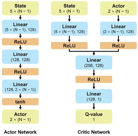
Figure 4. The network structure of the DDPG algorithm.

To break the temporal correlation between consecutive samples and improve data utilization, each agent is equipped with an experience replay buffer. This buffer stores historical experience tuples of the form $\{{\mathit{s}}_{\mathit{i}}^{\mathit{t}},{\mathit{a}}_{\mathit{i}}^{\mathit{t}},r_i^t,{\mathit{s}}_{\mathit{i}}^{\mathit{t}+\mathbf{1}}\}$. During training, the algorithm learns by sampling a random minibatch of data from this buffer.

The objective of the Critic Network update is to minimize the Mean Squared Bellman Error. Its loss function is defined as follows:

$$(L_C)={\displaystyle \frac{1}{N}}\sum _{i=1}^N\left[{\left(Q({\mathit{s}}_{\mathit{i}}^{\mathit{t}},{\mathit{a}}_{\mathit{i}}^{\mathit{t}}|{\theta }^Q)-y_i\right)}^2\right]$$

(23)

To ensure a stable learning process, the target value, $y_i$, is calculated using target networks. Specifically, the target Actor network, ${\mu }^{\prime }$, is used to select the optimal action for the next state, ${\mathit{s}}_{\mathit{i}}^{\mathit{t}+\mathbf{1}}$, and the target Critic network, $Q^{\prime }$, is used to evaluate the value of that state-action pair:

$$y_i=r_i^t+\gamma Q^{\prime }({\mathit{s}}_{\mathit{i}}^{\mathit{t}+\mathbf{1}},{\mu }^{\prime }({\mathit{s}}_{\mathit{i}}^{\mathit{t}+\mathbf{1}}|{\theta }^{{\mu }^{\prime }})|{\theta }^{Q^{\prime }})$$

(24)

The Actor Network is updated following the policy gradient method. Its goal is to generate actions that maximize the Q-value output from the Critic network. Therefore, the Actor’s parameters are updated by performing gradient ascent on the expected return. To further stabilize the training process, the parameters of the target networks are not copied directly from the main networks. Instead, they are updated iteratively using a soft update rule:

$${\theta }^{\prime }\leftarrow \tau \theta +(1-\tau ){\theta }^{\prime }$$

(25)

where $\tau$ is the update factor.

The operational logic of the algorithm is presented in Algorithm 2.

Algorithm 2: Decentralized Clock Synchronization

3. Experiments

In this section, we conduct extensive simulation studies on the aforementioned Bayesian filtering module, the DDPG algorithm, and the complete time synchronization system to evaluate their performance. The UWB data used in our experiments is sourced from [17]. This dataset was collected using Decawave DW1000 chip—the same hardware used in [5]—and contains ToF measurements obtained via a two-way measurement protocol. In addition to the final ToF values, the dataset includes intermediate measurement variables, maximum CIR data, and annotated occlusion states. The clock data is modeled as a normal distribution, $X\sim \mathcal{N}(\mu ,{\sigma }^2)$, based on a simplified model from [25].

The dataset used for the experiments covers measurements taken under two different distance conditions, 3 m and 5 m, and across various environments, including unobstructed, flipchart-obstructed, human body-obstructed, monitor-obstructed, and wood board-obstructed scenarios. In total, the dataset comprises 1.2 million data samples.

3.1. A Bayesian Filtering Experiment Results

To validate the performance of the proposed Bayesian filtering algorithm in scenarios simulating real-world conditions, we first classified and labeled the data to construct precise empirical probability density functions for the observation model.

• Model Calibration Dataset: This dataset comprises data from various distances under both LOS and NLOS (white board, human body, and monitor occlusions) scenarios. For each scenario combination, we acquired 300,000 raw ToF measurements (T) and CIR feature values (P). These data were used to build the algorithm’s likelihood function model as shown in Figure 5.
  

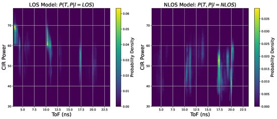  Figure 5. This figure presents the probability histogram of LOS and NLOS conditions.
• Algorithm Validation Dataset: For performance evaluation, we utilized completely independent test sequences, each containing 600 data points. These included four static scenarios and one dynamic scenario, which are detailed below.
• Model Parameter Settings: Based on the DW1000 chip’s datasheet and the noise characteristics of the test scenarios in the dataset, we set the noise standard deviation parameter for the ToF measurements as follows: 0.5 for LOS scenarios and 1.0 for NLOS scenarios.

We first evaluated the algorithm’s performance in four static environments, focusing on its propagation path state prediction accuracy and its ToF estimation precision. Prediction accuracy is defined as the proportion of samples for which the algorithm’s output path state matches the ground truth. ToF estimation precision is measured by comparing the standard deviation of the ToF values before filtering raw measurements against the standard deviation after filtering algorithm’s output.

The results of the algorithm are presented in Figure 6, with a summary provided in Table 1. The algorithm successfully identifies the correct propagation path state with high accuracy (over 85%) across all scenarios, achieving 100% accuracy in the LOS and monitor-occlusion environments. For all tested NLOS scenarios, the standard deviation of the ToF estimates, after being processed by our algorithm, was significantly lower than that of the raw measurements, with precision improvements ranging from 41.2% to 51.6%. This demonstrates that the algorithm can effectively suppress measurement noise and fluctuations in NLOS environments, thereby producing smoother and more reliable ToF estimates.

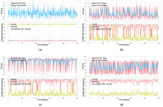
Figure 6. Illustration of the algorithm’s filtering performance. The top plot shows the measured ToF values and the corresponding filtered values at each time step. The bottom plot shows the probability of the current state being LOS or NLOS, as estimated by the algorithm at each time step: (a) 3 m, (LOS) (b) 3 m, flipchart (NLOS) (c) 5 m, human (NLOS) (d) 5 m, monitor (NLOS).

Table 1. This table shows the prediction and filtering performance of the algorithm in different environments.

Test Sequence	Path Accuracy	Raw ToF $\mathit{\sigma }$	Filtering ToF $\mathit{\sigma }$	$\mathit{\sigma }$ Promotion
3 m, - (LOS)	100%	-	-	-
3 m, Flipchart (NLOS)	84%	1.29	0.76	41.2%
5 m, Human (NLOS)	91.8%	0.91	0.44	51.6%
5 m, Monitor (NLOS)	100%	0.92	0.49	46.7%

To validate the algorithm’s adaptive capability in a dynamically changing environment, we designed a scenario that transitions from NLOS to LOS: the first 300 samples were collected with a flipchart occlusion at a 3 m distance, after which the obstruction was removed for the final 300 LOS samples. In this simulated dynamic test, the algorithm achieved an overall path state prediction accuracy of 95.68%, showcasing its capacity for rapid detection and correct identification of environmental changes. In terms of ToF estimation, the standard deviation for the entire measurement sequence was reduced from 1.20 to 0.96. The filtering process is depicted in Figure 7, which clearly illustrates the algorithm’s identification and judgment as the scene switches from NLOS to LOS.

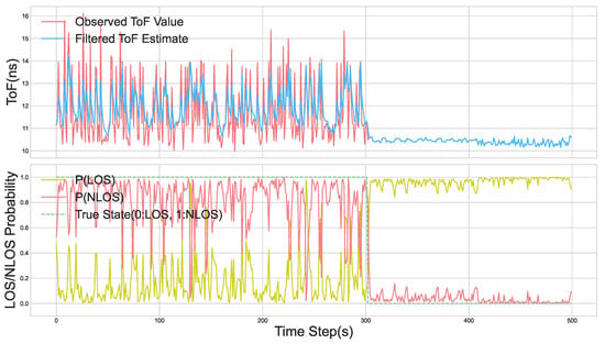
Figure 7. The top plot shows the measured ToF values and the corresponding filtered values at each time step. The bottom plot shows the probability of the current state being LOS or NLOS, as estimated by the algorithm at each time step.

The mixed-state Bayesian filtering algorithm proposed in this paper demonstrated excellent performance across multiple tests simulating real-world environments. The experimental results provide quantitative proof of the algorithm’s key capabilities: high-precision environmental perception, which means it can identify LOS/NLOS propagation paths with an accuracy exceeding 85%, and significant noise suppression, which means that, in various NLOS scenarios, the algorithm reduces the standard deviation of ToF measurements by more than 41.2%. This effectively smooths data fluctuations, thereby providing more precise and robust data for the subsequent clock offset calculations. Simultaneously, the simulated dynamic scenario test confirmed that this algorithm is not limited to static settings but can effectively track environmental changes.

3.2. DDPG Experiment Results

This section aims to evaluate the performance of our proposed DDPG algorithm in learning an adaptive synchronization strategy. The core of the experiment is to verify whether the agent can achieve high-precision distributed synchronization by learning dynamic weight allocation within a complex network characterized by heterogeneous clock sources.

We constructed a simulated network environment containing 10 nodes, with the connectivity topology illustrated in the corresponding Figure 8. The communication data used in the experiment was derived from the real-world UWB measurement dataset, which was processed and corrected using the Bayesian filtering method described in Section 3.1. After processing, a total of 2,000,000 data samples were generated. These samples were uniformly distributed across each connection in the topology, resulting in 100,000 data points per link.

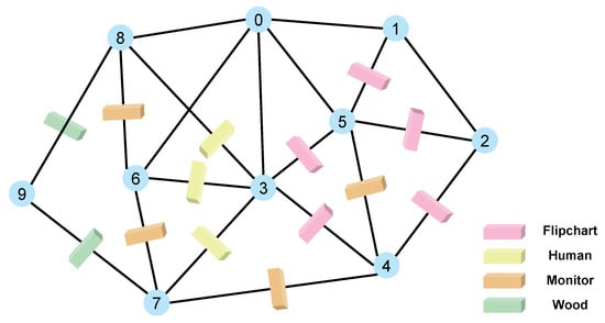
Figure 8. This figure shows the node connectivity diagram and illustrates the obstructions between nodes. The numbers in the figure represent node numbers.

3.2.1. Static Environment Experiment Results

To simulate the clock heterogeneity of real-world multi-sensor platforms, we assigned distinct frequency stability parameters to each of the 10 network nodes. The selection of these parameters was informed by the official manuals for commercial components such as crystal oscillators, chip-scale rubidium atomic clocks, and cesium atomic clocks, covering a stability range from ${10}^{-6}$ to ${10}^{-11}$, as detailed in Table 2 [25,26].

Table 2. This table lists the stability parameters for various clock sources.

Clock Type	Frequency Stability	Frequency Tuning Threshold
Crystal Oscillator	$2\times {10}^{-7}$∼$2\times {10}^{-6}$	$\pm 5\times {10}^{-5}$
Chip-Scale Rubidium Atomic Clock	≤$5\times {10}^{-11}$	$\pm 3\times {10}^{-9}$
Chip-Scale Cesium Atomic Clock	≤$1.5\times {10}^{-11}$	$\pm 3\times {10}^{-9}$

Specifically, in conjunction with our dataset, the frequency stability values assigned to the 10 nodes were set to the following sequence: [$2.678\times {10}^{-10}$, $1.178\times {10}^{-7}$, $1.122\times {10}^{-11}$, $1.093\times {10}^{-10}$, $6.482\times {10}^{-10}$, $2.303\times {10}^{-11}$, $2.141\times {10}^{-7}$, $1.52\times {10}^{-10}$, $3.345\times {10}^{-11}$, $2.324\times {10}^{-11}$]. Frequency drift was simulated using a Wiener process based on these frequency stabilities. This setup was intentionally designed to create a mixed environment containing both stable and unstable clock sources, allowing for a comprehensive evaluation of our algorithm’s adaptive capabilities.

The hyperparameters used for the DDPG algorithm are listed in Table 3.

Table 3. This table presents the hyperparameters set for the DDPG algorithm.

Parameter	Value
Episode Timesteps	500
Number of Episodes	200
Actor Learning Rate	${10}^{-4}$
Critic Learning Rate	${10}^{-3}$
Discount Factor	0.9
Batch Size	256
Replay Buffer Size	50,000
Soft update factor	0.005

As illustrated in Figure 9, the cumulative reward for each of the 10 agent nodes shows significant growth over the course of the training process. The plot indicates that the entire system converges to a stable and high level of reward after approximately 75 episodes. This demonstrates that all agents successfully learned an effective policy to maximize the multi-objective composite reward function that we designed.

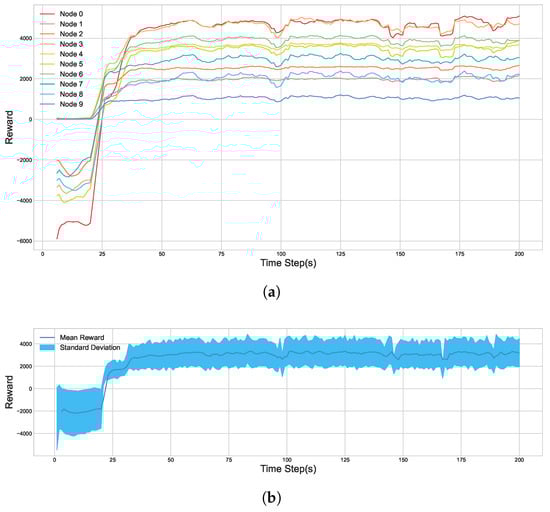
Figure 9. Node Reward Values in Static Environment. (a) The cumulative reward for each individual node. (b) The average cumulative reward for the entire system.

As shown in Figure 10, after the training converged, the frequency synchronization accuracy among the network nodes reached $\pm 4\times {10}^{-10}$, and the phase synchronization accuracy reached $\pm 8\times {10}^{-10}$ s, excluding the nodes that were identified as having poor performance. This indicates that the proposed DDPG algorithm can effectively address the challenge of clock heterogeneity and achieve high-precision distributed time synchronization.

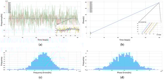
Figure 10. Time Synchronization Performance of the Algorithm. (a) Frequency synchronization across the system during the final episode. (b) Phase synchronization across the system during the final episode. (c) A histogram of the frequency differences for each node relative to the system’s average frequency over the last 300 time steps, excluding anomalous nodes. (d) A histogram of the phase differences for each node relative to the system’s average phase over the last 300 time steps, excluding anomalous nodes.

Figure 11 illustrates the evolution of the weights that Node 3 assigns to its neighboring nodes during the training process. It can be clearly observed from the plot that the weight Node 3 allocates to Node 6 ultimately converges to nearly zero. This action demonstrates that the agent, through learning, can actively identify and ignore unstable nodes within the network, thereby avoiding their adverse effects on its own clock.

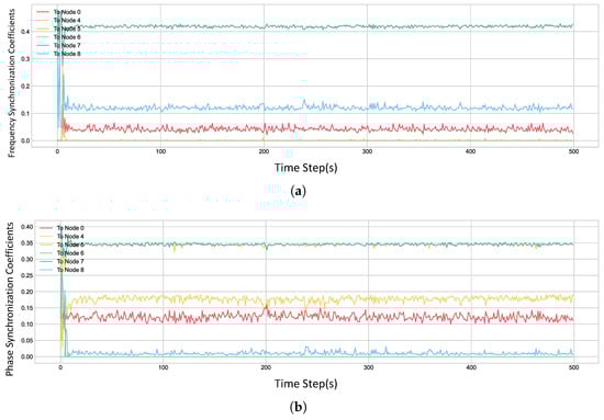
Figure 11. Real-time weight values output by the algorithm for Node 3. (a) The frequency weights. (b) The phase weights.

3.2.2. Simulated Dynamic Environment Experiment Results

To further evaluate the adaptability and robustness of the DSTS architecture in dynamically changing environments, we designed an experiment to simulate unexpected changes in node states, mirroring real-world conditions. The experiment comprises a total of 200 training episodes.

• Initial Stage (Episodes 1–100): The initial configuration of the experimental environment is identical to the static heterogeneous network described in Section 3.2.1.
• Abrupt Environmental Change (At Episode 100): At the beginning of the 100th episode, we introduce an abrupt change by instantaneously modifying the clock frequency stability parameters for all nodes in the network. The new stability sequence is set to [$2.678\times {10}^{-10}$, $1.178\times {10}^{-11}$, $1.122\times {10}^{-11}$, $1.093\times {10}^{-10}$, $1.482\times {10}^{-7}$, $2.303\times {10}^{-11}$, $2.141\times {10}^{-10}$, $1.524\times {10}^{-10}$, $3.345\times {10}^{-7}$, $2.324\times {10}^{-11}$], and frequency drift is simulated using a Wiener process based on these frequency stabilities. Under this new configuration, the worst-performing nodes in the network shift from the initial Node 1 and Node 6 to Node 4 and Node 8. Concurrently, to simulate a gradual global environmental drift, the stability of some of the other nodes also undergoes subtle evolution during the long-term training process.
• Adaptive Stage (Episodes 101–200): Following the environmental shift, we continue to train the agents, observing whether their policies can readjust to adapt to the new distribution of node stabilities.

As depicted in Figure 12, when the abrupt environmental change occurs at episode 100, there is a distinct and instantaneous drop in the average reward for all nodes. This indicates that the policy the agents learned based on the old environment is no longer optimal. However, the algorithm demonstrates its online learning capability; after a brief period of performance oscillation, the reward curve rapidly recovers and re-converges to a peak level comparable to that before the change, successfully adapting to the new environmental conditions.

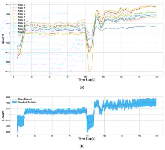
Figure 12. Node reward values in Simulated Dynamic Environment. (a) The cumulative reward for each individual node. (b) The average cumulative reward for the entire system.

This macroscopic performance recovery stems from the dynamic adjustment of the agents’ policies. Figure 13 showcases this “attention shift” process: before the abrupt change, the agents had learned to assign extremely low weights to Node 1 and Node 6, which were the least stable nodes at the time. After the environment changed at episode 100, the agents were able to promptly re-evaluate the network state. They progressively identified Node 4 and Node 8, the performance of which had degraded after the shift, as the new unreliable nodes, and consequently, significantly reduced the weights allocated to them.

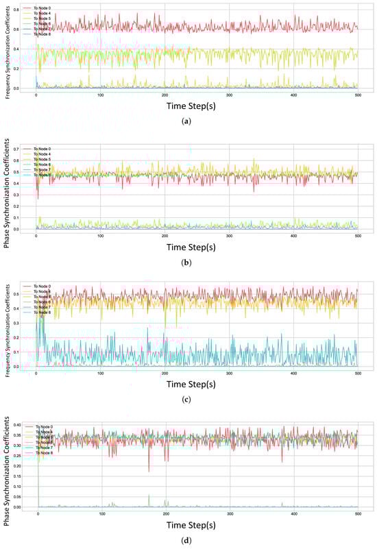
Figure 13. Real-time weight values output by the algorithm for Node 3. (a) The frequency weights at episode 100. (b) The frequency weights at episode 200. (c) The phase weights at episode 100. (d) The phase weights at episode 200.

As shown in Figure 14, we compare the system’s synchronization accuracy at the 100th episode (before the abrupt change) and at the 200th episode (100 episodes after the change). Before the change, after excluding anomalous nodes, the architecture had achieved a frequency synchronization accuracy of approximately $4\times {10}^{-10}$ and a phase synchronization accuracy of $1\times {10}^{-9}$ s. After experiencing the environmental change and completing its policy self-adaptation, the architecture’s synchronization performance dynamically adjusted to the new clock configuration, ultimately reaching a frequency accuracy of $2\times {10}^{-10}$ and a phase accuracy of $5\times {10}^{-10}$ s.

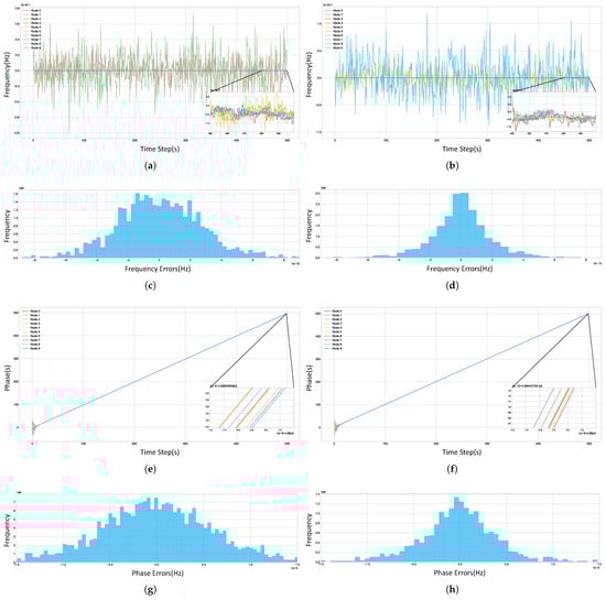
Figure 14. Time synchronization performance of the algorithm. (a) Frequency synchronization at episode 100; (b) at episode 200. (c) Histogram of node frequency differences vs. system average (last 300 time steps, episode 100, excluding anomalous nodes); (d) at episode 200. (e) Phase synchronization at episode 100; (f) at episode 200. (g) Histogram of node phase differences vs. system average (last 300 time steps, episode 100, excluding anomalous nodes); (h) at episode 200.

The experimental results demonstrate that the DDPG agent does not learn a fixed, static policy. Instead, it is capable of continuously evaluating the state of its neighbors and dynamically adjusting its “attention” allocation, thereby maintaining the optimality of its decisions and the robustness of the architecture in a non-stationary environment.

3.3. DSTS Experiment Results

In this section, we conduct an overall performance evaluation of the complete DSTS architecture and compare it against a widely used baseline method to verify its superiority in addressing clock heterogeneity and communication uncertainty. The experimental data was generated by accumulating the clock frequency and phase data from Figure 1 timestamps ($t_1,t_2,t_3,t_4,t_5,t_6$), as described in [17]. The fully trained DDPG model from Section 3.2.1 was employed as the decision-making back end for the DSTS architecture. The network topology remains consistent with Section 3.2, corresponding to the 10-node heterogeneous network shown in Figure 8.

To quantify the performance improvement of the DSTS architecture, we selected the widely applied average-consensus algorithm (AC) [11,13] as a baseline for comparison. This baseline method adheres to traditional distributed synchronization logic: each node acquires the frequency differences and corrected phase differences from all its neighbors and then uses their mean value as its own clock compensation value. This baseline represents a non-adaptive, static synchronization strategy.

Regarding the performance of the Bayesian filtering, Figure 15 visually compares the Phases Difference data for the link between Node 6 and Node 8 under monitor occlusion, both before and after Bayesian filtering. In the plot, the Observed Phase Difference exhibits sharp fluctuations and a high degree of randomness. The Raw Phases Difference represents the true phase difference calculated from the timestamps, while the Filtered Phases Difference is the phase difference output by our filtering algorithm. It can be clearly seen that the filtered signal aligns more closely with the true value.

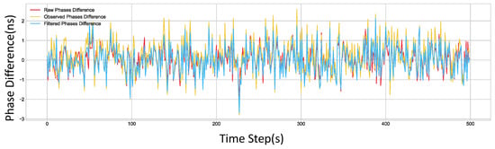
Figure 15. This figure shows the true phase offset, the phase offset calculated from observed values, and the phase offset calculated after filtering for the link between Node 6 and Node 8 at each time step.

Figure 16 displays the probability density distribution histograms of the error between the estimated phase difference and the true phase difference, both before and after filtering. The subplot corresponding to the error distribution of the observed phase difference shows a standard deviation of 0.718 ns. In contrast, after being processed by the filter, the standard deviation is reduced to 0.438 ns, indicating a closer alignment with the true phase difference.

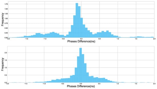
Figure 16. The top plot in this figure displays a histogram of the error between the phase offset calculated from observed values and the true phase offset. The bottom plot displays a histogram of the error between the phase offset calculated from filtered values and the true phase offset.

As illustrated in Figure 17, a comparison of the final synchronization performance between DSTS and the average-consensus algorithm shows that DSTS improves upon the baseline method in both accuracy and stability.

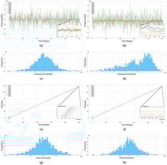
Figure 17. Time synchronization performance of the algorithm. (a) Frequency synchronization (DSTS); (b) frequency synchronization (AC). (c) Histogram of node frequency differences vs. system average (last 300 time steps, DSTS, excluding anomalous nodes); (d) the same as (c) (AC). (e) Phase synchronization (DSTS); (f) phase synchronization (AC). (g) Histogram of node phase differences vs. system average (last 300 time steps, DSTS, excluding anomalous nodes); (h) the same as (g) (AC).

The average-consensus algorithm, which performs non-differentiated averaging of information from all neighbors, allows significant errors from anomalous nodes to destabilize the entire network. This vulnerability ultimately limits the final precision the system can achieve. In contrast, the DDPG agent in the DSTS architecture leverages its adaptive “attention” mechanism to successfully identify and drastically reduce the weights of these unreliable information sources. This process effectively isolates their negative impact, enabling the remaining nodes in the network to converge to a consensus state that is far more precise and robust than that of the baseline method. Ultimately, the proposed DSTS architecture achieves a frequency synchronization accuracy of $4\times {10}^{-10}$ and a phase synchronization accuracy of $5\times {10}^{-10}$ s. The average-consensus algorithm, on the other hand, is unable to mitigate interference and only reaches a final accuracy of $2\times {10}^{-8}$ for frequency and $1\times {10}^{-7}$ s for phase—a level of precision far below the inherent stability of the high-quality clock sources present in the network.

To reflect the system’s overall time synchronization performance, we introduce the following formula, which we term SRAMSE:

$$SRAMSE=\sqrt{{\displaystyle \frac{1}{N}}\sum _{i=0}^N{\left(C_i-{\displaystyle \frac{1}{N-1}}\sum _{j=1}^N{C}_j\right)}^2}$$

(26)

where $C_i$ represents the clock reading of node i at the current time instant. The term $C_i-{\displaystyle \frac{1}{N-1}}{\sum }_{j=1}^N{C}_j$ quantifies the proximity of a node’s clock reading to the average reading of the other nodes in the network at that moment. A smaller SRAMSE value signifies that the clock readings among the nodes are closer, thus indicating higher synchronization accuracy.

The results are presented in Figure 18, which displays the SRAMSE evolution curves for both the DSTS and the average-consensus algorithm over the entire test process. While both algorithms converge to a stable synchronization state, there are significant differences in their final synchronization accuracy and stability.

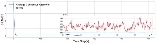
Figure 18. This figure shows the SRAMSE evolution curves for the DSTS and the Average Consensus algorithms.

During the last 200 time steps of the test, the DSTS method achieved an average SRAMSE of $4.628\times {10}^{-10}$ with a standard deviation of $2.015\times {10}^{-10}$. In comparison, the average-consensus algorithm yielded an average SRAMSE of $5.543\times {10}^{-8}$ and a variance of $2.467\times {10}^{-8}$.

4. Discussion

This study introduced the Distributed Sensor Time Synchronization architecture, a novel framework designed to provide robust, high-precision time synchronization for distributed sensor systems, particularly in the challenging, GNSS-denied environments where traditional methods falter. The experimental results robustly support our initial working hypotheses: first, that fusing Time-of-Flight and Channel Impulse Response data via Bayesian filtering can effectively mitigate non-linear communication errors, and second, that a Deep Deterministic Policy Gradient agent can intelligently manage clock heterogeneity and dynamic network conditions.

The performance of the DSTS architecture represents a significant advancement over existing methods. Traditional approaches often tackle communication errors and clock management as separate issues. For instance, while methods like those in [17,18,19] characterize NLOS errors and [27] uses a Deep Neural Network to identify NLOS conditions, our Bayesian filtering module provides a more dynamic solution by continuously estimating and compensating for ToF errors in real-time, reducing the standard deviation by over 41.2% in NLOS scenarios. This demonstrates a superior capability to handle the uncertainty inherent in wireless channels, a limitation noted in the comprehensive survey by [8]. Furthermore, conventional consensus algorithms, such as the average-consensus algorithm used as our baseline, assume node homogeneity and stable links. As our results show, this assumption breaks down in heterogeneous networks, where the AC algorithm’s performance is dragged down by the least stable nodes, achieving an accuracy of only $2\times {10}^{-8}$. In contrast, our DDPG-based approach, inspired by the attention mechanism, empowers each node to act as an autonomous agent. It learns to dynamically assign synchronization weights, effectively ignoring unstable neighbors or poor-quality links. This intelligent, adaptive weighting allowed DSTS to achieve a synchronization accuracy of $4\times {10}^{-10}$, better than the AC baseline.

However, we must acknowledge the limitations of our work. First, the architecture requires an initialization phase before deployment. Specifically, the Bayesian filtering module relies on statistical models pre-calibrated for specific operational scenarios, and the DDPG agents also require initial offline or online training to learn an effective synchronization policy. This may limit the system’s immediate applicability in sudden or entirely novel environments. Second, the computational demands of the DDPG agent could pose a challenge for deployment on highly resource-constrained edge devices common in remote sensing applications.

Regarding computational complexity and resource overhead, the Bayesian filtering module’s operational cost primarily depends on the chosen implementation for approximating the probability distribution. For the histogram filter, the complexity scales approximately as $O(G)$, where G is the number of grid points used to represent the state space. The DDPG agent’s complexity during the inference phase is dominated by the learning process through the Actor/Critic network in Figure 4. For the current network configuration, the Actor model’s file is approximately 80 kB, and the Critic model’s file size is approximately 150 kB. Its complexity can be characterized as $O({\sum }_{l=1}^L{N}_l{N}_{l-1})$, where L is the number of layers, and $N_l$ is the number of neurons in layer l ($N_0$ being the input dimension, $4\times d$). The input dimension depends on the number of neighbors d. Thus, the computational load increases with network density and the size of the neural network. Memory requirements are primarily for storing the network weights. While inference is less demanding than training, deployment on highly resource-constrained microcontrollers might necessitate optimizations. To provide an initial assessment of feasibility on embedded hardware, we conducted supplementary simulation training of the proposed DSTS architecture for a three-node fully connected network on an NVIDIA Jetson Orin NX platform. Each training episode took approximately 39 s. This result indicates that in future work, the DSTS architecture can be deployed on capable edge devices. One potential optimization strategy for the DDPG agent in dense networks is to initially screen neighbors based on channel state LOS/NLOS from Bayesian filter and clock stability (${\sigma }_j$). Neighbors identified as unreliable could have their initial synchronization weights effectively set to zero, reducing the effective number of neighbors (d) processed by the Actor network and thereby lowering the computational burden during runtime.

Regarding adaptability to other wireless systems beyond UWB, the DSTS framework’s core concepts—using Bayesian filtering for measurement refinement and reinforcement learning for adaptive weighting—are potentially generalizable. However, direct implementation requires careful consideration of the target technology’s capabilities. The Bayesian filter relies on ToF measurements and features indicative of channel conditions (like UWB CIR for LOS/NLOS differentiation) [5]. Technologies offering precise time-based ranging (e.g., Wi-Fi, 5G) might provide suitable ToF inputs, though extracting analogous channel features and recalibrating the filter’s statistical models would be necessary. Adapting the current filter design to primarily RSSI-based systems like LoRa would likely require substantial modifications. The DDPG agent requires inputs representing relative clock states, link quality, and neighbor stability. If such metrics can be derived from the target technology, the RL agent could potentially learn an effective weighting policy. Therefore, while the DSTS architecture offers potential adaptability, porting it to other systems like Wi-Fi, LoRa, or 5G would necessitate dedicated research and adaptation efforts.

5. Conclusions

This paper addressed the critical challenge of maintaining high-precision time synchronization among distributed sensor systems, particularly in the challenging, GNSS-denied environments. The architecture innovatively integrates Bayesian filtering with deep reinforcement learning to address the limitations of existing methods.The Bayesian filtering module effectively mitigates non-linear communication errors by fusing Time-of-Flight measurements with Channel Impulse Response features, successfully reducing the standard deviation of ToF measurements by over 41.2% in NLOS scenarios. Concurrently, the Deep Deterministic Policy Gradient algorithm empowers each network node to act as an intelligent agent. This agent autonomously learns to assign optimal synchronization weights based on local information, such as neighbor clock stability and link quality, thus adaptively amplifying the influence of reliable sources while mitigating the negative impact of unstable nodes and adverse channel conditions. Simulation experiments, based on a real-world UWB dataset, demonstrate the superior performance of the DSTS architecture. It achieved a final frequency and phase synchronization precision of $4\times {10}^{-10}$ and $5\times {10}^{-10}$ s, respectively. This represents a improvement in accuracy compared to the traditional average-consensus algorithm.

Future work will focus on several key areas to further enhance and validate the DSTS architecture. Firstly, physical implementation and testing on a real distributed sensor platform are crucial to definitively assess performance and robustness in diverse real-world challenging environments. Secondly, exploring the adaptation of the DSTS framework to other wireless technologies, such as Wi-Fi or 5G positioning signals, possibly requiring recalibration of the Bayesian models and tuning of the RL agent, represents a promising direction for broader applicability.

References

- Gao, D.; Liu, Y.; Hu, B.; Wang, L.; Chen, W.; Chen, Y.; He, T. Time Synchronization Based on Cross-Technology Communication for IoT Networks. IEEE Internet Things J. 2023, 10, 19753–19764. [Google Scholar] [CrossRef]
- Teng, F.; Yang, W.; Yan, J.; Ma, H.; Jiao, Y.; Gao, Z. A Parallel Solution of Timing Synchronization in High-Speed Remote Sensing Data Transmission. Remote Sens. 2023, 15, 3347. [Google Scholar] [CrossRef]
- Huang, S.; Cai, B.; Lu, D.; Zhao, Y.; Zhang, M.; Shang, L. Embedding Moving Baseline RTK for High-Precision Spatiotemporal Synchronization in Virtual Coupling Applications. Remote Sens. 2025, 17, 1238. [Google Scholar] [CrossRef]
- Li, X.; Huang, J.; Li, X.; Shen, Z.; Han, J.; Li, L.; Wang, B. Review of PPP–RTK: Achievements, challenges, and opportunities. Satell. Navig. 2022, 3, 28. [Google Scholar] [CrossRef]
- Dongare, A.; Lazik, P.; Rajagopal, N.; Rowe, A. Pulsar: A Wireless Propagation-Aware Clock Synchronization Platform. In Proceedings of the 2017 IEEE Real-Time and Embedded Technology and Applications Symposium (RTAS), Pittsburgh, PA, USA, 18–21 April 2017; pp. 283–292. [Google Scholar] [CrossRef]
- Xue, B.; Li, Z.; Lei, P.; Wang, Y.; Zou, X. Wicsync: A wireless multi-node clock synchronization solution based on optimized UWB two-way clock synchronization protocol. Measurement 2021, 183, 109760. [Google Scholar] [CrossRef]
- Aslam, M.; Liu, W.; Jiao, X.; Haxhibeqiri, J.; Miranda, G.; Hoebeke, J.; Marquez-Barja, J.; Moerman, I. Hardware Efficient Clock Synchronization Across Wi-Fi and Ethernet-Based Network Using PTP. IEEE Trans. Ind. Inform. 2022, 18, 3808–3819. [Google Scholar] [CrossRef]
- Puttnies, H.; Danielis, P.; Sharif, A.R.; Timmermann, D. Estimators for Time Synchronization—Survey, Analysis, and Outlook. IoT 2020, 1, 398–435. [Google Scholar] [CrossRef]
- Maróti, M.; Kusy, B.; Simon, G.; Lédeczi, A. The flooding time synchronization protocol. In Proceedings of the SenSys04: ACM Conference on Embedded Network Sensor Systems, Baltimore, MD, USA, 3–5 November 2004; Association for Computing Machinery: New York, NY, USA, 2004; pp. 39–49. [Google Scholar] [CrossRef]
- Elson, J.; Girod, L.; Estrin, D. Fine-grained network time synchronization using reference broadcasts. SIGOPS Oper. Syst. Rev. 2003, 36, 147–163. [Google Scholar] [CrossRef]
- Maggs, M.K.; O’Keefe, S.G.; Thiel, D.V. Consensus Clock Synchronization for Wireless Sensor Networks. IEEE Sens. J. 2012, 12, 2269–2277. [Google Scholar] [CrossRef]
- Gu, X.; Zheng, C.; Li, Z.; Zhou, G.; Zhou, H.; Zhao, L. Cooperative Localization for UAV Systems From the Perspective of Physical Clock Synchronization. IEEE J. Sel. Areas Commun. 2024, 42, 21–33. [Google Scholar] [CrossRef]
- Jin, X.; Ke, S.; An, J.; Wang, S.; Pan, G.; Niyato, D. A novel consensus-based distributed time synchronization algorithm in high-dynamic multi-UAV networks. IEEE Trans. Wirel. Commun. 2024, 23, 18916–18928. [Google Scholar] [CrossRef]
- Wang, T.; Xiong, H.; Ding, H.; Zheng, L. TDOA-based joint synchronization and localization algorithm for asynchronous wireless sensor networks. IEEE Trans. Commun. 2020, 68, 3107–3124. [Google Scholar] [CrossRef]
- Chen, C.; Li, L.; Peng, H.; Yang, Y.; Mi, L.; Zhao, H. A new fixed-time stability theorem and its application to the fixed-time synchronization of neural networks. Neural Netw. 2020, 123, 412–419. [Google Scholar] [CrossRef] [PubMed]
- Yu, K.; Wen, K.; Li, Y.; Zhang, S.; Zhang, K. A Novel NLOS Mitigation Algorithm for UWB Localization in Harsh Indoor Environments. IEEE Trans. Veh. Technol. 2019, 68, 686–699. [Google Scholar] [CrossRef]
- Peterseil, P.; Märzinger, D.; Etzlinger, B. UWB-Weak-NLOS-Structured-Dataset. Available online: https://github.com/ppeterseil/UWB-weak-NLOS-structured-dataset (accessed on 30 April 2025).
- Peterseil, P.; Etzlinger, B.; Märzinger, D.; Khanzadeh, R.; Springer, A. Data Trustworthiness for UWB Ranging in IoT. In Proceedings of the 2022 IEEE Globecom Workshops (GC Wkshps), Rio de Janeiro, Brazil, 4–8 December 2022; pp. 939–944. [Google Scholar] [CrossRef]
- Peterseil, P.; Märzinger, D.; Etzlinger, B.; Springer, A. Labeling for UWB Ranging in Weak NLOS Conditions. In Proceedings of the 2022 International Conference on Localization and GNSS (ICL-GNSS), Tampere, Finland, 7–9 June 2022; pp. 1–6. [Google Scholar] [CrossRef]
- Liu, P.; Zhang, S.; Zhou, Z.; Lv, L.; Huang, L.; Liu, J. Multiple satellite and ground clock sources-based high-precision time synchronization and lossless switching for distribution power system. IET Commun. 2023, 17, 2041–2052. [Google Scholar] [CrossRef]
- Yiğitler, H.; Badihi, B.; Jäntti, R. Overview of Time Synchronization for IoT Deployments: Clock Discipline Algorithms and Protocols. Sensors 2020, 20, 5928. [Google Scholar] [CrossRef]
- Maurizio Mongelli, S.S. A neural approach to synchronization in wireless networks with heterogeneous sources of noise. arXiv 2022, arXiv:2212.03327. [Google Scholar] [CrossRef]
- Lillicrap, T.P.; Hunt, J.J.; Pritzel, A.; Heess, N.; Erez, T.; Tassa, Y.; Silver, D.; Wierstra, D. Continuous control with deep reinforcement learning. arXiv 2015, arXiv:1509.02971. [Google Scholar] [CrossRef]
- Al-Okby, M.F.R.; Junginger, S.; Roddelkopf, T.; Thurow, K. UWB-Based Real-Time Indoor Positioning Systems: A Comprehensive Review. Appl. Sci. 2024, 14, 11005. [Google Scholar] [CrossRef]
- Wu, Y.; Yang, B.; Shenghong, X.; Maolei, W. Atomic Clock Models and Frequency Stability Analyses. Geomat. Inf. Sci. Wuhan Univ. 2019, 44, 1226–1232. [Google Scholar] [CrossRef]
- Jaduszliwer, B.; Camparo, J. Past, present and future of atomic clocks for GNSS. GPS Solut. 2021, 25, 27. [Google Scholar] [CrossRef]
- Goodarzi, M.; Sark, V.; Maletic, N.; Terán, J.G.; Caire, G.; Grass, E. DNN-Assisted Particle-Based Bayesian Joint Synchronization and Localization. IEEE Trans. Commun. 2022, 70, 4837–4851. [Google Scholar] [CrossRef]
Disclaimer/Publisher’s Note: The statements, opinions and data contained in all publications are solely those of the individual author(s) and contributor(s) and not of MDPI and/or the editor(s). MDPI and/or the editor(s) disclaim responsibility for any injury to people or property resulting from any ideas, methods, instructions or products referred to in the content. |
© 2025 by the authors. Licensee MDPI, Basel, Switzerland. This article is an open access article distributed under the terms and conditions of the Creative Commons Attribution (CC BY) license (https://creativecommons.org/licenses/by/4.0/).