GLFFEN: A Global–Local Feature Fusion Enhancement Network for Hyperspectral Image Classification

Highlights

What are the main findings?

• We found that many hyperspectral classifiers underperform due to ineffective integration of global contextual relationships and local spatial–spectral features and proposed GLFFEN, a novel HSI classification network that integrates dynamic graph reasoning and a spectral-attention CNN for global–local feature fusion.
• We introduced a multi-feature adaptive fusion (MAF) module for semantically aligned integration of heterogeneous features.

What are the implications of the main finding?

• GLFFEN achieves new SOTA accuracy across three benchmarks with high computational efficiency.
• The proposed feature extraction scheme and fusion strategy offer a generalizable fusion framework suitable for multimodal remote sensing tasks.

Abstract

Effective feature extraction is a key issue in hyperspectral image (HSI) classification task. Recent works have studied hyperspectral classification models based on various deep architectures. However, the specific architecture cannot fully exploit the complementary diversity of global and local features in HSIs, resulting in suboptimal results. To address these issues, we fully utilize the advantages of GNN and CNN in global and local feature extraction and design a new end-to-end global–local feature fusion enhancement network (GLFFEN). Specifically, we first construct a GNN with dynamically weighted neighbor contributions using superpixel-segmented patches as nodes, named the Graph Attention (GA) branch. Additionally, we design a spatial–spectral feature attention module (SSFAM) to enhance the ability of the CNN to extract spatial and spectral features in local neighborhoods, termed the spatial–spectral feature attention (SSFA) branch. Moreover, a multi-feature adaptive fusion (MAF) module is proposed to solve the problem of weight distribution during global–local feature fusion. Experiments on three well-known HSI datasets have shown that our GLFFEN surpasses state-of-the-art (SOTA) methods on three widely used metrics.

1. Introduction

The hundreds of continuous bands in hyperspectral images (HSIs) contain abundant spatial and spectral information [1,2]. In hyperspectral images, each pixel can be regarded as a high-dimensional vector, whose entries correspond to the spectral reflectance at specific wavelengths [3,4,5,6]. Hyperspectral images have the advantage of distinguishing subtle spectral differences and have been widely applied in many fields [7], such as environmental monitoring [8], precision agriculture [9], mineral exploration, and military recognition [10,11].

Hyperspectral images (HSIs) contain hundreds of contiguous spectral bands. While this high-dimensional information provides a basis for classification, it also introduces information redundancy and the Hughes phenomenon. Furthermore, due to their low spatial resolution, HSIs are prone to mixed-pixel effects, making classification based solely on spectral information prone to significant errors. Therefore, effective feature extraction is of great research significance in the field of HSI classification.

Early studies on HSI classification primarily relied on machine learning (ML) methods, including Random Forest [12], K-Nearest Neighbors (KNN) [13], Markov Random Fields [14], Gaussian Processes [15], and Support Vector Machines [16]. However, these methods often ignore spatial–contextual information, are sensitive to noise and outliers, and lack the capacity to capture deep semantic features.

The HSI classification model based on deep learning (DL) has become a cutting-edge research issue in recent years [17], and many network architectures have been applied in this field, including autoencoders (AEs) [18,19], recurrent neural networks (RNNs) [20], graph neural networks (GNNs) [21,22], Transformers [23], and Mamba [24,25]. Compared to machine learning, deep learning enables automatic high-dimensional feature extraction and supports end-to-end classification. The convolutional neural network (CNN), as a valuable paradigm, is widely applied in HSI classification tasks. A 1D-CNN [26] classifies HSIs spectrally using a five-layer convolutional structure, but overlook spatial relationships. A 2D-CNN incorporates neighboring pixel information to improve classification. Since HSI is intrinsically three-dimensional, Hamida et al. introduced a 3D-CNN [27] to simultaneously extract spectral and spatial features.

As researchers found that CNN could not adapt to the high dimensionality of hyperspectral images, Zhu et al. [28] proposed RSSAN with dual attention mechanism to suppress irrelevant spectral bands. However, RSSAN is constrained by its CNN-based structure and is prone to ignoring global information. In addition, Mamba [24,25] and Transformer [29,30] capture global features by establishing long-range dependencies in the spectrum sequence, but face challenges, including high computational resource demands and local information loss. Interestingly, SSGRAM [31] proposes a GNN paradigm that not only processes data directly within a local window, but also increases the computational burden. To reduce the computational burden, Wang et al. [32] designed a capsule attention network (CAN), combining activity vectors and attention mechanisms to improve the HSI classification. Notably, most existing HSI classification methods rely on the single backbone network, which fails to simultaneously capture both global and local features. Consequently, dual-backbone architectures with appropriate fusion strategies present significant research value for effectively integrating global and local representations.

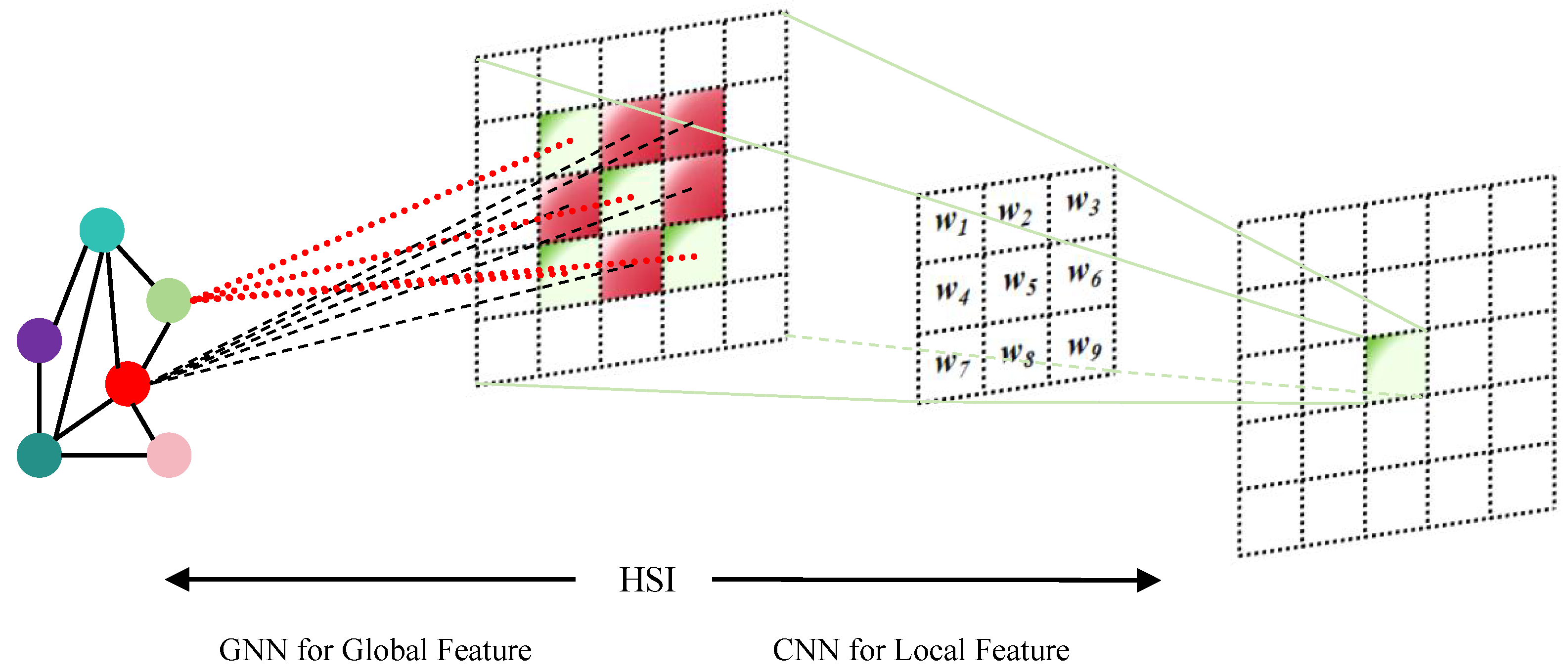
As shown in Figure 1, CNN-based feature extractors, constrained by their limited kernel sizes, primarily focus on local neighboring pixel features [33]. Consequently, while CNN demonstrates strong local feature extraction capabilities, its capabilities in capturing global representations are limited [34]. In contrast, GNN focuses on modeling correlations among pixels or patches across the global scope [35,36]. They classify pixels or patches based on these correlations to construct a graph [37]. With a global receptive field that transcends spatial constraints, GNNs excel at capturing long-range pixel dependencies but exhibit limited attention to local fine-grained features [38,39]. Thus, combining both backbone networks provides an effective solution for multi-scale feature extraction. The current mainstream GNN and CNN fusion methods significantly optimize classification accuracy compared to single backbone networks. However, the improvement brought by simple fusion strategies often leads to suboptimal results and heavy computational burdens. Thus, developing an effective global–local feature fusion module specifically for HSI data represents a viable approach to enhance classification accuracy [32]. To mitigate the limitations of fusion architectures, we propose a feature fusion enhancement network termed GLFFEN.

The main contributions of this research are as follows:

• We propose a global–local feature fusion enhancement network (GLFFEN) based on the combination of GNN and CNN. To reduce GNN’s computational load, we use the patches of superpixel segmentation (SLIC) as nodes to construct the graph, and use the multi-head attention-enhanced GNN contributed by dynamic weighted neighbors to construct the graph attention (GA) branch.
• We design a CNN-based spatial–spectral feature attention module (SSFAM) to extract local spatial–spectral features.
• In order to solve the problems of scale misalignment and information redundancy interference during feature fusion, we propose a multi-feature adaptive fusion (MAF) module to effectively integrate global and local representations.

Comparative experiments have shown that our method is superior to existing methods on three well-known datasets, and ablation experiments have been conducted to verify the effectiveness of the proposed GLFFEN.

2. Related Work

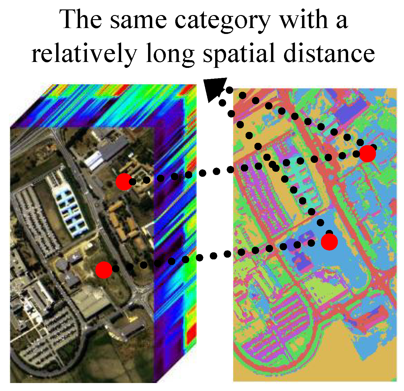
As shown in Figure 2, the spatially heterogeneous distribution of land-cover categories in HSIs poses challenges for CNN, as their regular grid-based feature extraction struggles to generalize across all image regions. In contrast, GNN overcomes this limitation by representing the image as a graph that transcends Euclidean distance constraints. They establish connections based directly on spectral similarity, thereby effectively aggregating spatially dispersed pixels belonging to the same category. Conversely, the detailed spatial patterns captured by CNN within local neighborhoods serve as robust features for initializing GNN nodes, while compensating for potential local detail loss caused by the topology-driven relational reasoning in GNNs. This complementary interaction enables the model to simultaneously perceive local details and establish global contextual relationships, thereby achieving robust classification of complex land-cover structures. By synergistically combining these architectures, the hybrid model can simultaneously leverage the CNN’s power in fine-grained feature extraction and the GNN’s ability to encode global semantic correlations, leading to enhanced representational capacity and improved classification accuracy, particularly in complex scenes with high inter-class variability.

2.1. Limitations of CNN for HSI Classification

CNN processes data at the pixel level and constructs non-linear mappings through the sequential stacking of convolutional operations, thereby progressively extracting high-level semantic features. If the cube of HSI is $X\in {\mathbb{R}}^{H\times W\times C}$, the dot product between each convolution computational input of the $\mathbf{l}$-th layer and the weight matrix $W\in {\mathbb{R}}^{H\times W\times C}$ is

$$\begin{array}{cc}\hfill f_{i,j,t}^{\left(l\right)}& ={\left({\mathbf{X}}^{\left(l\right)}\ast {\mathbf{W}}^{\left(l\right)}\right)}_{i,j,t}\hfill \\ \hfill & =\sum _{\widehat{i}=0}^{k-1}\sum _{\widehat{j}=0}^{k-1}\sum _{\widehat{t}=0}^{q-1}{x}_{(i·s+\widehat{i}),(j·s+\widehat{j}),(t·s+\widehat{t})}^{\left(l\right)}·w_{\widehat{i},\widehat{j},\widehat{t}}^{\left(l\right)}+b^{\left(l\right)}\hfill \end{array}$$

(1)

where $k\times k\times q$ denotes the kernel size, and s denotes the stride. $x_{\widehat{i},\widehat{j},\widehat{t}}^{\left(l\right)}$ and $w_{\widehat{i},\widehat{j},\widehat{t}}^{\left(l\right)}$ denote the input data and the weight of element $(\widehat{i},\widehat{j},\widehat{t})$. $f_{\widehat{i},\widehat{j},\widehat{t}}^{\left(l\right)}$ is the corresponding output after convolution. $b^{\left(l\right)}$ is the bias. Therefore, the obtained $F^{\left(l\right)}$ will be an array of scalar values. When processing hyperspectral images (HSI), the core convolutional operator of a CNN is intrinsically confined, by mathematical definition, to a local neighborhood of size $k\times k\times q$. To expand the receptive field, CNNs must rely on stacking convolutional layers and pooling operations. However, this leads to severe dilution of information between distant pixels through multiple nonlinear transformations, while downsampling via pooling sacrifices precise spatial structural information. Consequently, although the inductive bias of CNNs is beneficial for extracting local-hierarchical features, it fundamentally impedes the capture of global context.

In convolutional neural networks, both the size of the convolution kernel and the stride length are critical hyperparameters. The kernel essentially extracts statistical features from local image regions, which can be regarded as an approximate modeling of reflective properties within uniformly distributed pixel areas. The stride controls the interval at which the kernel moves across the input data. Fundamentally, convolution is an operation that numerically encodes local regions, enabling deeper architectures to capture higher-level semantic features through larger receptive fields [40]. However, constrained by its scalar-based representation, CNNs often require deep architectures stacked with multiple convolutional and nonlinear activation layers to achieve satisfactory performance. This approach not only increases model complexity but also introduces challenges to feature propagation across distant layers. Although classical models such as ResNet and DenseNet have partially alleviated gradient flow issues through identity mappings or dense connections, their substantial computational demands hinder deployment in resource-constrained scenarios. Particularly in hyperspectral image classification tasks, the limited representational capacity of scalar features becomes a notable performance bottleneck.

2.2. Limitations of GNN for HSI Classification

Graph Neural Network (GNN) models hyperspectral images (HSIs) as undirected graphs $\mathcal{G}=(\mathcal{V},\mathcal{E},\mathbf{A})$ to capture contextual relationships between land-cover categories. While GNN demonstrates considerable potential for HSI classification, it faces several inherent limitations that restrict its robustness and efficiency in practical applications.

The core operation in GNN involves iterative feature propagation through layer-wise updates. A standard Graph Neural Network (GNN) employs the propagation rule:

$${\mathbf{H}}^{(l+1)}=\sigma \left({\tilde{\mathbf{D}}}^{-{\displaystyle \frac{1}{2}}}\tilde{\mathbf{A}}{\tilde{\mathbf{D}}}^{-{\displaystyle \frac{1}{2}}}{\mathbf{H}}^{\left(l\right)}{\mathbf{W}}^{\left(l\right)}\right)$$

where $\tilde{\mathbf{A}}=\mathbf{A}+\mathbf{I}$ is the adjacency matrix with self-loops, $\tilde{\mathbf{D}}$ is the corresponding degree matrix, ${\mathbf{H}}^{\left(l\right)}$ contains node features at layer l, ${\mathbf{W}}^{\left(l\right)}$ denotes learnable weights, and $\sigma (·)$ is a nonlinear activation.

A pivotal challenge arises from the sensitive and often subjective graph construction process, which critically influences model performance yet heavily relies on heuristic hyperparameter selection. Furthermore, repeated application of the propagation rule leads to over-smoothing [41], where node features become increasingly similar through successive multiplications with the normalized adjacency matrix. This spectral smoothing effect disproportionately amplifies influences from distant nodes while diluting local detail, undermining the model’s capacity to capture fine-grained spatial structures in HSIs.

Additional limitations include substantial computational and memory overhead when scaling to typical hyperspectral data sizes [42], difficulties in modeling spectral–spatial heterogeneity, and heightened risk of overfitting under limited labeled samples. These issues collectively motivate research into more adaptive and scalable graph-based learning frameworks for HSI classification.

2.3. CNN-GNN Combined Models

TBDGCN [43] alleviates over-smoothing in GNNs through the incorporation of DropEdge and residual connections, and combines superpixel-level and pixel-level features. However, it suffers from high computational complexity, and its performance is strongly influenced by the quality of superpixel segmentation. WFCG [44] performs weighted integration of features from superpixel-based GAT and pixel-based CNN to explore high-dimensional characteristics. Yet, its fusion mechanism is relatively elementary and may fall short of facilitating deep interaction between heterogeneous features. MIAF-Net [45] employs an interactive attention mechanism to enhance mutual supplementation between local CNN features and global GCN topology, along with a hierarchical attention fusion module. Nonetheless, the model’s structural complexity results in elevated training difficulty and computational expense. Liu et al. [46] extracted features through multi-scale attentional graph convolution and a complementary dual convolutional attention network and introduced an attentional fusion pooling mechanism, yet this approach also faces challenges related to model complexity and computational overhead. NAGIN [37] enhances graph representation flexibility through adaptive neighborhood modeling, thereby boosting classification performance in complex scenarios. However, it maintains a pronounced sensitivity to hyperparameter configurations.

In contrast to the aforementioned methods, the proposed GLFFEN framework is designed to holistically address several recurring limitations in existing CNN-GNN fusion paradigms. Current approaches often face a critical trade-off: while methods relying on superpixels (e.g., TBDGCN) or adaptive graph structures (e.g., NAGIN) enhance modeling flexibility, they inherently suffer from sensitivity to segmentation quality or hyperparameter settings, compromising robustness. Furthermore, many fusion strategies, ranging from elementary weighted averaging (e.g., WFCG) to highly complex interactive attention modules (e.g., MIAF-Net), either fail to facilitate deep, hierarchical feature interactions or incur prohibitive computational costs. Motivated by these identified gaps, GLFFEN introduces a streamlined yet powerful architecture centered on a novel Multi-feature Adaptive Fusion (MAF) module. This design eliminates the dependency on explicit, high-quality superpixels and avoids intricate multi-stage feature extraction, enabling robust and efficient integration of heterogeneous spatial–spectral features. Consequently, GLFFEN establishes a superior balance between model performance, computational efficiency, and operational stability, presenting a cohesive solution that advances beyond the current state-of-the-art.

3. Materials and Methods

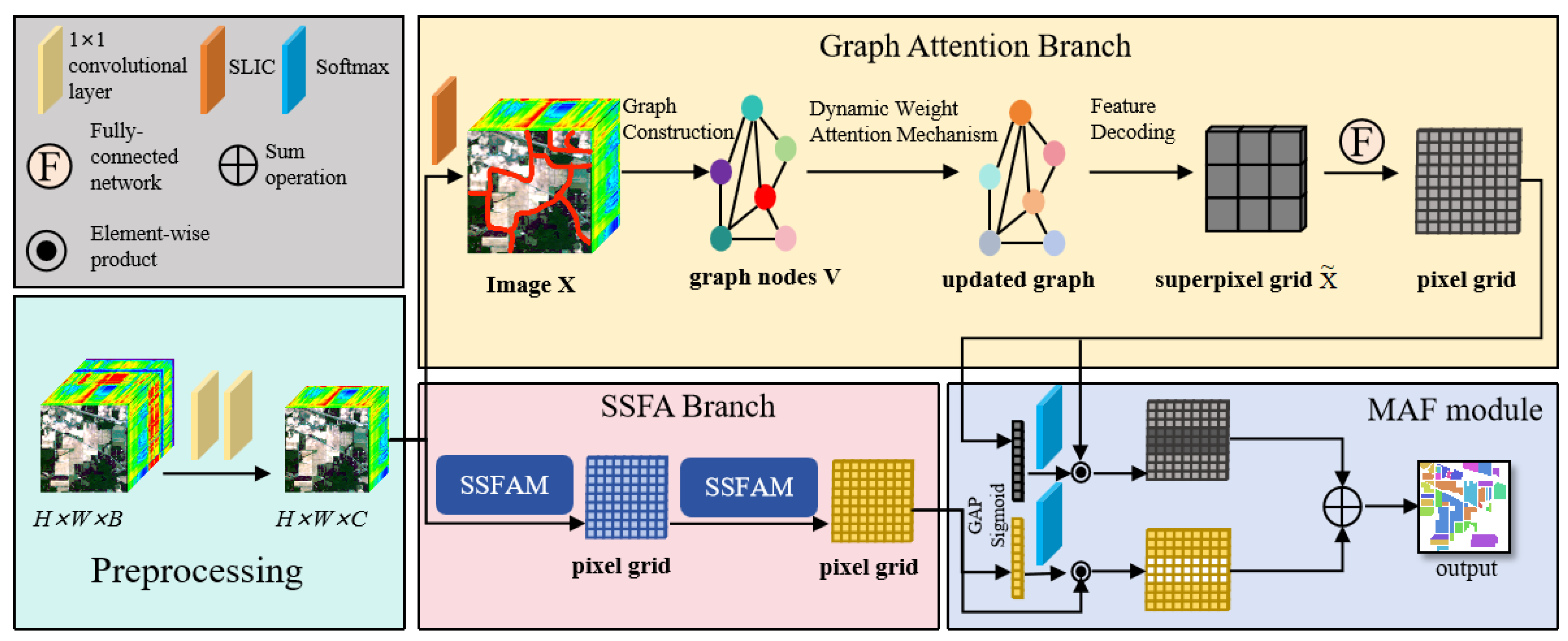
As shown in Figure 3, the GLFFEN framework pipeline consists of four key components: (1) preprocessing for spectral dimension reduction, (2) the GA branch for global feature extraction, (3) the SSFA branch for local feature extraction, and (4) the MAF module for global–local feature fusion.

We denote HSI as $X\in {\mathbb{R}}^{H\times W\times B}$. H, W, and B are denoted as the height, width, and the number of bands. We use two $1\times 1$ convolutional layers as the preprocessing step. The layers are used as cross-channel information exchange to remove useless spectral dimensions to strengthen discrimination ability and remove computational cost.

3.1. Graph Attention Branch

The GA branch is used to extract global features, mainly including four steps: Superpixel-based Graph Representation, Graph Construction, Dynamic Weight Attention Mechanism, and Feature Decoding.

3.1.1. Superpixel-Based Graph Representation

As shown in Figure 4, we adopt the Simple Linear Iterative Cluster (SLIC) superpixel algorithm [47] to aggregate adjacent pixels into homogeneous regions, thereby reducing computational complexity and enhancing structural coherence in subsequent graph construction. The algorithm operates in the CIELab color space augmented with spatial coordinates, forming extended feature vectors $(l,a,b,x,y)$ for each pixel. Initially, k cluster centers are sampled on a regular grid with interval $S=\sqrt{N/k}$, where N denotes the total number of pixels in the image. Each cluster center is subsequently optimized through iterative k-means clustering within a localized region of size $2S\times 2S$, minimizing a combined distance metric that balances color proximity and spatial adjacency. This process results in a partition of the image into compact, perceptually consistent superpixels, which serve as the foundational nodes of the graph $\mathcal{G}=(\mathcal{V},\mathcal{E},\mathbf{A})$ in our graph neural network architecture.

3.1.2. Graph Construction

The superpixel–pixel relationship is encoded in a binary association matrix $\mathbf{O}\in {(0,1)}^{N\times k}$, where ${\mathbf{O}}_{i,j}=1$ indicates pixel i belongs to superpixel j. The image $\mathbf{X}$ is transformed into graph nodes $\mathbf{V}$ via

$$\mathbf{V}={\tilde{\mathbf{O}}}^T\mathrm{Flatten}\left(\mathbf{X}\right),$$

(2)

where $\tilde{\mathbf{O}}$ is the column-normalized version of $\mathbf{O}$. Spatial adjacency defines the graph edges $\mathbf{E}$.

3.1.3. Dynamic Weight Attention Mechanism

To enhance traditional GNNs with adaptive neighbor weighting, we employ a multi-head attention mechanism that dynamically computes the importance of neighboring nodes. The feature transformation for each node i is given by the following equation:

$${\mathbf{h}}_i^{\prime }=\mathbf{W}{\mathbf{h}}_i$$

where $\mathbf{W}\in {\mathbb{R}}^{F\times F^{\prime }}$ is a shared weight matrix.

The attention mechanism computes normalized attention coefficients ${\alpha }_{ij}$ between connected nodes $(i,j)$ using the following equation:

$${\alpha }_{ij}={\displaystyle \frac{exp\left(\mathrm{LeakyReLU}\left({\mathbf{a}}^T[\mathbf{W}{\mathbf{h}}_i\parallel \mathbf{W}{\mathbf{h}}_j]\right)\right)}{{\sum }_{k\in {\mathcal{N}}_i}exp\left(\mathrm{LeakyReLU}\left({\mathbf{a}}^T[\mathbf{W}{\mathbf{h}}_i\parallel \mathbf{W}{\mathbf{h}}_k]\right)\right)}}$$

where $\mathbf{a}\in {\mathbb{R}}^{2F^{\prime }}$ is a learnable attention vector, and ${\mathcal{N}}_i$ denotes the neighborhood of node i.

Multi-head aggregation combines K independent attention heads:

$${\mathbf{h}}_i^{″}{=\parallel }_{k=1}^K\sigma \left(\sum _{j\in {\mathcal{N}}_i}{\alpha }_{ij}^k{\mathbf{W}}^k{\mathbf{h}}_j\right)$$

3.1.4. Feature Decoding

The graph representation is projected back to pixel space via

$$\tilde{\mathbf{X}}=\mathrm{Reshape}\left(\mathbf{O}\mathbf{V}\right),$$

(3)

where $\tilde{\mathbf{X}}\in {\mathbb{R}}^{H\times W\times C}$ represents the pixel-level feature mapping reconstructed from superpixel-level features, and $\mathbf{O}\mathbf{V}$ maps the node features back to the grid format.

For the output $\tilde{\mathbf{X}}$, it needs to be fed into a fully connected layer and projected into the same space as the output of the SSFA branch. This operation can place the outputs of the two branches in the same feature space to prepare for the MAF Module.

3.2. Spatial–Spectral Feature Attention Branch

The Spatial–Spectral Feature Attention Module (SSFAM) forms the core of our SSFA branch, with two SSFAMs arranged sequentially. As illustrated in Figure 5, each SSFAM comprises two principal components: the Spatial Feature Attention (SpaFA) block and the Spectral Feature Attention (SpeFA) block. These blocks are designed as efficient variants of the self-attention mechanism [48], leveraging global context modeling to enhance feature representations in their respective dimensions.

The proposed SSFAM differentiates itself from existing joint spatial–spectral attention mechanisms [49,50] through its sequential-decoupled architecture. While joint attention attempts to model interactions within a unified high-dimensional tensor—often incurring significant computational overhead and potential feature interference—the SSFAM processes spatial and spectral attentions separately. This design ensures a more efficient and hierarchical feature refinement: the SpaFA first establishes global contextual relationships across the image, upon which the SpeFA performs channel-wise recalibration. This sequential, decoupled approach mitigates the optimization difficulties of entangled feature spaces and yields a more computationally efficient and interpretable model compared to its joint counterparts.

3.2.1. SpaFA Block

The SpaFA block operates as a spatial self-attention mechanism that captures long-range dependencies across spatial positions [51]. SpaFA constructs a global spatial attention map by calculating the correlation between any two positions in the feature map. Its core mechanism lies in enabling features to interact in the spatial dimension through matrix transpose and multiplication, thereby encoding the spatial context information at a distance to each pixel position, thus overcoming the local receptive field limitation of traditional convolution and enhancing the model’s overall perception of the spatial layout of ground objects. Formally, given an input feature map $\mathbf{X}\in {\mathbb{R}}^{H\times W\times C}$, we generate query, key, and value projections through linear transformations:

$${\mathbf{Q}}_s={\mathbf{W}}_q\mathbf{X},{\mathbf{K}}_s={\mathbf{W}}_k\mathbf{X},{\mathbf{V}}_s={\mathbf{W}}_v\mathbf{X},$$

(4)

where ${\mathbf{W}}_q,{\mathbf{W}}_k,{\mathbf{W}}_v\in {\mathbb{R}}^{C\times C}$ are learnable weight matrices. The spatial attention map is computed via scaled dot-product attention:

$${\mathbf{M}}_s=\mathrm{softmax}\left({\displaystyle \frac{{\mathbf{Q}}_s{\mathbf{K}}_s^T}{\sqrt{d_k}}}\right),$$

(5)

where $d_k$ represents the dimension of the key vectors. The enhanced spatial features are obtained through the following equation:

$${\mathbf{X}}^{\prime }=\gamma {\mathbf{M}}_s{\mathbf{V}}_s+\mathbf{X},$$

(6)

where $\gamma$ is a learnable scaling parameter. This formulation enables global contextual modeling while preserving the original feature details through residual connection.

3.2.2. SpeFA Block

The SpeFA block functions as a channel self-attention mechanism that models interdependencies between spectral bands [51]. SpeFA focuses on feature recalibration in the channel dimension, explicitly modeling channel dependencies by constructing a covariance matrix between channels. The principle is to have the features of each channel accept the global information of all channels and undergo nonlinear transformation, thereby adaptively emphasizing spectral bands rich in discriminative information and suppressing redundant channels. Taking the spatially enhanced features ${\mathbf{X}}^{\prime }$ as input, we compute the channel attention map following the self-attention paradigm:

$${\mathbf{Q}}_c={\mathbf{X}}^{\prime }{\mathbf{W}}_q^{\prime },{\mathbf{K}}_c={\mathbf{X}}^{\prime }{\mathbf{W}}_k^{\prime },{\mathbf{V}}_c={\mathbf{X}}^{\prime }{\mathbf{W}}_v^{\prime },$$

(7)

where ${\mathbf{W}}_q^{\prime },{\mathbf{W}}_k^{\prime },{\mathbf{W}}_v^{\prime }\in {\mathbb{R}}^{C\times C}$ are learnable parameters. The channel attention is computed as follows:

$${\mathbf{M}}_c=\mathrm{softmax}\left({\displaystyle \frac{{\mathbf{Q}}_c{\mathbf{K}}_c^T}{\sqrt{d_k^{\prime }}}}\right),$$

(8)

with the final output obtained through

$${\mathbf{X}}^{″}=\beta {\mathbf{V}}_c{\mathbf{M}}_c^T+{\mathbf{X}}^{\prime },$$

(9)

where $\beta$ is a learnable parameter. This spectral attention mechanism adaptively emphasizes discriminative spectral bands while suppressing redundant information, completing the hierarchical feature refinement process.

3.3. Multi-Feature Adaptive Fusion Module

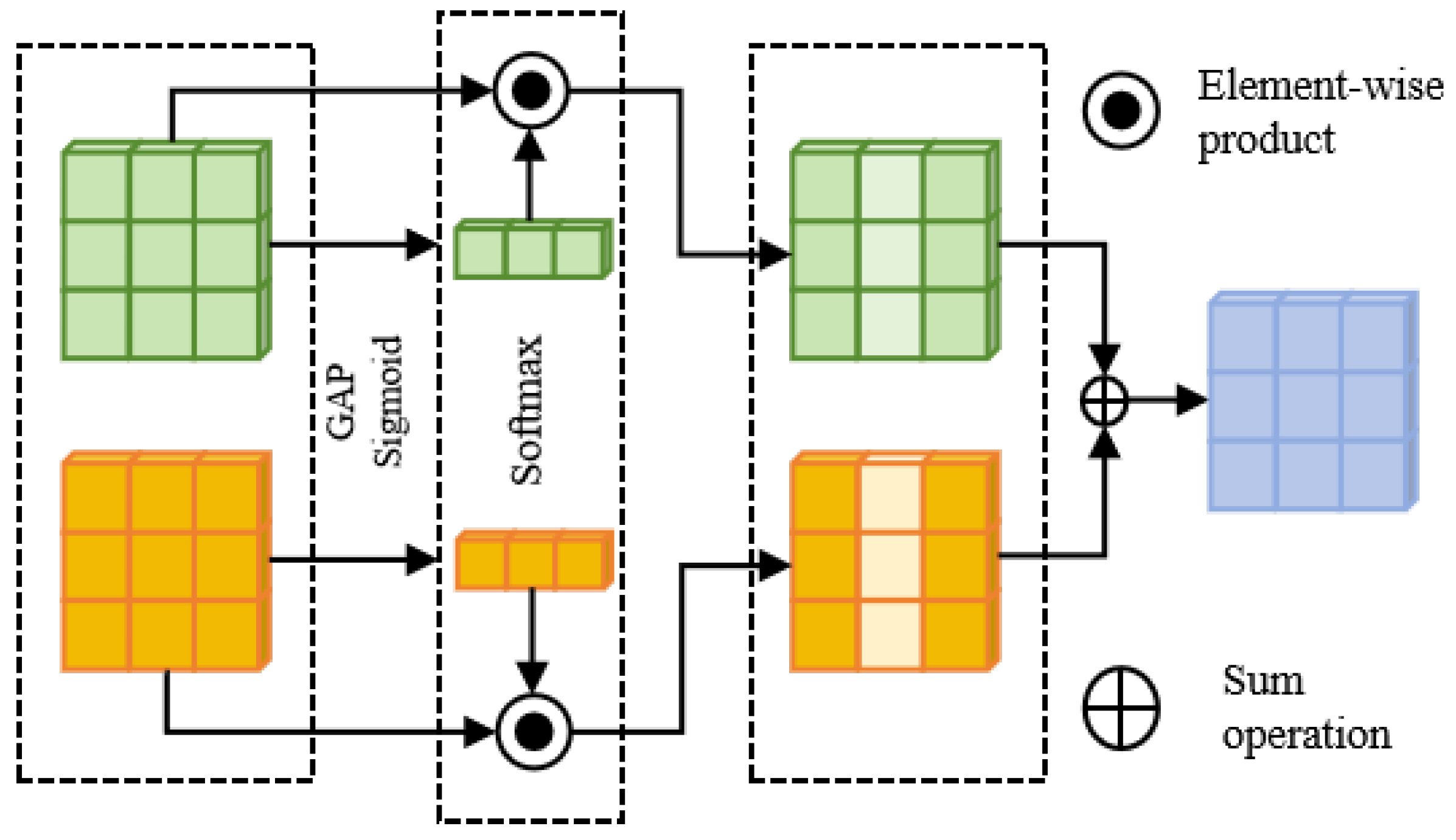
The proposed Multi-feature Adaptive Fusion (MAF) module addresses feature misalignment and shallow interaction in fusion through a dual-path architecture that explicitly processes macro-scale contextual patterns and micro-scale spatial details. The module employs a gated attention mechanism, implemented via a squeeze-and-excitation block, to generate dynamic channel-wise weights that resolve feature conflicts through non-linear recombination. This enables selective enhancement of complementary features while suppressing redundancies. Positioned after deep backbone networks, the module performs high-level aggregation of semantically rich features, preventing semantic dilution while maintaining discriminative power through coherent integration of multi-scale representations.

The network structure of the MAF module is shown in Figure 6. Given global and local features representations with the same shape: $[{\mathbf{F}}_0,{\mathbf{F}}_1\in {\mathbb{R}}^{C\times H\times W}]$. Firstly, the global feature representation is obtained through the global average pool (GAP) operation in the spatial dimension. Then, the correlation between channels is modeled by $\mathbf{1}\times \mathbf{1}\mathbf{Conv}$, and the channel descriptors are generated through the sigmoid activation function:

$$\begin{array}{cc}\hfill {\mathbf{F}}_0^{\prime }\in {\mathbb{R}}^{C\times 1\times 1}& =\mathbf{Sigmoid}\left(\mathbf{Conv}\left(\mathbf{GAP}\left({\mathbf{F}}_0\right)\right)\right),\hfill \\ \hfill {\mathbf{F}}_1^{\prime }\in {\mathbb{R}}^{C\times 1\times 1}& =\mathbf{Sigmoid}\left(\mathbf{Conv}\left(\mathbf{GAP}\left({\mathbf{F}}_1\right)\right)\right).\hfill \end{array}$$

(10)

Then, the global and local features are concatenated in the second dimension to obtain ${\mathbf{F}}^{″}\in {\mathbb{R}}^{C\times N\times 1}$, and the respective weights are obtained through the softmax function:

$${\mathbf{F}}^{\prime \prime }=\mathbf{Concat}({\mathbf{F}}_0^{\prime },{\mathbf{F}}_1^{\prime }),$$

(11)

$$\mathbf{W}\in {\mathbb{R}}^{C\times N\times 1}=\mathrm{softmax}\left({\mathbf{F}}^{″}\right).$$

(12)

Perform element-wise product on the generated weights with the corresponding inputs and add them together:

$$\mathbf{Y}=\mathbf{W}[:,0,:]\odot {\mathbf{F}}_0+\mathbf{W}[:,1,:]\odot {\mathbf{F}}_1,$$

(13)

where $\mathbf{Y}\in {\mathbb{R}}^{C\times H\times W}$ represents feature representation after fusion, ⊙ denotes element-wise product, and $\mathbf{W}[:,i,:]\in {\mathbb{R}}^{C\times 1\times 1}$.

3.4. Loss Function

The identity loss and reconstruction loss are used to train the proposed GLFFEN. The identity loss operates at the feature extraction level by imposing constraints on both the GA and SSFA branches to preserve the input’s spectral-spatial identity information. This mechanism effectively prevents critical discriminative features from being diminished during complex encoding-decoding transformations. The enforced identity consistency promotes tighter clustering of homogeneous samples and greater separation of heterogeneous samples in the feature space. Consequently, this enhancement in feature discriminability directly contributes to improved classification accuracy, with particularly notable gains observed in classifying minority categories and complex geographical boundaries.

$$\mathcal{L}=\alpha ·{\mathcal{L}}_{\mathrm{r}}+\beta ·{\mathcal{L}}_{\mathrm{i}},$$

(14)

where $\mathcal{L}$ denotes the overall loss, and ${\mathcal{L}}_{\mathrm{r}}$, and ${\mathcal{L}}_{\mathrm{i}}$ denote the reconstruction loss and the identity loss. $\alpha$ and $\beta$ are the weights of the loss.

3.4.1. Reconstruction Loss

Calculate the difference between the predicted value and the target value using the mean square error (MSE):

$${\mathcal{L}}_{\mathrm{r}}={\displaystyle \frac{1}{N}}\sum _{i=1}^N{(y_i-{\widehat{y}}_i)}^2,$$

(15)

where $y_i$ denotes the groud truth (GT) value, ${\widehat{y}}_i$ denotes the predicted value.

3.4.2. Identity Loss

Generate an output map through the pre-trained IdentityMLP, and then calculate the MSE between it and the input:

$${\mathcal{L}}_{\mathrm{i}}=\mathrm{IdentityMLP}\left(y\right),$$

(16)

where IdentityMLP is a pre-trained identity mapping model, with y as the input and the transformation result that maintains the structure unchanged as the output.

4. Experimental Results

Section 4.1 introduces the used hyperspectral datasets. Section 4.2 introduces implementation details. Section 4.3 shows the comparisons with SOTA methods.

4.1. Datasets Description

In the comparative experiment, we use three well-known datasets, namely Indian Pines (IP), University of Houston 2013 (UH2013), and Salinas University (SA).

The IP dataset was collected by the AVIRIS sensor from a scene in northwestern Indiana, USA, containing 145 × 145 pixels and 224 bands. After eliminating some interfering bands, there are still 200 bands remaining. This dataset has a total of 10,249 labeled pixels, which are divided into 16 feature categories. We select 435 samples as the training data and 9814 samples as the test data.The distribution of samples is summarized in

Table 1. Category information of IP dataset.

ClassID	Class Name	Training	Testing
1	Alfalfa	15	31
2	Corn-notill	30	1398
3	Corn-mintill	30	800
4	Corn	30	207
5	Grass-pasture	30	453
6	Grass-trees	30	700
7	Grass-pasture-mowed	15	13
8	Hay-windrowed	30	448
9	Oats	15	5
10	Soybeans-notill	30	942
11	Soybean-mintill	30	2425
12	Soybean-clean	30	563
13	Wheat	30	175
14	Woods	30	1235
15	Buildings-grass-trees-drivers	30	356
16	Stone-steel-towers	30	63
Total		435	9814

.

The UH2013 dataset measures 349 × 1905, has 144 effective bands, covers 15 types of land cover categories, and has a spatial resolution of 2.5 m. During this experiment, 450 samples are selected as training data, and 14,579 samples are used as test data. The distribution of samples is summarized in

Table 2. Category information of UH2013 dataset.

ClassID	Class Name	Training	Testing
1	Healthy grass	30	1221
2	Stressed grass	30	1224
3	Synthetic grass	30	667
4	Trees	30	1214
5	Soil	30	1212
6	Water	30	295
7	Residential	30	1238
8	Commercial	30	1214
9	Road	30	1222
10	Highway	30	1197
11	Railway	30	1205
12	Parking Lot 1	30	1203
13	Parking Lot 2	30	439
14	Tennis Court	30	398
15	Running Track	30	630
Total		450	14,579

.

The SA dataset was captured by the AVIRIS sensor over a scene in Salinas Valley, California. It consists of 512 × 217 pixels and 224 spectral bands. After removing noisy and water-absorption bands, 204 bands remain. The dataset contains 54,129 labeled pixels representing 16 distinct land-cover classes. In our experiments, 480 samples were used for training and 53,649 samples for testing. The distribution of samples is summarized in

Table 3. Category information of SA dataset.

ClassID	Class Name	Training	Testing
1	Brocoli_green_weeds_1	30	1979
2	Brocoli_green_weeds_2	30	3696
3	Fallow	30	1946
4	Fallow_rough_plow	30	1364
5	Fallow_smooth	30	2648
6	Stubble	30	3929
7	Celery	30	3549
8	Grapes_untrained	30	11,241
9	Soil_vineyard_develop	30	6173
10	Corn_senesced_green_weeds	30	3248
11	Lettuce_romaine_4wk	30	1038
12	Lettuce_romaine_5wk	30	1897
13	Lettuce_romaine_6wk	30	886
14	Lettuce_romaine_7wk	30	1040
15	Vinyard_untrained	30	7238
16	Vinyard_vertical_trellis	30	1777
Total		480	53,649

.

4.2. Implementation Details

All comparison methods are run on the NVIDIA RTX 4070 GPU using the PyTorch 1.12.1 framework and python3.8. Meanwhile, the Adam optimizer is used for training, with the learning rate set to $5\times {10}^{-4}$. Epoch is set at 300, and the batch size is 128.

4.3. Comparisons with SOTA Methods

In order to prove the effectiveness of the method we propose, we compare the proposed method with five advanced methods proposed in recent years: the Mamba-based method MMB [24], the Transformer-based method SF [29], the CNN-based method RSSAN [28], the GNN-based method SSGRAM [31], the Hybrid model methods AMGCFN [52] and NAGIN [37].

The classification effects of the comparative experiments are evaluated by average accuracy (AA), overall accuracy (OA), and Kappa coefficient. Additionally, we will also present the visual classification results.

4.3.1. Quantitative Analysis

Table 4. Quantitative comparison on IP dataset. Numbers in bold denote the best value in comparison to others.

Class	MMB	SF	RSSAN	SSGRAM	AMGCFN	NAGIN	OURS
1	56.14 ± 3.3	47.31 ± 13.5	31.18 ± 25.8	89.23 ± 3.1	100.0 ± 0.0	91.27 ± 0.7	94.25 ± 1.0
2	90.30 ± 0.5	50.74 ± 5.0	60.94 ± 13.5	95.63 ± 0.6	83.08 ± 10.1	90.32 ± 0.9	100.00 ± 0.0
3	91.45 ± 1.6	57.04 ± 6.7	64.75 ± 9.2	96.47 ± 0.0	88.87 ± 7.2	83.36 ± 0.8	98.33 ± 0.7
4	91.02 ± 0.9	84.06 ± 6.3	90.02 ± 4.9	88.69 ± 1.4	100.0 ± 0.0	96.94 ± 0.7	100.00 ± 0.0
5	91.02 ± 0.9	72.33 ± 6.6	83.81 ± 5.8	98.31 ± 0.9	95.12 ± 5.0	94.27 ± 0.7	100.00 ± 0.0
6	99.46 ± 0.6	82.29 ± 0.9	90.95 ± 2.9	100.0 ± 0.0	97.37 ± 1.3	97.21 ± 0.3	94.19 ± 1.2
7	98.63 ± 1.3	100.0 ± 0.0	100.0 ± 0.0	100.0 ± 0.0	100.0 ± 0.0	99.64 ± 0.2	100.00 ± 0.0
8	100.0 ± 0.0	96.35 ± 1.2	99.26 ± 0.5	100.0 ± 0.0	99.77 ± 0.1	100.0 ± 0.0	100.0 ± 0.0
9	100.0 ± 0.0	100.0 ± 0.0	100.0 ± 0.0	91.97 ± 1.1	100.0 ± 0.0	100.0 ± 0.0	99.60 ± 0.1
10	86.03 ± 2.0	71.09 ± 4.6	78.91 ± 8.6	83.21 ± 0.8	83.24 ± 6.5	100.0 ± 0.0	99.83 ± 0.1
11	93.67 ± 1.2	53.46 ± 9.3	56.78 ± 8.6	98.81 ± 0.2	90.03 ± 6.3	98.04 ± 0.6	99.26 ± 0.3
12	92.67 ± 1.3	43.64 ± 4.4	65.78 ± 4.3	91.42 ± 0.8	90.98 ± 5.1	96.54 ± 0.8	100.0 ± 0.0
13	96.67 ± 1.1	97.71 ± 1.6	98.48 ± 0.9	97.56 ± 0.1	99.61 ± 0.5	98.44 ± 0.9	97.38 ± 0.6
14	97.96 ± 0.9	76.60 ± 5.1	96.06 ± 0.4	100.0 ± 0.0	97.18 ± 0.4	99.83 ± 0.1	98.65 ± 0.5
15	94.32 ± 0.6	85.49 ± 3.3	79.78 ± 7.2	96.63 ± 0.4	97.18 ± 0.4	96.26 ± 0.3	100.0 ± 0.0
16	99.47 ± 0.7	98.94 ± 1.5	98.41 ± 1.3	86.63 ± 1.4	99.47 ± 0.7	100.0 ± 0.0	99.82 ± 0.0
OA (%)	92.76 ± 1.2	65.24 ± 2.0	73.78 ± 1.0	93.87 ±0.9	91.25 ± 4.8	95.14 ± 0.8	97.97 ± 0.7
AA (%)	92.34 ± 1.3	76.07 ± 0.9	80.94 ± 1.2	94.73 ±1.2	95.21 ± 5.4	96.73 ± 0.8	98.04 ± 0.4
Kappa	91.69 ± 1.4	61.06 ± 2.1	70.48 ± 0.9	92.09 ±1.0	90.03 ± 5.4	95.45 ± 0.6	97.38 ± 1.0

,

Table 5. Quantitative comparison on UH2013 dataset. Numbers in bold denote the best value in comparison to others.

Class	MMB	SF	RSSAN	SSGRAM	AMGCFN	NAGIN	OURS
1	93.61 ± 0.6	91.10 ± 3.8	90.72 ± 4.4	88.36 ± 0.4	86.09 ± 1.3	92.36 ± 0.7	95.17 ± 0.6
2	98.53 ± 0.4	93.19 ± 2.5	97.49 ± 1.5	88.68 ± 3.6	87.84 ± 9.2	96.63 ± 0.4	100.00 ± 0.0
3	94.15 ± 0.6	93.90 ± 4.6	99.15 ± 0.6	94.21 ± 0.7	97.35 ± 0.2	94.78 ± 0.8	96.74 ± 0.6
4	97.03 ± 0.1	88.44 ± 2.6	95.09 ± 3.4	84.63 ± 2.7	90.04 ± 1.9	95.31 ± 0.7	98.93 ± 0.3
5	94.58 ± 0.7	97.14 ± 0.6	94.39 ± 5.6	87.16 ± 1.4	99.42 ± 0.7	91.17 ± 0.9	99.84 ± 0.1
6	76.95 ± 3.1	88.36 ± 3.9	89.83 ± 5.5	93.84 ± 0.7	92.65 ± 0.6	66.72 ± 2.5	93.22 ± 0.8
7	95.10 ± 0.4	74.18 ± 1.9	84.41 ± 3.8	90.56 ± 2.1	92.16 ± 2.5	88.64 ± 0.8	97.33 ± 0.2
8	72.16 ± 2.8	76.44 ± 4.5	71.17 ± 4.9	92.47 ± 0.9	71.92 ± 3.5	97.62 ± 0.7	91.10 ± 0.4
9	91.57 ± 0.3	67.59 ± 3.7	83.42 ± 4.8	84.63 ± 2.7	76.28 ± 4.5	94.90 ± 0.5	93.96 ± 0.2
10	82.79 ± 2.3	78.75 ± 3.6	68.64 ± 10.9	85.06 ± 0.4	87.49 ± 4.8	92.27 ± 0.4	91.96 ± 0.4
11	89.79 ± 1.2	62.38 ± 6.0	66.25 ± 8.1	93.35 ± 0.7	88.98 ± 4.4	92.75 ± 0.2	97.14 ± 0.6
12	82.71 ± 4.2	74.40 ± 5.5	79.30 ± 5.3	88.16 ± 0.7	82.76 ± 12.0	96.84 ± 0.1	95.11 ± 0.4
13	66.97 ± 3.2	64.16 ± 5.6	92.71 ± 1.1	90.51 ± 0.4	88.61 ± 0.6	82.89 ± 0.7	82.19 ± 1.4
14	98.74 ± 0.4	88.86 ± 1.4	69.93 ± 1.6	98.36 ± 0.7	97.25 ± 0.7	94.31 ± 0.8	99.25 ± 0.3
15	99.84 ± 0.1	98.52 ± 0.9	93.02 ± 8.8	96.36 ± 0.8	98.72 ± 0.4	96.73 ± 1.0	100.0 ± 0.0
OA (%)	90.2 ± 0.6	81.68 ± 0.6	84.36 ± 3.0	93.74 ± 0.7	88.07 ± 2.0	91.36 ± 0.6	96.11 ± 0.3
AA (%)	89.33 ± 0.5	82.49 ± 0.1	85.03 ± 4.6	92.13 ± 0.7	89.58 ± 1.6	89.59 ± 0.8	95.23 ± 0.5
Kappa	89.39 ± 0.7	80.22 ± 0.7	83.08 ± 3.3	91.45 ± 0.9	87.09 ± 2.2	90.49 ± 0.7	95.66 ± 0.3

and

Table 6. Quantitative comparison on SA dataset. Numbers in bold denote the best value in comparison to others.

Class	MMB	SF	RSSAN	SSGRAM	AMGCFN	NAGIN	OURS
1	99.70 ± 0.2	94.74 ± 0.9	98.84 ± 0.2	99.34 ± 0.3	100.0 ± 0.0	99.84 ± 0.1	99.92 ± 0.0
2	99.89 ± 0.1	98.82 ± 0.4	99.50 ± 0.0	100.0 ± 0.0	99.72 ± 0.4	99.81 ± 0.0	100.00 ± 0.0
3	96.67 ± 0.6	92.17 ± 1.9	97.14 ± 1.8	100.0 ± 0.0	99.95 ± 0.1	99.84 ± 0.0	99.74 ± 0.1
4	96.87 ± 0.7	96.26 ± 0.9	99.49 ± 0.4	98.69 ± 0.3	98.53 ± 2.2	99.72 ± 0.0	99.77 ± 0.1
5	99.94 ± 0.0	89.41 ± 1.8	96.99 ± 1.2	97.87 ± 0.7	97.25 ± 0.7	99.62 ± 0.2	99.84 ± 0.1
6	99.93 ± 0.0	99.20 ± 0.7	99.02 ± 0.6	99.96 ± 0.0	99.59 ± 0.6	99.96 ± 0.0	100.00 ± 0.0
7	99.92 ± 0.0	97.91 ± 1.9	98.07 ± 1.6	99.80 ± 0.2	99.99 ± 0.0	99.97 ± 0.0	100.00 ± 0.0
8	88.38 ± 0.9	73.07 ± 1.1	71.60 ± 1.7	79.52 ± 6.7	83.51 ± 9.2	91.55 ± 0.4	94.35 ± 0.4
9	99.80 ± 0.2	93.77 ± 1.4	98.15 ± 0.9	99.90 ± 0.1	99.96 ± 0.0	99.62 ± 0.1	99.64 ± 0.1
10	95.78 ± 0.9	91.39 ± 1.8	92.03 ± 2.8	94.71 ± 2.0	99.61 ± 0.3	96.39 ± 0.7	99.93 ± 0.1
11	97.57 ± 0.3	92.36 ± 3.3	96.76 ± 1.8	98.74 ± 0.5	99.33 ± 0.5	99.27 ± 0.0	99.62 ± 0.2
12	99.83 ± 0.1	99.05 ± 0.5	99.37 ± 0.7	100.0 ± 0.0	99.91 ± 0.1	99.64 ± 0.1	96.44 ± 0.7
13	99.62 ± 0.2	99.40 ± 0.4	99.44 ± 0.6	96.77 ± 0.0	99.85 ± 0.1	99.88 ± 0.1	99.96 ± 0.0
14	98.68 ± 0.6	96.60 ± 0.9	95.54 ± 2.7	98.04 ± 0.7	99.23 ± 0.3	99.50 ± 0.2	93.53 ± 0.6
15	83.36 ± 0.7	81.58 ± 2.2	79.07 ± 3.1	84.93 ± 7.1	89.77 ± 10.3	90.03 ± 0.8	100.0 ± 0.0
16	98.76 ± 0.5	93.72 ± 2.0	95.72 ± 2.5	99.15 ± 0.4	99.90 ± 0.1	99.16 ± 0.3	99.83 ± 0.1
OA (%)	94.63 ± 0.5	88.80 ± 0.2	89.66 ± 0.76	92.58 ± 1.0	94.87 ± 1.0	95.82 ± 0.3	97.93 ± 0.1
AA (%)	95.77 ± 0.3	93.09 ± 0.1	94.79 ± 0.71	94.77 ± 0.4	97.10 ± 0.1	97.92 ± 0.3	99.17 ± 0.1
Kappa	96.45 ± 0.2	87.57 ± 0.2	88.53 ± 0.83	91.97 ± 1.1	89.98 ± 0.7	95.82 ± 0.4	97.88 ± 0.1

show the quantitative results of the IP, UH2013, and SA datasets. For the Mamba-based method, MMB performs well in the global classification distribution, but due to the loss of local details, its classification accuracy still lags behind GLFFEN and SSGRAM. The SF only focuses on the long-range relationships of spectral sequences; thus, a large number of errors occur in the classification results. For RSSAN, even though the combination of spatial–spectral features makes its classification effect better than SF, due to the low attention to global features, the performance is still poor, especially on the IP dataset. SSGRAM based on GNN uses graph attention map to enhance global feature extraction and has achieved an effect second only to GLFFEN in classification accuracy. Although the hybrid model AMGCFN has advantages compared with some single-backbone methods, its simple fusion strategy leads to a gap compared with MMB and SSGRAM. In comparison with AMGCFN, Nagin improves the fusion strategy by employing an adaptive neighborhood graph isomorphism network for feature extraction and relational reasoning. However, as Nagin places greater emphasis on abstract node relationships rather than preserving original spatial textures, substantial detailed information is lost. Nevertheless, it still achieves suboptimal performance on both the IP and SA datasets, demonstrating that a well-designed dual-backbone architecture can effectively enhance classification accuracy. The GLFFEN we proposed achieves the optimal results on both datasets. The results show that classification using global and local feature fusion can better fit the HSI classification.

4.3.2. Visual Analysis

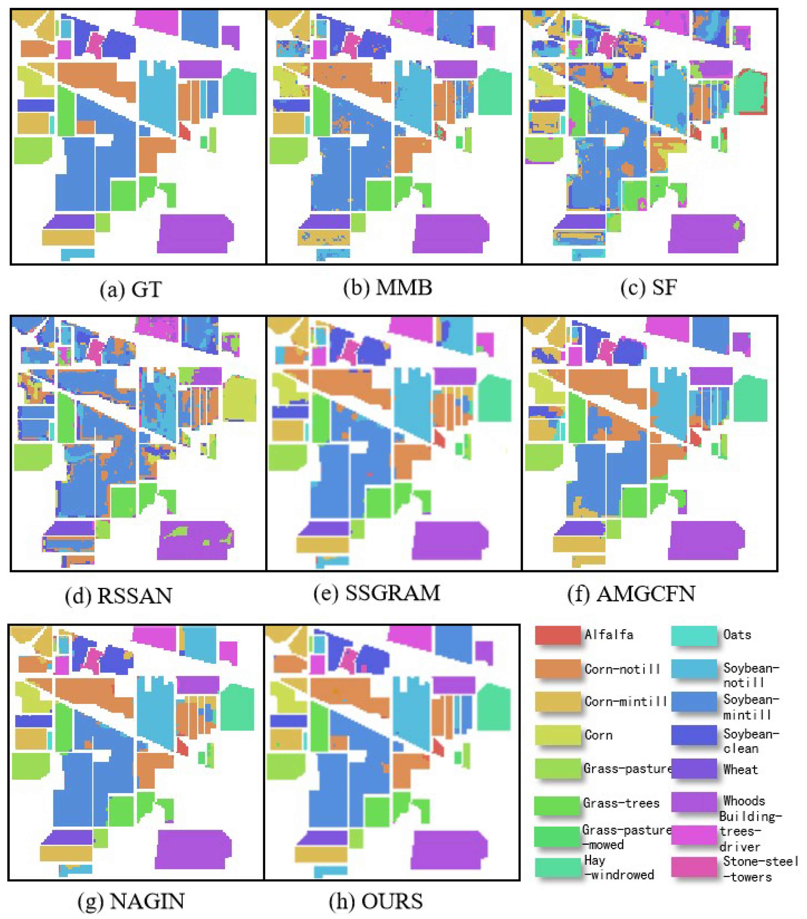
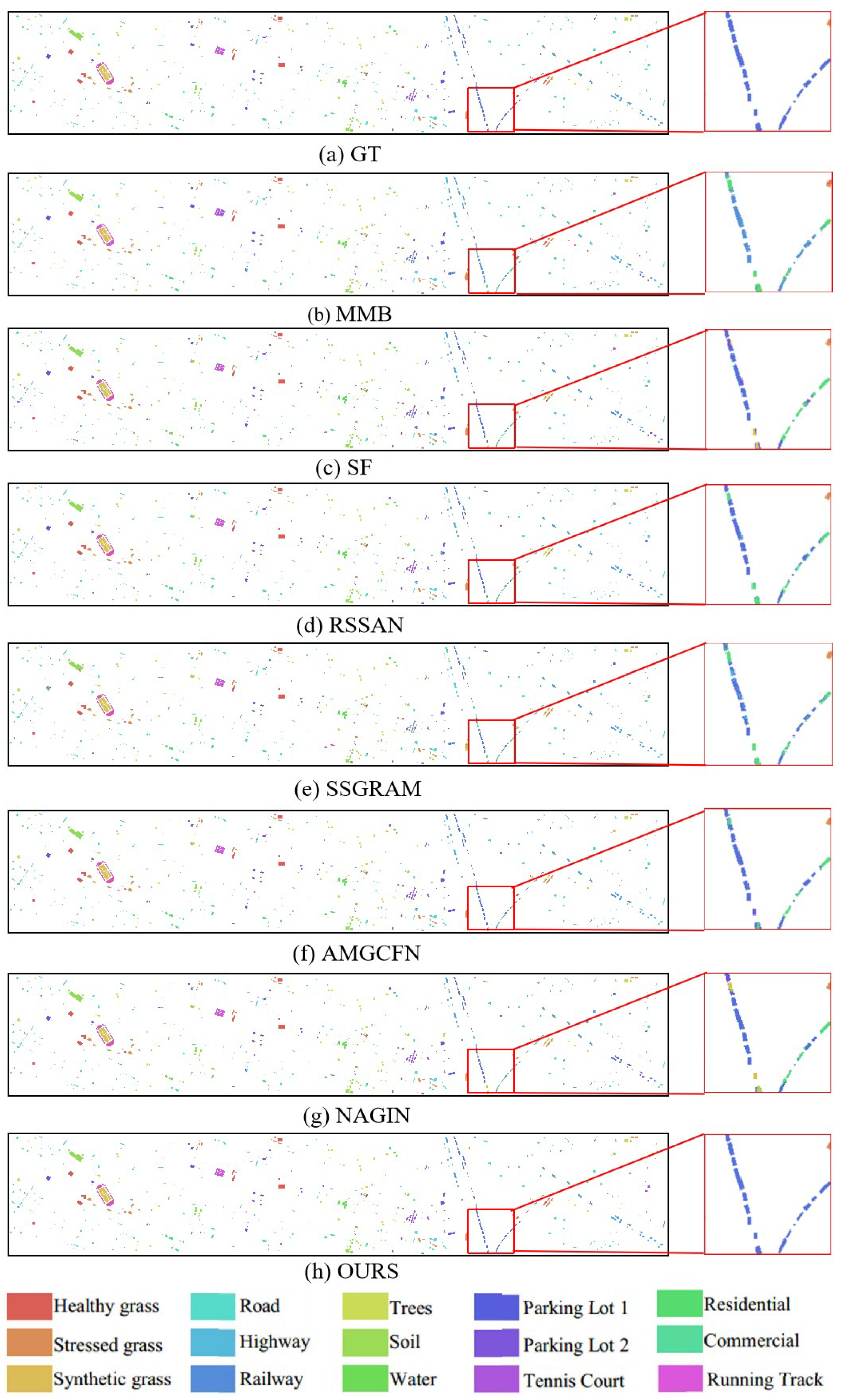
Figure 7, Figure 8 and Figure 9 demonstrate the visual maps of IP, UH2013, and SA, respectively. The Transformer-based method SF and the CNN-based method RSSAN performed poorly, the receptive field defect of RSSAN and the insufficient cross-layer feature fusion of SF led to a large amount of pepper noise. The classification of pixel points also contains many errors and is distributed relatively densely at the edge and inside the entities. The classification effect of Mamba-based method MMB is better than that of SF and RSSAN. However, MMB pays excessive attention to global information and has insufficient modeling of local details, resulting in dotted noise in the visual map. The classification accuracy of the GNN-based method SSGRAM is second only to GLFFEN. However, due to the insufficient ability of local feature extraction, the edge information of ground objects is lost. The hybrid model method AMGCFN takes into account both global and local information. However, the simple fusion strategy cannot fully combine global and local features, resulting in block-wide classification errors in its visual map. Interestingly, while the NAGIN enhances the model’s ability to discriminate heterogeneous features through adaptive neighborhood graph isomorphism for feature extraction and relational reasoning, it also introduces over-smoothing effects, leading to blurred inter-category boundaries in the visualized high-dimensional embedding space. Compared with all comparison methods, GLFFEN achieves the highest classification accuracy and the smoothest visual map. In addition, GLFFEN demonstrates clear edges and less error on the IP dataset, rich detail and texture information on the UH2013 dataset, and the highest smoothness on the SA dataset.

4.3.3. Efficiency Analysis

To verify the efficiency of GLFFEN, we recorded the running time and computational load (FLOPs) of all comparison algorithms. The test results are shown in

Table 7. Results of efficiency experiments.

Methods	Running Time (s)						Complexity (FLOPs)
	IP		UH2013		SA
	Train	Test	Train	Test	Train	Test
MMB	68.63	2.31	39.32	2.94	76.48	2.29	0.96 G
SF	460.78	42.36	176.24	106.34	490.58	240.14	1.50 G
RSSAN	125.32	4.28	43.75	12.18	89.03	9.25	0.85 G
SSGRAM	138.56	7.11	95.15	13.45	189.36	16.35	1.88 G
AMGCFN	153.22	5.34	78.65	11.22	184.12	6.92	6.32 G
NAGIN	129.65	6.25	88.56	10.55	168.45	10.56	1.74 G
OURS	98.56	3.15	59.35	4.98	103.96	6.38	0.91 G

. It can be seen that the recent work, while improving the classification accuracy, has also brought a heavy computational burden. This problem becomes more prominent when using a dual-backbone network with a CNN-GNN fusion architecture (e.g., AMGCFN), but GLFFEN achieves SOTA classification results with an extremely low computational burden through a reasonable fusion strategy (MAF module) and by giving up low-contribution node connectivity. RSSAN has the lowest FLOPs, but this simple residual network structure makes the classification accuracy not ideal. MMB has high operational efficiency, but its computational burden is still higher than that of GLFFEN, and there is a gap in classification accuracy compared with advanced dual-backbone network architectures. Compared with all other methods, GLFFEN significantly reduces the adjacency matrix dimension of GNN by using superpixel segmentation and the discarding strategy of low-contribution edges. Our GLFFEN only requires a computational cost of 0.91 G FLOPs to achieve SOTA classification. While taking into account the computational complexity, the SSFAM we designed highly adopts parallelized dense matrix multiplication and an extremely low number of parameters, which means that GLFFEN only needs less time to generate classification results. Therefore, the advantages of classification accuracy and operational efficiency also indicate that our GLFFEN has broad prospects for industrial application.

5. Discussion

Section 5.1 shows the parameter sensitivity analysis. Section 5.2 presents the stability assessment under varying training set sizes. Section 5.3 presents the ablation study. Section 5.4 introduces the loss function analysis.

5.1. Parameter Sensitivity Analysis

The proposed GLFFEN framework involves three crucial hyperparameters: convolutional kernel size (k), number of attention heads, and dropout rate. In our method, the kernel size governs the receptive field of the CNN component. The number of attention heads determines the parallel learning pathways in the multi-head attention mechanism, where each head independently learns distinct attention patterns to capture node relationships from diverse perspectives. Dropout regularization randomly omits a subset of neuronal connections during training to prevent overfitting.

For kernel size configuration, we balance receptive field coverage against computational complexity by testing combinations of (3, 3), (3, 5), (5, 3), and (5, 5) for the two consecutive convolutional layers. As shown in

Table 8. Classification performance of GLFFEN with different kernel size k on each dataset. (m, n) means that the convolution kernel of the first and second convolution layers are m × n.

Kernel Size	(3, 3)	(3, 5)	(5, 3)	(5, 5)
IP	93.74	97.97	96.68	95.98
UH2013	96.34	96.11	92.45	93.33
SA	95.49	97.93	94.33	94.29

, the configuration with k = (3, 5) achieves peak OA scores on IP and SA datasets while delivering second-best results on UH2013. Regarding attention heads, we evaluate configurations ranging from 1 to 5. For dropout rate, we examine values from 0.1 to 0.5 with 0.1 increments. Comprehensive experiments analyze the interaction between these two parameters. Figure 10 demonstrates that the combination of 4 attention heads with a 0.4 dropout rate yields optimal OA across all three datasets. Consequently, these values (4 attention heads, 0.4 dropout rate) become the default configuration for GLFFEN.

5.2. Stability Assessment Under Varying Training Set Sizes

Variations in training-sample quantities typically induce performance fluctuations across algorithms. To assess the stability of our GLFFEN framework under different data volumes, we performed comparative experiments involving seven benchmark methods across three distinct training set configurations. For each dataset, the per-class training samples were configured at 10, 15, 20, 25, and 30 instances, respectively. Figure 11 illustrates the progression of Overall Accuracy (OA) metrics relative to training-sample increments across all datasets. The results reveal a consistent monotonic improvement in OA values corresponding to increased training samples. Particularly noteworthy is GLFFEN’s persistent attainment of peak OA performance across all experimental conditions. Additionally, while certain approaches (including SF and RSSAN) display pronounced OA oscillations with changing sample sizes, GLFFEN maintains substantially smoother performance trajectories. These observations collectively verify the framework’s enhanced robustness and generalization capacity.

5.3. Ablation Study

In the ablation experiment, we considered the combination of four factors for research, namely the GA branch, the single-layer SSFAM, the SSFA branch, and the MAF module. As shown in

Table 9. Results of ablation experiment on IP dataset. Numbers in bold denote the best value.

Methods	SSFAM	SSFA Branch	GA Branch	MAF Module	OA (%)	AA (%)	KAPPA
GLFFEN	√	×	×	×	83.48	86.09	85.19
	×	√	×	×	89.64	91.15	90.78
	×	×	√	×	91.06	92.43	91.84
	√	×	√	√	93.49	95.17	94.03
	×	√	√	×	94.11	96.56	94.37
	×	√	√	√	97.97	98.04	97.38

, we construct the following variants with different component combinations. In the experimental results, the complete GLFFEN achieves the optimal values on all three metrics of OA, AA, and KAPPA.

The notable performance improvement achieved by fusing the SSFA and GA branches, despite their modest individual performance, can be attributed to their inherent complementarity in feature representation. The SSFA branch excels at capturing fine-grained pixel-level details and local spectral variations through its self-attention mechanisms, but may lack robust global contextual understanding. Conversely, the GA branch provides strong topological reasoning and long-range dependency modeling at the superpixel level, yet inevitably suffers from information loss during the superpixel segmentation process.The MAF module serves as an intelligent integration mechanism that adaptively weights these complementary features based on local context—assigning higher weights to GA features in homogeneous areas and prioritizing SSFA features in regions with complex textures or boundary details. This synergistic fusion creates a more comprehensive feature representation than either branch could achieve independently, effectively explaining the significant performance gain observed in Table 9.

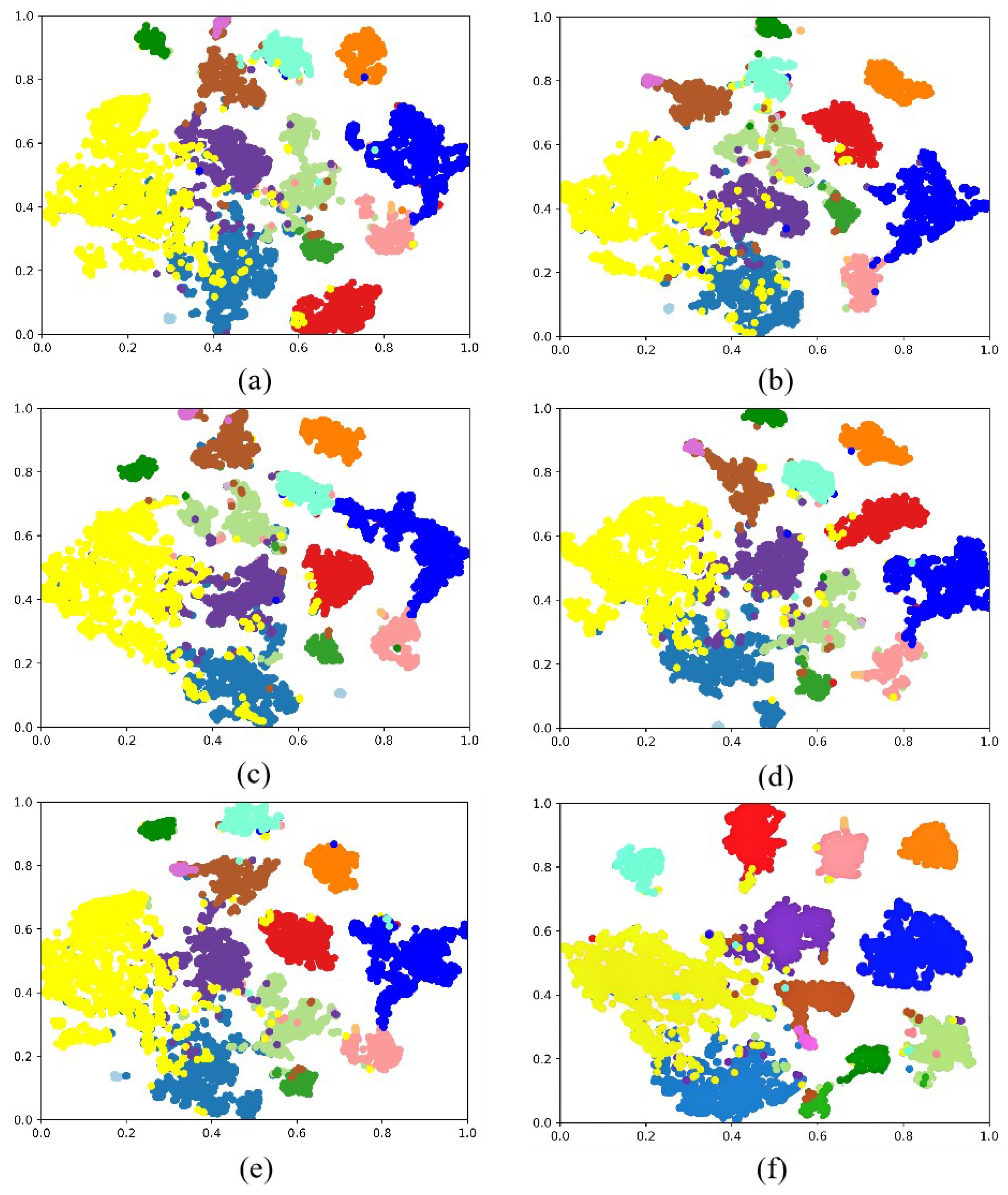
To demonstrate the effectiveness of each GLFFEN module more intuitively, we use t-sne to show the feature distribution of different module combinations, and the results are shown in Figure 12. It can be clearly seen that the proposed GLFFEN learning has the most concentrated features and the highest feature separability. Therefore, the module design of GLFFEN is reasonable and necessary.

5.4. Loss Function Analysis

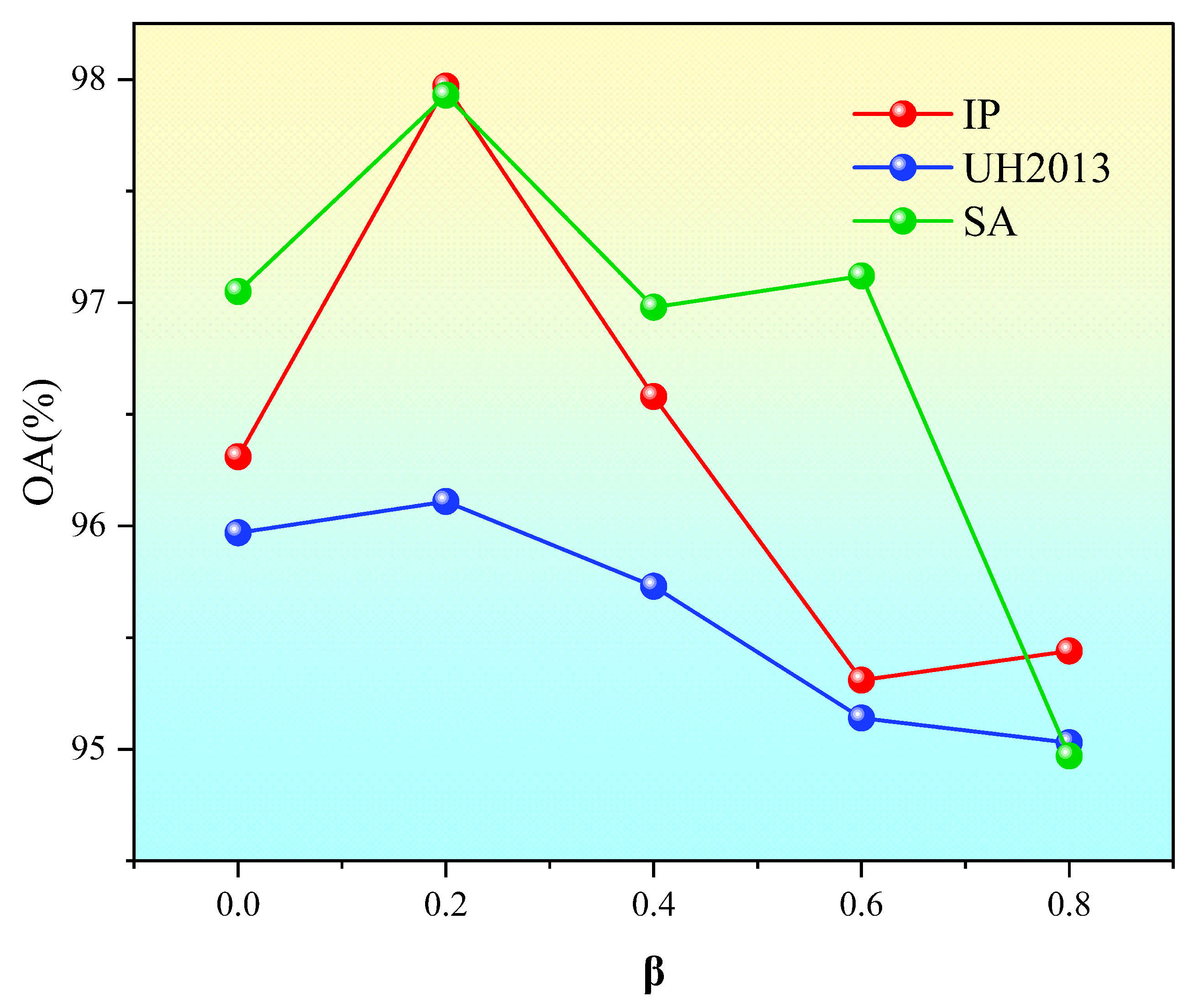
Our loss function incorporates both reconstruction loss and identity loss. To determine how different loss configurations affect the model performance, we systematically examine the coefficients $\alpha$ (for reconstruction loss) and $\beta$ (for identity loss). Since the constraint $\alpha$ + $\beta$ = 1 must be satisfied, the key lies in identifying the optimal value for the identity loss coefficient $\beta$. Accordingly, $\beta$ is set to 0, 0.2, 0.4, 0.6, and 0.8 to analyze its impact on the Overall Accuracy (OA). Notably, as shown in Figure 13, when $\beta$ = 0 (indicating no identity loss is introduced), the OA values across all three datasets fail to reach their maximum. At $\beta$ = 0.2, the highest OA is achieved on all three datasets. However, as $\beta$ continues to increase, the OA values decline to varying degrees across the datasets. This occurs because an excessive identity loss overemphasizes feature preservation constraints, causing the model to become excessively conservative in replicating input features. This consequently diminishes its capacity to learn high-level discriminative features and leads to overly smoothed feature representations with insufficient inter-class distinction. Ultimately, these effects make it difficult for the classifier to effectively separate different categories in the compressed feature space. This experiment proves the necessity of introducing identity loss into the loss function.

6. Conclusions

This paper proposes GLFFEN, a global–local feature fusion enhancement network for hyperspectral image classification. By combining the global and local feature extraction capabilities of GNN and CNN, more comprehensive and detailed classification information can be obtained. We design a GNN based on superpixel segmentation and multi-head attention mechanism as a GA branch for extracting global features. In addition, we propose SSFAM to focus more effectively on the local spatial–spectral features. By the way, the MAF module is ingeniously designed and used for the fusion of global–local feature self-weighting, which ensures the automatic adjustment of the fusion strategy for different ground object types under different datasets. Comparison experiments on three well-known HSI datasets show that our GLFFEN has a significant advantage over the other six SOTA methods in terms of the classification effect.

Although the proposed GLFFEN framework is competitive, this study acknowledges certain limitations. This model is still inherently constrained by its reliance on the quality of superpixel segmentation. In addition, the parallel dual-branch architecture still brings about relatively high computational complexity. These aspects highlight the key directions for future research, including exploring unsegmented graph construction, developing more adaptive and in-depth feature fusion interaction mechanisms, and simplifying model structures to enhance computational efficiency.

References

1. Zhang, H.; Liu, H.; Yang, R.; Wang, W.; Luo, Q.; Tu, C. Hyperspectral Image Classification Based on Double-Branch Multi-Scale Dual-Attention Network. Remote Sens. 2024, 16, 2051. [Google Scholar] [CrossRef]
2. Nasrabadi, N.M. Hyperspectral target detection: An overview of current and future challenges. IEEE Signal Process. Mag. 2013, 31, 34–44. [Google Scholar] [CrossRef]
3. Ghamisi, P.; Yokoya, N.; Li, J.; Liao, W.; Liu, S.; Plaza, J.; Rasti, B.; Plaza, A. Advances in hyperspectral image and signal processing: A comprehensive overview of the state of the art. IEEE Geosci. Remote Sens. Mag. 2017, 5, 37–78. [Google Scholar] [CrossRef]
4. Ghamisi, P.; Maggiori, E.; Li, S.; Souza, R.; Tarablaka, Y.; Moser, G.; De Giorgi, A.; Fang, L.; Chen, Y.; Chi, M.; et al. New frontiers in spectral-spatial hyperspectral image classification: The latest advances based on mathematical morphology, Markov random fields, segmentation, sparse representation, and deep learning. IEEE Geosci. Remote Sens. Mag. 2018, 6, 10–43. [Google Scholar] [CrossRef]
5. Yokoya, N.; Grohnfeldt, C.; Chanussot, J. Hyperspectral and multispectral data fusion: A comparative review of the recent literature. IEEE Geosci. Remote Sens. Mag. 2017, 5, 29–56. [Google Scholar] [CrossRef]
6. Bioucas-Dias, J.M.; Plaza, A.; Camps-Valls, G.; Scheunders, P.; Nasrabadi, N.; Chanussot, J. Hyperspectral remote sensing data analysis and future challenges. IEEE Geosci. Remote Sens. Mag. 2013, 1, 6–36. [Google Scholar] [CrossRef]
7. Ren, L.; Zhao, L.; Wang, Y. A superpixel-based dual window RX for hyperspectral anomaly detection. IEEE Geosci. Remote Sens. Lett. 2019, 17, 1233–1237. [Google Scholar] [CrossRef]
8. Rajabi, R.; Zehtabian, A.; Singh, K.D.; Tabatabaeenejad, A.; Ghamisi, P.; Homayouni, S. Hyperspectral imaging in environmental monitoring and analysis. Front. Environ. Sci. 2024, 11, 1353447. [Google Scholar] [CrossRef]
9. Caballero, D.; Calvini, R.; Amigo, J.M. Hyperspectral imaging in crop fields: Precision agriculture. In Data Handling in Science and Technology; Elsevier: Amsterdam, The Netherlands, 2019; Volume 32, pp. 453–473. [Google Scholar]
10. Xu, Y.; Zhang, L.; Du, B.; Zhang, L. Hyperspectral anomaly detection based on machine learning: An overview. IEEE J. Sel. Top. Appl. Earth Obs. Remote Sens. 2022, 15, 3351–3364. [Google Scholar] [CrossRef]
11. Yang, X.; Yu, Y. Estimating soil salinity under various moisture conditions: An experimental study. IEEE Trans. Geosci. Remote Sens. 2017, 55, 2525–2533. [Google Scholar] [CrossRef]
12. Amini, S.; Homayouni, S.; Safari, A.; Darvishsefat, A.A. Object-based classification of hyperspectral data using Random Forest algorithm. Geo-Spat. Inf. Sci. 2018, 21, 127–138. [Google Scholar] [CrossRef]
13. Guo, Y.; Han, S.; Li, Y.; Zhang, C.; Bai, Y. K-Nearest Neighbor combined with guided filter for hyperspectral image classification. Procedia Comput. Sci. 2018, 129, 159–165. [Google Scholar] [CrossRef]
14. Zhang, B.; Li, S.; Jia, X.; Gao, L.; Peng, M. Adaptive Markov random field approach for classification of hyperspectral imagery. IEEE Geosci. Remote Sens. Lett. 2011, 8, 973–977. [Google Scholar] [CrossRef]
15. Li, W.; Prasad, S.; Fowler, J.E. Hyperspectral image classification using Gaussian mixture models and Markov random fields. IEEE Geosci. Remote Sens. Lett. 2013, 11, 153–157. [Google Scholar] [CrossRef]
16. Melgani, F.; Bruzzone, L. Classification of hyperspectral remote sensing images with support vector machines. IEEE Trans. Geosci. Remote Sens. 2004, 42, 1778–1790. [Google Scholar] [CrossRef]
17. Islam, M.R.; Islam, M.T.; Uddin, M.P.; Ulhaq, A. Improving hyperspectral image classification with compact multi-branch deep learning. Remote Sens. 2024, 16, 2069. [Google Scholar] [CrossRef]
18. Zhou, P.; Han, J.; Cheng, G.; Zhang, B. Learning compact and discriminative stacked autoencoder for hyperspectral image classification. IEEE Trans. Geosci. Remote Sens. 2019, 57, 4823–4833. [Google Scholar] [CrossRef]
19. Li, Z.; Xue, Z.; Jia, M.; Nie, X.; Wu, H.; Zhang, M.; Su, H. DEMAE: Diffusion enhanced masked autoencoder for hyperspectral image classification with few labeled samples. IEEE Trans. Geosci. Remote Sens. 2024, 62, 5527616. [Google Scholar] [CrossRef]
20. Hang, R.; Liu, Q.; Hong, D.; Ghamisi, P. Cascaded recurrent neural networks for hyperspectral image classification. IEEE Trans. Geosci. Remote Sens. 2019, 57, 5384–5394. [Google Scholar] [CrossRef]
21. Hong, D.; Gao, L.; Yao, J.; Zhang, B.; Plaza, A.; Chanussot, J. Graph convolutional networks for hyperspectral image classification. IEEE Trans. Geosci. Remote Sens. 2020, 59, 5966–5978. [Google Scholar] [CrossRef]
22. Wu, K.; Zhan, Y.; An, Y.; Li, S. Multiscale feature search-based graph convolutional network for hyperspectral image classification. Remote Sens. 2024, 16, 2328. [Google Scholar] [CrossRef]
23. Sun, L.; Zhao, G.; Zheng, Y.; Wu, Z. Spectral–spatial feature tokenization transformer for hyperspectral image classification. IEEE Trans. Geosci. Remote Sens. 2022, 60, 5522214. [Google Scholar] [CrossRef]
24. Li, Y.; Luo, Y.; Zhang, L.; Wang, Z.; Du, B. MambaHSI: Spatial-spectral mamba for hyperspectral image classification. IEEE Trans. Geosci. Remote Sens. 2024, 62, 5524216. [Google Scholar] [CrossRef]
25. Yang, A.; Li, M.; Ding, Y.; Fang, L.; Cai, Y.; He, Y. Graphmamba: An efficient graph structure learning vision mamba for hyperspectral image classification. IEEE Trans. Geosci. Remote Sens. 2024, 62, 5537414. [Google Scholar] [CrossRef]
26. Hu, W.; Huang, Y.; Wei, L.; Zhang, F.; Li, H. Deep convolutional neural networks for hyperspectral image classification. J. Sensors 2015, 2015, 258619. [Google Scholar] [CrossRef]
27. Hamida, A.B.; Benoit, A.; Lambert, P.; Amar, C.B. 3-D deep learning approach for remote sensing image classification. IEEE Trans. Geosci. Remote Sens. 2018, 56, 4420–4434. [Google Scholar] [CrossRef]
28. Zhu, M.; Jiao, L.; Liu, F.; Yang, S.; Wang, J. Residual spectral–spatial attention network for hyperspectral image classification. IEEE Trans. Geosci. Remote Sens. 2020, 59, 449–462. [Google Scholar] [CrossRef]
29. Hong, D.; Han, Z.; Yao, J.; Gao, L.; Zhang, B.; Plaza, A.; Chanussot, J. SpectralFormer: Rethinking hyperspectral image classification with transformers. IEEE Trans. Geosci. Remote Sens. 2021, 60, 5518615. [Google Scholar] [CrossRef]
30. Yang, A.; Li, M.; Ding, Y.; Hong, D.; Lv, Y.; He, Y. GTFN: GCN and transformer fusion network with spatial-spectral features for hyperspectral image classification. IEEE Trans. Geosci. Remote Sens. 2023, 61, 6600115. [Google Scholar] [CrossRef]
31. Paul, B.; Fattah, S.A.; Rajib, A.; Saquib, M. SSGRAM: 3D Spectral-Spatial Feature Network Enhanced by Graph Attention Map for Hyperspectral Image Classification. IEEE Trans. Geosci. Remote Sens. 2025, 63, 5516715. [Google Scholar] [CrossRef]
32. Wang, N.; Yang, A.; Cui, Z.; Ding, Y.; Xue, Y.; Su, Y. Capsule Attention Network for Hyperspectral Image Classification. Remote Sens. 2024, 16, 4001. [Google Scholar] [CrossRef]
33. Lee, H.; Kwon, H. Going deeper with contextual CNN for hyperspectral image classification. IEEE Trans. Image Process. 2017, 26, 4843–4855. [Google Scholar] [CrossRef]
34. Ahmad, M.; Mazzara, M.; Distifano, S. Importance of Disjoint Sampling in Conventional and Transformer Models for Hyperspectral Image Classification. arXiv 2024, arXiv:2404.14944. [Google Scholar] [CrossRef]
35. Hu, H.; Yao, M.; He, F.; Zhang, F. Graph neural network via edge convolution for hyperspectral image classification. IEEE Geosci. Remote Sens. Lett. 2021, 19, 5508905. [Google Scholar] [CrossRef]
36. Wang, N.; Cui, Z.; Li, A.; Xue, Y.; Wang, R.; Nie, F. Multi-order graph based clustering via dynamical low rank tensor approximation. Neurocomputing 2025, 647, 130571. [Google Scholar] [CrossRef]
37. Zhang, J.; Tu, B.; Liu, B.; Li, J.; Plaza, A. Hyperspectral Image Classification via Neighborhood Adaptive Graph Isomorphism Network. IEEE Trans. Geosci. Remote Sens. 2025, 63, 5515717. [Google Scholar] [CrossRef]
38. Xu, Y.; Du, B.; Zhang, F.; Zhang, L. Hyperspectral image classification via a random patches network. ISPRS J. Photogramm. Remote Sens. 2018, 142, 344–357. [Google Scholar] [CrossRef]
39. Zhao, L.; Li, J.; Luo, W.; Ouyang, E.; Wu, J.; Zhang, G.; Li, W. Purified contrastive learning with global and local representation for hyperspectral image classification. IEEE Trans. Geosci. Remote Sens. 2024, 62, 5520414. [Google Scholar] [CrossRef]
40. LeCun, Y.; Bengio, Y.; Hinton, G. Deep learning. Nature 2015, 521, 436–444. [Google Scholar] [CrossRef]
41. Wang, N.; Cui, Z.; Li, A.; Wang, R.; Nie, F. Multi-view Clustering based on Doubly Stochastic Graph. Signal Process. 2025, 238, 110144. [Google Scholar] [CrossRef]
42. Wang, N.; Cui, Z.; Lan, Y.; Zhang, C.; Xue, Y.; Su, Y.; Li, A. Large-Scale Hyperspectral Image-Projected Clustering via Doubly Stochastic Graph Learning. Remote Sens. 2025, 17, 1526. [Google Scholar] [CrossRef]
43. Yu, L.; Peng, J.; Chen, N.; Sun, W.; Du, Q. Two-Branch Deeper Graph Convolutional Network for Hyperspectral Image Classification. IEEE Trans. Geosci. Remote Sens. 2023, 61, 5506514. [Google Scholar] [CrossRef]
44. Dong, Y.; Liu, Q.; Du, B.; Zhang, L. Weighted feature fusion of convolutional neural network and graph attention network for hyperspectral image classification. IEEE Trans. Image Process. 2022, 31, 1559–1572. [Google Scholar] [CrossRef]
45. Wang, J.; Li, W.; Gao, Y.; Zhang, M.; Tao, R.; Du, Q. Hyperspectral and SAR image classification via multiscale interactive fusion network. IEEE Trans. Neural Netw. Learn. Syst. 2022, 34, 10823–10837. [Google Scholar] [CrossRef]
46. Liu, X.; Ng, A.H.M.; Ge, L.; Lei, F.; Liao, X. Multi-branch fusion: A multi-branch attention framework by combining graph convolutional network and CNN for hyperspectral image classification. IEEE Trans. Geosci. Remote Sens. 2024, 62, 5528817. [Google Scholar]
47. Zhang, X.; Chew, S.E.; Xu, Z.; Cahill, N.D. SLIC superpixels for efficient graph-based dimensionality reduction of hyperspectral imagery. In Proceedings of the Algorithms and Technologies for Multispectral, Hyperspectral, and Ultraspectral Imagery XXI, Baltimore, MD, USA, 21–23 April 2015; SPIE: Nuremberg, Germany, 2015; Volume 9472, pp. 92–105. [Google Scholar]
48. Vaswani, A.; Shazeer, N.; Parmar, N.; Uszkoreit, J.; Jones, L.; Gomez, A.N.; Kaiser, Ł.; Polosukhin, I. Attention is all you need. Adv. Neural Inf. Process. Syst. 2017, 30, 6000–6010. [Google Scholar]
49. Li, L.; Yin, J.; Jia, X.; Li, S.; Han, B. Joint spatial–spectral attention network for hyperspectral image classification. IEEE Geosci. Remote Sens. Lett. 2020, 18, 1816–1820. [Google Scholar] [CrossRef]
50. Peng, Y.; Zhang, Y.; Tu, B.; Li, Q.; Li, W. Spatial–spectral transformer with cross-attention for hyperspectral image classification. IEEE Trans. Geosci. Remote Sens. 2022, 60, 5537415. [Google Scholar] [CrossRef]
51. Fu, J.; Liu, J.; Tian, H.; Li, Y.; Bao, Y.; Fang, Z.; Lu, H. Dual attention network for scene segmentation. In Proceedings of the IEEE/CVF Conference on Computer Vision and Pattern Recognition, Long Beach, CA, USA, 16–17 June 2019; pp. 3146–3154. [Google Scholar]
52. Zhou, H.; Luo, F.; Zhuang, H.; Weng, Z.; Gong, X.; Lin, Z. Attention multihop graph and multiscale convolutional fusion network for hyperspectral image classification. IEEE Trans. Geosci. Remote Sens. 2023, 61, 5508614. [Google Scholar] [CrossRef]
Figure 1. The mechanisms of GNN and CNN.
Remotesensing 17 03705 g001
Figure 2. The categories of ground objects in HSIs often exhibit non-uniformity in space, which makes it difficult for the local features extracted by CNN based on regular grids to generalize to all regions of the entire image.
Remotesensing 17 03705 g002
Figure 3. The overall framework of the proposed GLFFEN.
Remotesensing 17 03705 g003
Figure 4. The mechanisms of SLIC: after SLIC, the nodes of the GNN change from pixels to superpixels formed by the aggregation of pixels.
Remotesensing 17 03705 g004
Figure 5. The network architecture of SSFAM.
Remotesensing 17 03705 g005
Figure 6. The proposed MAF module.
Remotesensing 17 03705 g006
Figure 7. Visual maps of the results on the IP dataset.
Remotesensing 17 03705 g007
Figure 8. Visual maps of the results on the UH2013 dataset.
Remotesensing 17 03705 g008
Figure 9. Visual maps of the results on the SA dataset.
Remotesensing 17 03705 g009
Figure 10. Sensitivity of GLFFEN in different parameter settings (i.e., number of attention heads and dropout rate) on (a) IP, (b) UH2013, and (c) SA.
Remotesensing 17 03705 g010
Figure 11. OA for different proportions of training samples on the three datasets. (ac) OA curves in the IP, UH2013, and SA datasets, respectively.
Remotesensing 17 03705 g011
Figure 12. The visual feature distributions using t-sne: (a) SSFAM; (b) SSFA branch; (c) GA branch; (d) SSFAM + GA branch + MAF module; (e) SSFA branch+GA branch; (f) GLFFEN.
Remotesensing 17 03705 g012
Figure 13. The influence of different identity loss coefficients β on the OA value on three datasets: when β = 0, it indicates no identity loss.
Remotesensing 17 03705 g013