Highlights
What are the main findings?
- A strategy integrating the strengths of pixel- and object-based classification was developed, achieving high classification performance and fine differentiation of coastal wetlands.
- A set of composite feature variables was constructed and optimized that effectively captures the differential dynamic characteristics of coastal wetland types.
What are the implication of the main finding?
- The proposed classification strategy effectively addresses key challenges in coastal wetland mapping, establishing a reliable framework for large-scale, high-precision applications.
- Fine-grained wetland classification characterizes ecological functional distinctions among wetland types, facilitating targeted management of coastal wetlands.
Abstract
Accurate and detailed mapping of coastal wetlands is essential for effective wetland resource management. However, due to periodic tidal inundation, frequent cloud cover, and spectral similarity of land cover types, reliable coastal wetland classification methods remain limited. To address these issues, we developed an integrated pixel- and object-based hierarchical classification strategy based on multi-source remote sensing data to achieve fine-grained coastal wetland classification on Google Earth Engine. With the random forest classifier, pixel-level classification was performed to classify rough wetland and non-wetland types, followed by object-based classification to differentiate artificial and natural attributes of water bodies. In this process, multi-dimensional features including water level, phenology, variation, topography, geography, and geometry were extracted from Sentinel-1/2 time-series images, topographic data and shoreline data, which can fully capture the variability and dynamics of coastal wetlands. Feature combinations were then optimized through Recursive Feature Elimination and Jeffries–Matusita analysis to ensure the model’s ability to distinguish complex wetland types while improving efficiency. The classification strategy was applied to typical coastal wetlands in central Jiangsu in 2020 and finally generated a 10 m wetland map including 7 wetland types and 3 non-wetland types, with an overall accuracy of 92.50% and a Kappa coefficient of 0.915. Comparative analysis with existing datasets confirmed the reliability of this strategy, particularly in extracting intertidal mudflats, salt marshes, and artificial wetlands. This study can provide a robust framework for fine-grained wetland mapping and support the inventory and conservation of coastal wetland resources.
1. Introduction
Coastal wetlands, located in the transitional zone between the land and sea, are recognized as one of the most productive and valuable ecosystems, playing a crucial role in maintaining biodiversity, climate regulation, coastal protection, and carbon storage [1,2]. However, due to intensified human impact and climate change, such as pollution, sea reclamation, rising sea levels, extreme weather events, and so on [3,4], the intra-annual and inter-annual changes in coastal wetlands have become more frequent and complex, leading to increasing fragmentation and severe degradation of their ecosystem services and functions [5,6]. Given the urgent need to monitor biodiversity changes, prevent wetland degradation, and support precise ecological restoration, it is essential to conduct high-accuracy, large-scale, and annual mapping of coastal wetland composition.
In recent years, satellite remote sensing has become a powerful tool for coastal wetland monitoring due to its extensive coverage and repeatable observation capabilities. A range of large-scale wetland thematic datasets have been created using remote sensing data, including the Global Wetland Map with a Fine Classification System (GWL_FCS30) [7], the National Wetland Mapping Dataset of China (CAS_Wetlands) [8], the Global Tidal Flat Mapping Product (GTF) [9], and the Global Mangrove Forests Product [10]. Under the combined driving forces of natural factors and human activities, coastal wetlands often undergo rapid land cover changes within short timeframes, including accelerated vegetation loss, continuous encroachment of built-up areas into wetland spaces, and so on [11]. Nevertheless, these datasets are often constrained by limitations such as insufficient spatial resolution and discontinuous spatiotemporal coverage, making them inadequate to meet the stringent requirements for high accuracy and timeliness in dynamic biodiversity monitoring and precise wetland degradation assessment. It is particularly noteworthy that the surface cover status of coastal wetlands is highly dependent on periodic tidal inundation, yet most datasets lack effective characterization of tidal dynamics, leading to widespread misclassification in frequently inundated areas such as intertidal zones [12]. Furthermore, the classification systems of these datasets are often neither unified nor sufficiently detailed, failing to adequately distinguish ecologically significant fine-grained types in coastal wetlands, such as specific vegetation communities, tidal flats, and water bodies [13,14]. These limitations severely restrict their utility for analyzing wetland ecological processes and supporting refined management decisions. Consequently, the development of more precise and accurate coastal wetland mapping methods remains a challenge.
The dynamic nature of coastal wetlands, influenced by tidal cycles, coastal vegetation phenology, natural hazards and human impacts, causes significant spatiotemporal uncertainties in classification, which are further exacerbated by limitations in remote sensing image quality [15,16]. Traditional coastal wetland classification methods often rely on images captured at specific dates (e.g., high/low tide moments) or single composite images over a certain period, since high/low tide images can effectively distinguish coastal wetlands from inland landscapes [17], while images selected during specific phenological windows can enhance the separability of coastal wetland vegetation [18,19]. However, these methods heavily depend on manual screening based on prior knowledge, lacking automation and being labor-intensive and time-consuming [20,21,22]. Also, these methods are difficult to apply on a large scale since they often overlook the detailed temporal dynamics of coastal wetland features [14]. Moreover, under extreme weather conditions, factors such as cloud cover and satellite revisit intervals limit the availability of usable images for specific coastal wetland areas, particularly for optical imagery [23,24]. To address these challenges, many studies have turned to integrating multi-source, heterogeneous, and multi-temporal remote sensing data to capture the dynamic spatiotemporal characteristics of coastal wetlands for classification [25]. On the one hand, Synthetic Aperture Radar (SAR) sensors, which support all-weather and day-night observations, can be combined with optical data to increase observation frequency and provide complementary surface information, thereby improving classification accuracy [26]. On the other hand, leveraging time-series imagery, by masking low-quality pixels and retaining high-quality ones, can reduce imprecision of images and provide richer temporal feature variables for wetland classification [27]. In comparison, Sentinel data, with its complementary imaging satellite missions (optical and radar), high spatial resolution, and short revisit cycles, is more widely applied. These characteristics enable researchers to construct long-term, pixel-level, high-quality data stacks, better capturing tidal variations and vegetation phenology in coastal areas [28,29].
The necessity of storing and processing a large amount of data has posed certain technical bottlenecks for remote sensing applications based on multi-source, heterogeneous, and multi-temporal data [30]. In recent years, the emergence of the Google Earth Engine (GEE) cloud platform has revolutionized large-scale, long-term remote sensing time-series analysis. Leveraging its powerful cloud computing capabilities and massive data storage infrastructure, GEE provides built-in support for machine learning algorithms, enabling efficient processing of geospatial big data [31]. This platform has been widely applied to multi-scale mapping of coastal wetlands, including aquaculture ponds [32], tidal flats [33], Spartina alterniflora [34], and so on across varying spatiotemporal scales. The development of novel classification strategies integrating multi-source and multi-temporal remote sensing data through GEE holds significant potential to substantially enhance processing efficiency and accuracy, demonstrating tremendous promise for obtaining more reliable results in near-real-time Earth observation applications.
To enhance the separability of coastal wetland categories and reduce classification uncertainty in complex and fragmented coastal wetland landscapes, it is essential to integrate multiple types of feature variables from different perspectives, such as spectral, radar, topographic, and phenological features [35,36]. However, the combination of multi-source and multi-temporal remote sensing data generates an excessive number of feature variables, inevitably leading to redundancy among these features. As the dimension of feature variables increases, the computational complexity of classification models rises significantly, which may lead to overfitting [37]. Fu et al. [38] combined Recursive Feature Elimination (RFE) with the random forest algorithm to create an optimal feature variable set for regional marsh vegetation identification, improving model efficiency and stability. Similarly, Zhao et al. [39] integrated multiple feature selection algorithms, including Laplacian score, distance correlation, and Jeffries–Matusita with adaptive weighting, providing robust dimensionality reduction capabilities. This method not only maintained wetland classification accuracy but also effectively reduced computational costs. Evidently, feature selection is important for balancing classification efficiency and accuracy, serving as a key factor in improving wetland classification performance.
To date, machine learning algorithms such as random forest, support vector machines and neural networks have been widely applied in wetland classification studies [40,41], which have primarily focused on national or regional scales, relying on pixel-level features to identify wetland types. Pixel-based classification methods are capable of capturing high-resolution details, making them suitable for fine-scale wetland classification. However, in coastal areas with high local heterogeneity, the widespread presence of phenomena, such as “the different objects with similar spectra” and “the same object with different spectra”, makes accurate classification challenging when relying solely on pixel-level features [42,43]. In contrast, object-based wetland classification methods generate image objects by segmenting and grouping homogeneous pixels, which provides geometric and texture features that individual pixels lack [44,45]. Although it sacrifices some fine-grained details in extracting landscape objects, it offers superior computational efficiency [33], enabling large-scale wetland classification, and has proven effective in distinguishing various wetland landscapes with similar spectral characteristics, particularly water body types [8,46]. Therefore, it is essential to develop a robust hierarchical classification framework that integrates the complementary strengths of both pixel-based and object-based methods by leveraging pixel-level spectral detail and object-level spatial features, tailored for specific coastal wetland types to achieve large-scale, efficient, and fine-grained mapping.
Based on the aforementioned challenges and needs, this study proposes a novel, detailed classification model for mapping coastal wetlands. The model integrates pixel-based and object-based multi-stage classification strategies, utilizing multi-source time-series remote sensing data to achieve automated extraction of coastal land cover features. Taking the coastal wetlands of Jiangsu Province as a case study, the methodology and results aim to validate the effectiveness of the proposed approach, offering a valuable reference for future coastal wetland monitoring and ecological research. The objectives of the study are as follows: (1) to develop an automated approach that integrates multi-source long-term remote sensing data for capturing dynamic characteristics of coastal land cover, thereby facilitating sample selection and improving classification input; (2) optimize feature variables in order to enhance classification accuracy and efficiency within a hierarchical framework for generating a fine classification map including 7 wetland and 3 non-wetland types; and (3) compare the classification results with existing datasets, further validating the effectiveness of the proposed model.
2. Materials and Methods
2.1. Study Area
We selected coastal wetlands in the typical silted coastal section of central Jiangsu Province as the study area (31°55′50″–33°38′42″N, 120°25′22″–122°2′35″E), with an area of 12,456.94 km2 (Figure 1). The delineation of the study area fully considered the distribution characteristics of regional coastal wetlands and the common definitions of coastal wetlands. Specifically, a buffer zone of 10 km inland and 20 km seaward was generated based on the shoreline of the study area, and the seaward boundary was set to intersect with the first continuous isobath at a 6 m depth offshore. Subsequently, partial editing was performed to ensure complete coverage of potential intertidal wetlands. In recent years, the coastal wetlands of Jiangsu have been experiencing significant degradation and loss [47,48], necessitating accurate monitoring to support better management and restoration.
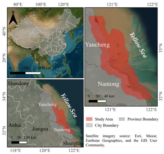
Figure 1.
Location map of the study area.
The study area is located in the eastern part of China, adjacent to the Yellow Sea, and involves the coastal areas of Yancheng City and Nantong City. This region has the largest area and the most concentrated distribution of tidal flats on the edge of the Asian continent, where the main salt marshes consist of Spartina alterniflora, Phragmites australis, and Suaeda salsa. The complex land–sea interactions in the coastal zone create significant research challenges. Due to frequent water level fluctuations caused by tidal cycles, accurately extracting information on the maximum exposed extent of land cover, especially in intertidal zones, is particularly difficult. In addition, Jiangsu coastal wetlands exhibit high local heterogeneity, characterized by fragmented patches and mixed land cover types, which manifests as spectral similarity and spatial overlap between natural and artificial water bodies, as well as among various vegetation types of salt marshes. This complexity in the classification process further exacerbates the difficulty of achieving fine-grained classification. The ecosystem characteristics and classification challenges of the study area are typically representative of coastal wetlands worldwide, and the achievements in optimizing and validating classification methods can provide important methodological references and technical support for detailed wetland classification in similar regions.
2.2. Data Source
2.2.1. Sentinel Data and Pre-Processing
A total of 215 Sentinel-1 Ground Range Detected (GRD) images and 238 Sentinel-2 surface reflectance (SR) images (date: 1 January 2020 to 31 December 2020) were selected from the GEE platform to capture temporal dynamics and spectral heterogeneity features required for wetland classification of the study area (Table 1). This specific time period was chosen because it aligns with the timeline of our ground surveys, which provided essential validation data for the classification process.

Table 1.
Satellite remote sensing data.
The Sentinel-1 imagery, consisting of vertical-vertical (VV) and vertical-horizontal (VH) polarization bands with 10 m spatial resolution, has been pre-processed based on the Sentinel-1 Toolbox, which ensures that the images are well-calibrated and adjusted to reduce noise [49]. On the other hand, the Sentinel-2 satellite is equipped with the Multi-Spectral Instrument (MSI), which supports us in obtaining visible, near-infrared (NIR), red edge, and short-wave infrared (SWIR) bands. We selected images with cloud coverage of less than 30% and masked low-quality observations caused by clouds according to the Quality Assessment (QA) 60-bitmask band [50]. In the study, six optical bands unified to 10 m spatial resolution, including Blue (B2), Green (B3), Red (B4), NIR (B8), Red Edge (B8A), and SWIR1 (B11) bands, were used for wetland mapping. Furthermore, five widely used spectral indices (Table 2) in wetland mapping that are closely related to key elements such as water, vegetation, and soil moisture [7,8,51,52]: EVI, NDVI, LSWI, NDWI and MNDWI, were calculated and inserted as bands into the initial optical and SAR images to form a high-quality dense time-series image collection.
Table 2.
Calculation of spectral indices.
2.2.2. Training and Validation Samples
From 2020 to 2021, we conducted a series of ground surveys using an unmanned aerial vehicle (UAV platform: DJI Phantom 4 Multispectral; manufacturer: DJI (Shenzhen DJI Innovation Technology Co., Ltd.), Shenzhen, China) and its built-in RGB sensors to capture submeter resolution imagery of the coastal wetlands during low tide, serving as training samples and visual interpretation references for the study. To demonstrate the level of precision in classification, we divided wetland types of the study area into three major categories, including natural wetland, artificial wetland and non-wetland, which are then further subdivided into ten subcategories (Table 3). A total of 4518 georeferenced points were collected as samples by referring to multiple sources, including existing wetland thematic collections (see Section 2.2.3), S1 and S2 lowest tide composite images (Figure 3), high-resolution Google Earth images (https://earth.google.com/ (accessed on 1 November 2025)) and UAV images. All wetland samples were randomly divided into training and testing sets with a ratio of 7:3, respectively, used for the construction of the classifier and the performance evaluation of the classifier based on ten-fold cross-validation (see Section 2.3.2).
Table 3.
Coastal wetland classification system and corresponding ground truth samples for training in the study.
As shown in Figure 2, given the significant spectral similarity and spatial overlap among the three typical salt marsh vegetation types, including Spartina alterniflora, Phragmites australis, and Suaeda salsa, we further divided salt marshes into these subcategories to validate the classification model’s ability to separate similar vegetation types, which is also one of the key challenges addressed in the study. Similarly, due to differences in exposure cycles and ecological functions, mudflats were divided into intertidal and supratidal flats. Notably, the supratidal zones between the highest tide level and artificial shorelines are often overlooked in many studies and misclassified as bare land unrelated to wetlands due to their similar spectral characteristics.
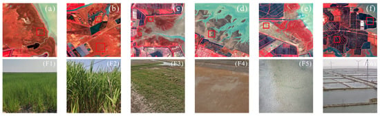
Figure 2.
Satellite images interpretation of (a) Spartina alterniflora; (b) Phragmites australis; (c) Suaeda salsa; (d) intertidal flat; (e) supratidal flat; and (f) artificial wetlands shown in color-infrared (CIR) composite Sentinel-2 image (NIR/Green/Red). Field photos of (F1) Spartina alterniflora, (F2) Phragmites australis, (F3) Suaeda salsa, (F4) intertidal flat, (F5) supratidal flat, and (F6) artificial wetlands.
Notably, coastal wetlands exhibit high dynamism, particularly in intertidal zones, where the exposed area fluctuates with tidal changes, and satellite remote sensing images often struggle to capture wetland information at the lowest and highest tidal moments [29]. To address this issue, we employed two complementary methods to ensure the accuracy and completeness of wetland information acquisition. On one hand, we used hourly tidal data for the entire year (http://mds.nmdis.org.cn/pages/tidalCurrent.html (accessed on 1 November 2025)), and identified observable optical (Figure 3a,e) and radar (Figure 3c,g) images corresponding to high and low tides within the year by linearly interpolating the hourly tidal data to seconds and assigning it to Sentinel-1/2 images that meet the screening criteria. On the other hand, we combined annual maximum composites of MNDWI and NDVI (Figure 3b,f) and quantile composites of radar data (Figure 3d,h) to extract images representing the maximum and minimum water extents, reflecting the highest and lowest tidal states (see Section 2.3.1).

Figure 3.
Sampling of intertidal wetland types with the assistance of time-series tide level data, taking Jianggang tide station as an example. (a) S2 highest tide level image observed, 31 August 2020 10:48:40 a.m., with a tide height of 515.82 cm; (b) annual maximum MNDWI composite image; (c) S1 highest tide level image observed (VH), 27 September 2020 9:55:23 a.m., with a tide height of 489.54 cm; (d) 5% composite image of annual VH; (e) S2 lowest tide level image observed, 28 April 2020 10:48:31 a.m., with a tide height of 97.34 cm; (f) annual maximum NDVI composite image; (g) S1 lowest tide level image observed (VV), 24 February 2020 9:55:13 a.m., with a tide height of 86.96 cm; (h) 95% composite image of annual VV. Abbreviations used are: S2, Sentinel-2; S1, Sentinel-1.

Based on the observable low-tide moments and their corresponding optical and SAR imagery, this study selected 50 tidal flat edge points from the observed images (Figure 3e,g). These points were systematically validated against synthetically generated low-tide optical and SAR composites. By comparing the spatial consistency of tidal flat boundaries between the observed low-tide images and their synthetic composites (Table 4), the reliability of the synthetic method in characterizing the lowest tidal conditions was verified. The integration of observed low-tide imagery with synthesized composites effectively reduces misclassification and omission errors caused by insufficient tidal sampling [53], thereby contributing to enhanced classification accuracy of wetlands in intertidal zones.
Table 4.
Consistency assessment of tidal flat boundary identification based on edge-point validation for optical and SAR imagery.
2.2.3. Ancillary Data
The digital elevation model (DEM) with 30 m resolution is derived from the Shuttle Radar Topography Mission (SRTM) and is used to extract topographic features (GEE Collection: “USGS/SRTMGL1_003”), such as elevation, slope, and aspect. The shoreline data is sourced from the full-resolution Level-1 GSHHG dataset v2.3.7, which is used for delineating the research scope and calculating the offshore distance of pixels. The data for the 6 m isobath offshore is obtained from the global relief model ETOPO 2022, which is used to edit the boundaries of the study area. Additionally, four wetland thematic datasets were used as ancillary datasets for sample collection and comparison of classification results. These include ESA_WorldCover 2020 v100, EA_Wetlands, MTWM (Multi-class Tidal Wetland Mapping), and CMSA (China mainland Spartina alterniflora). The ESA_WorldCover 2020 v100 dataset is a global land cover map produced by the European Space Agency (ESA) with Sentinel-1/2 imagery [54]. The EA_Wetlands product in 2021 is a 10 m wetland map of East Asia, integrating object-based and decision-tree classification methods [55]. The MTWM product in 2020 is a 10 m tidal wetlands map of East Asia, generated by using tidal level and phenological features [20]. The CMSA product (2017–2021) provides 10 m spatial distribution maps of Spartina alterniflora in China using DeepLabv3+ with temporal transfer learning [56]. The specific sources of the ancillary data are shown in Table 5.
Table 5.
Sources and applications of auxiliary data.
2.3. Technical Framework for Wetland Classification and Analysis
A hierarchical, detailed classification strategy for coastal wetlands is proposed, as shown in Figure 4. Firstly, based on the constructed Sentinel-1/2 image data stack, a set of feature variables, including water level features, phenological features, variation features, geographic features, and topographic features, was established to capture information on periodically submerged and poorly distinguishable coastal wetland features, combined with multi-source data such as tidal levels, shorelines, and DEM. Secondly, a preliminary classification of coastal wetlands was conducted using a pixel-based random forest classification method. Then, an object-based random forest classification method was applied to distinguish between natural and artificial water bodies using various shape features. The final classification results were obtained by integrating classification results from the pixel-based and object-based stages through post-processing. Thirdly, the pixel-based and object-based classification results are merged. Specifically, the detailed water body types derived from the object-based classification are overlaid onto the preliminary pixel-based classification results, enabling fine-grained mapping of the Jiangsu coastal wetlands. Furthermore, the accuracy of the results is evaluated, and comparisons are made with published wetland products in terms of area and distribution to validate the feasibility of the proposed model and the reliability of the classification results.
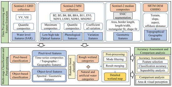
Figure 4.
The framework for the classification of coastal wetlands and analysis.
2.3.1. Feature Extraction of Coastal Wetlands
Based on the GEE platform, we computed multi-source feature variables required for pixel-based and object-based wetland classification, respectively (Table 6 and Table 7). The pixel-based wetland classification features include 22 optical water level features, 55 percentile-composited phenological features, 11 coefficients of variation features, 4 SAR water level features, 3 topographic features, and 1 geographic feature. The object-based wetland classification features include 2 optical features and 5 shape features.
Table 6.
Pixel-based features variables adopted for wetland classification.
Table 7.
Object-based features variables adopted for wetland classification.
The observable characteristics of coastal wetlands change rapidly with daily water levels. To capture wetland information in both fully submerged and maximally exposed states, the qualityMosaic() function was used to calculate annual maximum values of MNDWI and NDVI for each pixel within the time series, generating composites that characterize extreme tidal conditions to represent the maximum and minimum water extents (Figure 3b,f) [53,57]. Additionally, band information from the maximum composites index was integrated to comprehensively monitor the differences in wetlands under various hydrological conditions. Given that optical observations are often affected by the weather, and considering that SAR supports all-weather observations and is sensitive to soil moisture, water bodies, and vegetation structure [58], SAR time-series data were also used as an additional supplement to capture the highest and lowest water level composites. Specifically, to mitigate potential residual noise and interference, the percentile() function was used to compute the 5th percentile of Sentinel-1 VV and VH for synthesizing the highest water level information, while the 95th percentile of VV and VH was used to synthesize the lowest water level information (Figure 3d,h) [53].
To address seasonal variations and spectral similarity among coastal wetland types, percentile composites (10th, 25th, 50th, 75th, and 90th) of each band and index were calculated to extract phenological features. Compared to traditional methods that rely on identifying key phenological stages, the percentile-based approach achieves similar mapping accuracy without the need for prior knowledge [59] and applies to large-scale applications without region-specific adjustments [60]. Figure 5a shows the annual phenological curves of three typical salt marshes, derived from Savitzky–Golay filtered NDVI observations. Based on these curves, the inference of phenological stages for different salt marshes is relatively complex and exhibits certain regional variations. In comparison, percentile-based features effectively capture seasonal and developmental phase differences while significantly reducing the manual effort and potential errors associated with conventional phenological interpretation (Figure 5b).
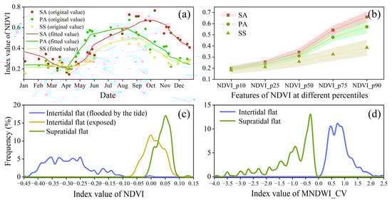
Figure 5.
Display of several key features for distinguishing subcategories of salt marshes and mudflats in the study. Note: Spartina alterniflora (SA), Phragmites australis (PA), Suaeda salsa (SS). (a) The annual fitted NDVI curves of three typical salt marshes; (b) comparison of annual NDVI percentile features among three typical salt marshes; (c) frequency comparison of NDVI index between supratidal and intertidal flats (exposed or flooded); (d) frequency comparison of MNDWI_CV index between supratidal and intertidal flats.
Additionally, the Coefficient of Variation (CV) was employed to quantify temporal variability in coastal wetlands [61]. Calculated as the ratio of standard deviation to mean of indices, CV effectively captures the frequent periodic inundation characteristic of intertidal areas. While supratidal and intertidal flats exhibit similar spectral characteristics in composite imagery, with intertidal zones showing only slightly higher moisture content (Figure 5c), CV analysis quantitatively measures differences in tidal inundation frequency, enabling clear separation between supratidal and intertidal flats (Figure 5d).
Due to the similarity in physical characteristics (e.g., watercolor and inundation frequency) between coastal artificial wetlands and natural water bodies, it is difficult to distinguish them relying solely on pixel-based features. The Simple Non-Iterative Clustering (SNIC) method was applied to the annual median Sentinel-2 composites to obtain superpixel segmentation results [62]. Subsequently, shape features for each object were calculated, including area, border length, length-to-width ratio, rectangular fit, and shape index (Table 7). Benefiting from the fact that artificial wetlands have more regular shapes and boundary features, these features can better distinguish the natural/artificial attributes of water bodies.
In addition, topographic features such as elevation, slope, and aspect, as well as geographic features like distance to the shoreline, were incorporated as auxiliary features to assist in coastal wetland classification. Generally, wetland formation is more likely in areas with flatter, lower-lying terrain and closer proximity to the coastline.
2.3.2. Random Forest Classifier
Random forest classifier is an ensemble learning method that works by constructing multiple decision trees and aggregating their prediction results [63]. While increasing the number of trees typically enhances model performance, it also demands greater computational resources. Therefore, it is essential to determine the appropriate number of decision trees based on specific task requirements to achieve an optimal balance between classification accuracy and computational efficiency. Compared to other supervised machine learning algorithms, the random forest algorithm demonstrates significant advantages in terms of training efficiency and capability in handling high-dimensional data, making it widely applicable to robust wetland classification under complex environmental conditions with numerous feature inputs [40,52,64]. Moreover, the algorithm can utilize an out-of-bag error evaluation mechanism to automatically quantify the contribution of each feature to the classification results, thereby providing a reliable basis for feature selection [62]. In this study, the Random Forest algorithm was implemented using the ee.Classifier.smileRandomForest() function on the GEE platform.
2.3.3. Pixel-Based Classification
There are 96 multi-source feature variables used in pixel-based classification, excluding shape features, to perform pixel-by-pixel classification based on the random forest algorithm, yielding preliminary classification results. The results included 9 categories: Spartina alterniflora, Phragmites australis, Suaeda salsa, intertidal flat, supratidal flat, water bodies, built-up land, forest land, and cropland. To balance algorithm efficiency and classification accuracy, the number of decision trees in the random forest model was set to 200 in GEE, while other parameters remained at their default values.
Although the extensive feature variables selected could sufficiently reflect the intrinsic characteristics of wetlands, they also resulted in high model complexity and redundancy. To address this, RFE was employed to screen and eliminate redundant features [65,66]. The out-of-bag error from the random forest algorithm was employed to evaluate the relative importance of feature variables and rank them accordingly. The RFE process initiated with all candidate features and iteratively eliminated the least important feature based on importance scores at each step, continuing until only one feature remained, thereby generating a series of feature subsets. For each subset, twenty rounds of ten-fold cross-validation were performed by the random forest model to identify the optimal feature subset with the highest average accuracy for the classification model, ensuring the model maintained high accuracy while achieving faster computational performance.
2.3.4. Object-Based Classification
Object-based classification is used to distinguish the natural or artificial attributes of water bodies, categorizing them into two subclasses: permanent water and artificial wetland. The SNIC algorithm was applied in GEE to segment the annual median composite Sentinel-2 imagery. SNIC can group neighboring pixels into clusters effectively in a bottom-up, seed-based manner [67]. Its segmentation performance primarily depends on three key parameters: superpixel seed location spacing (controlling superpixel size and quantity), compactness (balancing spatial proximity with spectral similarity), and connectivity (defining pixel adjacency relationships). To ensure that the segmented image objects are closely aligned with the target features, the parameters of the SNIC model were optimized through iterative testing and validation: superpixel seed location spacing was set to 16 pixels, compactness to 0.5, and connectivity to 8. Based on the segmentation results, seven features were extracted for each object, including shape features and the mean values of NDVI and MNDWI. A random forest model with 100 decision trees and default parameters was then constructed to classify the objects into three categories: non-water, permanent water, and artificial wetland.
2.3.5. Post Classification Processing
The pixel-based and object-based classification results were integrated through a hierarchical fusion strategy to ensure the accuracy and spatial consistency of the final wetland map. Specifically, the permanent water and artificial wetlands identified in the object-based classification results were overlaid onto the water bodies extracted from the pixel-based classification results, enabling the complementary advantages of both methods: the pixel-based classification preserves fine spatial details of land cover, while the object-based classification refines the functional attributes within water bodies. For non-overlapping regions with conflicting labels, the pixel-based results were primarily retained, supplemented by visual interpretation for relabeling. To reduce noise caused by pixel-based classification, a 3 × 3 majority filter with an 8-connected neighborhood kernel was applied to determine category attribution judgment, which significantly improved the regional homogeneity while maintaining boundary clarity.
2.4. Jeffries–Matusita Distance
In the preliminary pixel-based classification, we conducted feature selection from the extensive feature variable set. To ensure the representativeness of the selected feature combination, the Jeffries–Matusita (JM) distance was employed to analyze the separability of typical land cover types. The JM distance, calculated based on features, measures the distance between samples of different classes and serves as an effective tool for evaluating inter-class separability. It can be expressed by (6) and (7) [68].
Here, B represents the Bhattacharyya distance in a specific feature dimension; denotes the mean of a feature for a given class; represents the variance of a feature for a given class, where k = 1, 2. The JM distance involves values between 0 and 2, representing the separability between samples of different classes. The closer the value is to 2, the higher the degree of separation between the two land cover types under the selected classification features. Conversely, the closer the value is to 0, the lower the degree of separation. Generally, if the value of the JM distance exceeds 1.8, it indicates a good degree of separability between different samples.
2.5. Accuracy Assessment and Comparison Analysis
To validate the reliability of the classification results, a combination of qualitative visual comparison and quantitative metrics was employed. On the one hand, the study collected four existing datasets that have proven to be effective within the scope of the study area, involving various land cover datasets and wetland thematic datasets (see Table 5), which were used to compare the consistency of the area and distribution with the classification results. On the other hand, a stratified random sampling scheme was adopted to collect validation samples that were spatially independent of the training samples, effectively preventing the inflation of accuracy estimates due to spatial autocorrelation and ensuring a rigorous assessment of the model’s generalization capability. We calculated that 3318 samples were needed for validation according to the commonly used sample size formula [69], as shown below:
where = 1.96 for a 95% confidence interval, is the half-width of the desired confidence interval ( = 0.05 in this study), is the anticipated proportion of correct classifications for a particular class. Since the characteristics of water bodies are significantly different from those of other land types, a better classification effect is expected. We set of water bodies to 0.8 and calculated that 246 samples were required. For the other land types, we set as 0.5 to obtain a large enough value (the term p(1 − p) is maximized at this value) due to the lack of knowledge on the correct anticipated proportion of the other classes. It is calculated that 384 samples are, respectively, required for each of the other classes. As a result, we acquired a sample validation set and randomly and evenly distributed these sample points by quantity across each category for validation purposes. Accuracy evaluation metrics, including overall accuracy (O.A.), kappa coefficient, user’s accuracy (U.A.), producer’s accuracy (P.A.), and F1 score, were calculated based on the confusion matrix to assess the model’s accuracy.
3. Results
3.1. Feature Selection Analysis
In the object-based classification, since water bodies and non-water bodies can be clearly distinguished using NDVI and MNDWI, and artificial wetlands are easily differentiated from permanent water due to their regular shapes, a typical and moderate number of features was only required to meet the classification requirements. In contrast, in the pixel-based classification, an excessive number of redundant features were used. So, to balance model efficiency and accuracy, feature selection was crucial.
The 96 features, excluding shape features, were divided into six main feature types: optical water level features, phenological features, variation features, SAR features, topographic features, and geographic features. Figure 6 illustrates the relationship between the number of features selected using RFE and the accuracy of ten-fold cross-validation, and the confidence bands at the 95% confidence level were calculated to evaluate the uncertainty of the cross-validation results. Features were sequentially input into the classifier in ascending order of their importance. It can be observed that when the number of input features was small, the training accuracy increased rapidly with the addition of features. However, when the number of features exceeded 26, the improvement in training accuracy gradually leveled off, fluctuating between 0.88 and 0.90. When the number of input features reached 71, the model achieved the highest cross-validation accuracy of 0.901, indicating that this feature combination represents the optimal set after feature screening. Adding more features beyond this point would not only introduce unnecessary redundancy into the model but also result in a decline in classification accuracy. Ultimately, approximately one-third of the original features were removed through the screening process. The retained features included 17 optical water level features, 43 phenological features, 6 variation features, 4 SAR features, and 1 distance-to-shore feature.
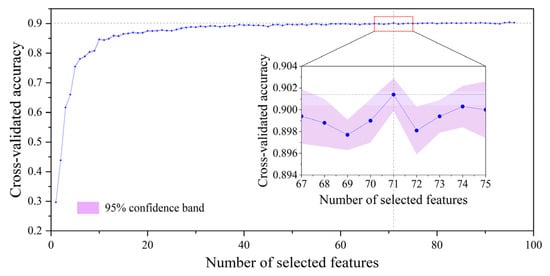
Figure 6.
The relationship between the number of features and cross-validated accuracy.
Figure 7 illustrates the relative importance of retained features as determined by the random forest algorithm, with features sorted by their respective types to highlight the contribution of each feature to the classification. Among them, phenological features and SAR features contributed the greatest, benefiting from the full utilization of vegetation phenology and water level dynamics. Optical water level features and variation features followed as they were more effective in extracting water-sensitive wetlands, such as intertidal flats and periodically submerged salt marshes. Offshore distance was also comparatively important, as areas closer to the coast are more likely to be wetlands due to higher moisture levels. In contrast, topographic features demonstrated relatively lower discriminative power and were consequently eliminated during the feature selection, despite being initially included to ensure a comprehensive evaluation of all potentially relevant variables. Although wetland formation is generally associated with terrain variations and typically occurs in low-lying areas, the predominantly flat topography of the study area limited the statistical relevance of these features for classification in this particular environment.
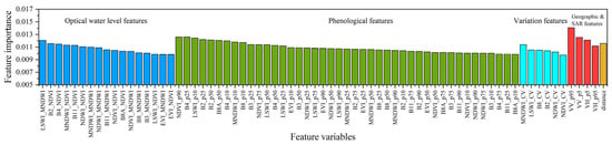
Figure 7.
The relative importance of features. Note: explanations of feature names can be found in Table 6. Suffixes in feature names such as “_NDVI” or “_MNDWI” denote features that are based on the maximum composites of NDVI or MNDWI. Suffixes like p25 and p95 refer to percentile values. The suffix “_CV” represents the coefficient of variation for each band.
After feature selection, the five most representative features with the highest importance scores from each of the five feature types were chosen to create boxplots, analyzing the separability performance of different land cover types under these optimal features. As shown in Figure 8, LSWI_MNDWI, derived from the highest water level composite imagery, effectively distinguishes water bodies and intertidal flats from other land cover types. Furthermore, NDVI_p90 and VV_p95, representing the low water level composite imagery, along with MNDWI_CV, which captures dynamic changes, enable the differentiation between permanently covered water bodies and periodically exposed intertidal flats. Due to the sparse distribution of Suaeda salsa, NDVI_p90 can separate it from denser vegetation types such as Spartina alterniflora, Phragmites australis, cropland, and forest land. Moreover, the distance feature helps identify the vegetation gradient from the coastline inland, revealing a distribution pattern of Spartina alterniflora—Suaeda salsa—Phragmites australis, which aligns with field survey results.
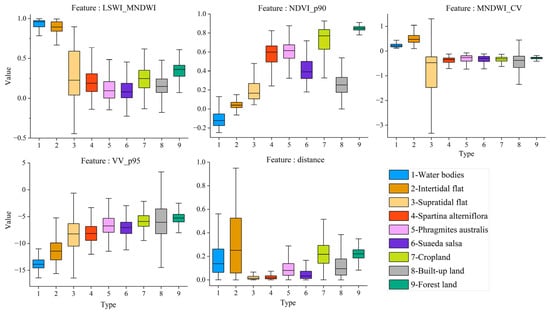
Figure 8.
Box plots corresponding to the five most important features among the five types of features.
3.2. Detailed Classification Results of Coastal Wetland Types
As shown in Figure 9, based on the proposed classification model and multi-source remote sensing data, the overall classification results of the study area were produced with 7 wetland types and 3 non-wetland types. From the perspective of overall visual interpretation, artificial wetlands and salt marshes are primarily distributed in the transitional zones from the coast to the inland, with a concentrated presence in the coastal areas of Yancheng. In contrast, artificial wetlands in Nantong are more fragmented and scattered. Inland areas are predominantly characterized by farmland and construction land. To further evaluate the classification effectiveness, five representative regions were selected (see Figure 9, Sites A–E), each highlighting distinct wetland characteristics and mapping challenges, providing a comprehensive assessment of the model’s performance across diverse geographical and ecological contexts. Figure 9a, corresponding to Site A, demonstrates the capability of the classification model to distinguish three typical types of coastal salt marsh vegetation. By leveraging the offshore distance and phenological features, the model effectively addresses the issue of spectral similarity among different salt marshes. Figure 9b, corresponding to Site B, uses Sentinel-2 high-tide imagery to illustrate the extraction of supratidal flats between high-tide water levels and artificial shorelines. Similarly, Figure 9c–e utilize Sentinel-2 low-tide imagery to detail the extraction of intertidal flats in different geographical locations, such as near-shore areas and estuaries, with accurate identification of their boundaries and extents. Additionally, Figure 9b,e also highlight the model’s ability to distinguish between permanent water and artificial wetlands in adjacent or connected water bodies.
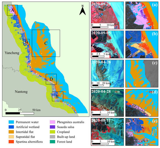
Figure 9.
The wetland mapping results of the study area. Note: Five typical regions (Sites A–E) were selected to demonstrate the classification effectiveness. Site A (the core area of Yancheng Wetland National Nature Reserve); Site B (the estuary of Chuandong Port); Site C (intertidal flats in Dongtai District); Site D (Yangkou Port); Site E (Tongzhou Bay). (a–e) show the wetland mapping results corresponding to Sites A–E in sequence, respectively.
The ee.Reducer.sum() function was used based on GEE to count the number of pixels of various land types in the classification results and conduct a summary calculation of the area. The area statistics of wetlands and non-wetlands are provided in Table 8. The coastal wetlands area of the study area in 2020 was 8894.14 km2, including 8346.71 km2 of natural wetlands and 547.43 km2 of artificial wetlands. Salt marshes, mudflats, permanent water, and artificial wetland accounted for 6.71%, 31.22%, 55.92% and 6.15% of the total coastal wetland area, respectively. Among individual wetland types, permanent water had the largest area, followed by intertidal flats, artificial wetlands, Phragmites australis, Spartina alterniflora, supratidal flats, and Suaeda salsa. Among non-wetland types, cropland had the largest area, followed by built-up land and forestland.
Table 8.
Area statistics of wetlands and non-wetlands in the study area.
3.3. Accuracy Assessment of Coastal Wetland Classification Results
The accuracy of the classification results was quantitatively evaluated using validation samples. For the pixel-based classification results, the overall accuracy reached 92.50%, with a kappa coefficient of 0.915. Figure 10 further displays the producer’s accuracy, user’s accuracy, and F1 score for different land cover types. Among wetland types, most wetlands achieved U.A., P.A., and F1 scores above 0.900, except for Suaeda salsa. For non-wetland types, built-up land, forest land, and cropland exhibited high accuracy, with F1 scores of 0.946, 0.943, and 0.928, respectively. Specifically, water bodies and intertidal flats showed excellent separability from other land cover types, with U.A., P.A., and F1 scores all exceeding 0.950. This is primarily due to the unique and stable spectral characteristics of water bodies, as well as the inclusion of water level and variation features, which distinguish the periodically submerged characteristics of intertidal flats from other land cover types. In contrast, supratidal flats had relatively lower classification accuracy, with an F1 score of 0.898, due to confusion with intertidal flats and unused built-up land. Among the three main salt marsh types, Spartina alterniflora achieved the highest classification accuracy, followed by Phragmites australis and Suaeda salsa. The sparse and scattered distribution of Suaeda salsa often led to omission errors, resulting in an F1 score below 0.888. Although Phragmites australis performed well in classification, they were occasionally confused with cropland.
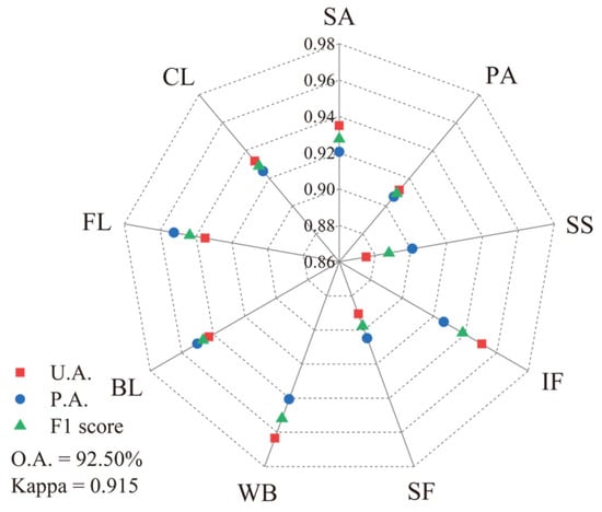
Figure 10.
Accuracy assessment of pixel-based classification. Note: Spartina alterniflora (SA), Phragmites australis (PA), Suaeda salsa (SS), intertidal flat (IF), supratidal flat (SF), water bodies (WB), built-up land (BL), forest land (FL) and cropland (CL).
For the object-based classification results of water bodies, Table 9 presents the confusion matrix for permanent water and artificial wetlands, including U.A., P.A., and F1 scores. Both categories achieved F1 scores above 0.920, indicating excellent separability. This can be attributed to the more regular shapes or boundary features of artificial wetlands, which clearly distinguish them from natural permanent water.
Table 9.
Confusion matrix of object-based classification. Note: permanent water (PW) and artificial wetland (AW).
4. Discussion
4.1. Separability Analysis of Coastal Wetland Types
To verify the effectiveness of the feature variable combinations screened by RFE in distinguishing different wetland types, the separability between them was analyzed using the JM distance, thereby providing important reference information for the model’s classification performance [39]. The separability between different wetland types is shown in Table 10. The separability among the nine wetland types is fine, with JM distances all greater than 1.96, fully meeting the requirements of the actual study. Among them, intertidal flats, water bodies, and forest land all have high separability from other wetland types, indicating that these wetland types are relatively independent in the feature space and easy to distinguish. This is consistent with the conclusions in the accuracy validation section (see Section 3.3). Due to the sparse distribution of Suaeda salsa on the supratidal flats or the pond ridges connected to aquaculture ponds, and the similar spectral characteristics between the supratidal flats and the unused bare land of built-up land, the separability of the supratidal flats from the two is relatively low [70]. Additionally, the analysis of JM distances among the three types of typical coastal salt marsh reveals inevitable misclassification due to their spatial distribution and spectral similarity [71], particularly between Spartina alterniflora and Phragmites australis. It is also noteworthy that Phragmites australis are often distributed along riverbanks and irrigation channels, closely adjacent to cropland in the landscape, and share similar vegetation structures and spectral characteristics. Consequently, the separability between cropland and Phragmites australis is relatively low compared to other vegetation types.
Table 10.
Separability evaluation based on JM distance between different wetland types.
4.2. Comparison with Other Dataset Products
To validate the reliability of the proposed model, the classification results were compared with four existing datasets in terms of area and spatial distribution for major wetland types, including tidal flats, salt marshes, Spartina alterniflora, and artificial wetlands, within the same regions. Table 11 presents the estimated areas of major wetland types from different studies. It can be observed that the tidal flat area estimates in this study align closely with those from MTWM, showing a 96.49% spatial overlap. This high consistency is likely attributed to the representation of tidal cyclic inundation characteristics and the application of similar sampling strategies specific to tidal flats [20], which EA_Wetlands overlooked. Similarly, the artificial wetland area estimates in this study are consistent with those from EA_Wetlands, as both studies employed object-based strategies and utilized shape features to distinguish natural and artificial water bodies. For Spartina alterniflora, the similar area estimates between this study and CMSA, with a spatial consistency accounting for 75.80%, may result from both strategies’ thorough consideration of spectral-phenological features [56], which effectively enhanced the separability between Spartina alterniflora and other coexisting vegetation species. In comparison with multiple datasets, significant variations in salt marsh area estimates were noted. However, this does not directly imply inaccuracies in the results of this study. The differences in research scope and classification strategies have led to divergent results. The MTWM was limited to intertidal zones and did not cover salt marshes in supratidal areas, resulting in an underestimation of total salt marsh area. ESA_WorldCover performed poorly in identifying salt marshes, often misclassifying them as cropland or water bodies, which aligns with findings from similar studies [13]. Compared to MTWM and this study, EA_Wetlands exhibited omission errors in the classification of salt marshes, which were further confirmed through field surveys. This is mainly because EA_Wetlands only adopted an object-oriented classification strategy [55], and the object segmentation process ignored small and micro salt marsh wetlands, resulting in their failure to be effectively identified and classified.
Table 11.
Comparison between classification results and other datasets in a wetland-type area.
Figure 11 illustrates the spatial distribution comparison of coastal wetland types between the results of the study and other datasets. To minimize discrepancies arising from interannual variations, regions with low interannual dynamics were selected for comparison. Although MTWM focused solely on intertidal zones, the distribution of tidal flats and salt marshes in these areas shows high consistency with the results of the study, as both approaches integrated water level features and phenological features (Figure 11a–d). The ESA_WorldCover dataset, designed for global coverage, lacks detailed classification systems at the regional level and does not specifically account for tidal flat categories [54]. Despite this limitation, its water body distribution aligns well with the results of the study. In addition, ESA_Worldcover also provides the distribution of non-wetland types, which can be used to compare the misclassification of different wetland types in various existing wetland thematic datasets. For example, there is the missed classification of supratidal flats and the misclassification between them and bare land (Figure 11c), as well as the misclassification between cropland and salt marshes (e.g., Phragmites australis) (Figure 11a,d), etc. These misclassification instances also align with the separability assessment results presented in Section 3.1. EA_Wetlands, which only employed an object-based classification approach, achieved more efficient image analysis. Nevertheless, comparisons reveal that EA_Wetlands overlooks many internal details of objects and provides an incomplete extraction of tidal flat categories. For instance, in Figure 11c, the permanently exposed supratidal flats were not classified as wetlands, and roads and vegetation separating water bodies were also omitted, leading to insufficient detail due to the lack of pixel-level features. Additionally, while the Spartina alterniflora distribution mapped by CMSA shows high consistency with this study in supratidal zones (Figure 11a–c), it exhibits partial omissions in intertidal zones (Figure 11d). The omissions occurred because the labeled samples input to its DeepLabv3+ model were derived from median composite images after cloud and water masking [56], without fully accounting for tidal fluctuations that characterize dynamic coastal wetlands, consequently missing submerged Spartina alterniflora patches in intertidal zones. Overall, compared to existing datasets, the proposed method effectively captures the intrinsic differences in land cover in highly dynamic and heterogeneous coastal wetland environments at both pixel and object levels, while maintaining superior accuracy and computational efficiency in extracting key wetland types such as tidal flats, artificial wetlands, and salt marshes during multi-classification tasks.
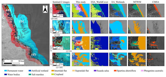
Figure 11.
Comparison between research results and other datasets in wetland-type distribution. Note: Four typical regions (a–d) were selected to compare the classification results of this study with other datasets. (a) Yancheng Wetland National Nature Reserve; (b) intertidal zones in Dongtai District; (c) Fangtang Estuary; (d) Tongzhou Bay.
4.3. Limitations and Improvement
Through accuracy validation and comparative experiments, the coastal wetland classification strategy proposed in the study has been proven to achieve high accuracy, with classification results demonstrating relatively superior visual interpretability. However, influenced by various factors such as input image data, classification algorithms, wetland classification systems, and sample accuracy, there remain certain uncertainties and limitations. First, in the study, high-quality observations from Sentinel-1/2 in 2020 were selected, and most low-quality observations affected by clouds were removed using QA bands to ensure as much high-quality data as possible for each pixel to meet the requirements of the classification model. Nevertheless, spatial inconsistencies in the number of high-quality observations per pixel objectively persist [64], causing uncertainties that not only compromise the integrity of time-series analysis but also lead to spatial heterogeneity in critical features, such as phenological features and variation features, consequently reducing the reliability of pixel-level classification results. Meanwhile, due to the uncertainty of local instantaneous tidal conditions during the satellite overpassing, the number of images acquired during low tide periods throughout the year is considerably limited [20,53]. Particularly in intertidal zones, although this study synthesizes images from temporal statistical values of optical and SAR features to simulate the distribution of ground objects at the maximum exposure during low tide, the limitation of observation windows still fails to ensure an adequate number of non-inundated exposed pixels, posing challenges for precise land cover classification. To further mitigate the impacts of cloud contamination and tidal variations on data quality, future work could explore the application of spatiotemporal fusion algorithms to integrate multi-source remote sensing data with varying spatial and temporal resolutions, generating denser high-quality image observations [72,73]. Second, the high dynamism of coastal wetlands, combined with their low intra-class homogeneity and high inter-class heterogeneity, amplifies the uncertainties in sample interpretation. Particularly under the fine classification system, the collection of samples for spatially overlapping and spectrally similar features, such as typical salt marshes and supratidal/intertidal flats, often leads to additional subjective labeling errors and workload. While existing wetland thematic datasets enable the automatic and rapid collection of large amounts of training samples [74,75], discrepancies exist among these datasets in terms of spatial resolution, spatiotemporal coverage and classification systems, and the datasets themselves also contain errors. These factors limit the accuracy of dataset-based automatic sample labeling methods and make it difficult to apply such methods to the sample collection of small-scale, specific wetland types lacking reference products, such as Suede salsa and supratidal flats. Future research could focus on sample transfer and expansion to address this challenge [76]. Third, the geographical scope and temporal span of the study are limited. While focusing on typical coastal wetlands in Jiangsu, it should be recognized that environmental differences across regions, including hydrological conditions (e.g., tidal patterns and water turbidity), topographic features, and vegetation composition (e.g., herbaceous and woody marshes), may cause differences in feature sensitivity and model performance when applying the method. Future efforts should extend the proposed method to multiple regions with diverse tidal patterns and vegetation communities, as well as to longer temporal scales [9], in order to systematically evaluate its transferability and robustness across a wider range of coastal wetland ecosystems. Fourth, our classification algorithm may have overestimated the area of salt marshes, particularly for Phragmites australis and Suaeda salsa. This overestimation is mostly due to the spectral similarity between Phragmites australis and croplands, which creates uncertainty in sample interpretation and subsequent misclassification. Additionally, the scattered distribution and small patch sizes of Suaeda salsa contribute to lower extraction accuracy. These findings suggest the need for further targeted validation and refinement of the algorithm’s performance for specific salt marsh vegetation types. Fifth, future research could explore integrating deep learning classifiers with the dynamic differential features of coastal wetlands extracted in this study as attention mechanism inputs, which may further enhance the generalization capability and efficiency of the model [77,78].
5. Conclusions
This study developed a pixel- and object-based hierarchical classification strategy to address challenges of tidal fluctuations, cloud contamination, and spectral similarity of land cover types, with its reliability in the detailed classification of typical Jiangsu coastal wetlands verified. By reconstructing high-quality Sentinel-1/2 time-series image stacks, extracting pixel-level temporal statistical features, and incorporating topographic and geographic features, this strategy captures the dynamics of water levels and the stage of vegetation phenology in coastal wetlands, significantly improving the separability and classification accuracy of wetland types. Furthermore, geometric features derived from image object segmentation are used to distinguish natural and artificial attributes of coastal water bodies, enabling fine-grained wetland mapping. The results demonstrate that the detailed wetland mapping scheme achieved an O.A. of 92.5% and a Kappa coefficient of 0.915 across 7 wetland types and 3 non-wetland types. Quantitative accuracy assessments, along with comparisons of area estimates and visual interpretations with existing datasets, indicate that the proposed strategy demonstrates reliable performance in coastal wetland areas, particularly in the identification of intertidal flats, salt marshes, and artificial wetlands. The research findings can provide technical support for ecological research and sustainable management of coastal wetlands. Applying this strategy to long-term monitoring projects of coastal wetlands in diverse environments is planned for the next step to detect its spatiotemporal universality.
Author Contributions
Conceptualization, H.X.; data curation, H.X. and J.X.; formal analysis, H.X. and S.Z.; investigation, J.X., J.W. and H.H. (Haoran Hu); methodology, H.X. and S.Z.; resources, H.H. (Huping Hou); software, H.X. and J.W.; visualization, H.X. and H.H. (Haoran Hu); writing—original draft preparation, H.X.; writing—review and editing, H.X. and S.Z.; supervision, S.Z. and H.H. (Huping Hou). All authors have read and agreed to the published version of the manuscript.
Funding
This research was funded in part by Jiangsu Provincial Natural Resources Department (Grant No. JSZRHYKJ202204 and No. JSZRKJ202422), in part by the Graduate Innovation Program of China University of Mining and Technology (Grant No. 2024WLKXJ180), and in part by the Postgraduate Research & Practice Innovation Program of Jiangsu Province (Grant No. KYCX24_2830).
Data Availability Statement
The original data that support the findings of this study are contained within the article. Further inquiries can be directed to the corresponding author.
Acknowledgments
We acknowledge ESA and Google Earth Engine platform for providing satellite imagery.
Conflicts of Interest
The authors declare no conflicts of interest.
Abbreviations
The following abbreviations are used in this manuscript:
| RFE | recursive feature elimination |
| GEE | Google Earth Engine |
| VV | vertical–vertical |
| VH | vertical–horizontal |
| NIR | near-infrared |
| SWIR | short-wave infrared |
| EVI | Enhanced Vegetation Index |
| NDVI | Normalized Difference Vegetation index |
| LSWI | Land Surface Water Index |
| NDWI | Normalized Difference Water Index |
| DEM | digital elevation model |
| CV | coefficient of variation |
| SNIC | simple non-iterative clustering |
| JM | Jeffries–Matusita |
| O.A. | overall accuracy |
| U.A. | user’s accuracy |
| P.A. | producer’s accuracy |
| PW | permanent water |
| AW | artificial wetland |
| SA | Spartina alterniflora |
| PA | Phragmites australis |
| SS | Suaeda salsa |
| IF | intertidal flat |
| SF | supratidal flat |
| WB | water bodies |
| BL | built-up land |
| FL | forest land |
| CL | cropland |
References
- Sun, Z.; Sun, W.; Tong, C.; Zeng, C.; Yu, X.; Mou, X. China’s Coastal Wetlands: Conservation History, Implementation Efforts, Existing Issues and Strategies for Future Improvement. Environ. Int. 2015, 79, 25–41. [Google Scholar] [CrossRef]
- Wang, X.; Xiao, X.; Zou, Z.; Hou, L.; Qin, Y.; Dong, J.; Doughty, R.B.; Chen, B.; Zhang, X.; Chen, Y.; et al. Mapping Coastal Wetlands of China Using Time Series Landsat Images in 2018 and Google Earth Engine. ISPRS J. Photogramm. Remote Sens. 2020, 163, 312–326. [Google Scholar] [CrossRef]
- Wang, X.; Xiao, X.; Xu, X.; Zou, Z.; Chen, B.; Qin, Y.; Zhang, X.; Dong, J.; Liu, D.; Pan, L.; et al. Rebound in China’s Coastal Wetlands Following Conservation and Restoration. Nat. Sustain. 2021, 4, 1076–1083. [Google Scholar] [CrossRef]
- He, Q.; Silliman, B.R. Climate Change, Human Impacts, and Coastal Ecosystems in the Anthropocene. Curr. Biol. 2019, 29, R1021–R1035. [Google Scholar] [CrossRef]
- Wu, W.; Zhi, C.; Gao, Y.; Chen, C.; Chen, Z.; Su, H.; Lu, W.; Tian, B. Increasing Fragmentation and Squeezing of Coastal Wetlands: Status, Drivers, and Sustainable Protection from the Perspective of Remote Sensing. Sci. Total Environ. 2022, 811, 152339. [Google Scholar] [CrossRef]
- Wei, L.; Mao, M.; Zhao, Y.; Wu, G.; Wang, H.; Li, M.; Liu, T.; Wei, Y.; Huang, S.; Huang, L.; et al. Spatio-Temporal Characteristics and Multi-Scenario Simulation Analysis of Ecosystem Service Value in Coastal Wetland: A Case Study of the Coastal Zone of Hainan Island, China. J. Environ. Manage. 2024, 368, 122199. [Google Scholar] [CrossRef] [PubMed]
- Zhang, X.; Liu, L.; Zhao, T.; Chen, X.; Lin, S.; Wang, J.; Mi, J.; Liu, W. GWL_FCS30: A Global 30 m Wetland Map with a Fine Classification System Using Multi-Sourced and Time-Series Remote Sensing Imagery in 2020. Earth Syst. Sci. Data 2023, 15, 265–293. [Google Scholar] [CrossRef]
- Mao, D.; Wang, Z.; Du, B.; Li, L.; Tian, Y.; Jia, M.; Zeng, Y.; Song, K.; Jiang, M.; Wang, Y. National Wetland Mapping in China: A New Product Resulting from Object-Based and Hierarchical Classification of Landsat 8 OLI Images. ISPRS J. Photogramm. Remote Sens. 2020, 164, 11–25. [Google Scholar] [CrossRef]
- Murray, N.J.; Worthington, T.A.; Bunting, P.; Duce, S.; Hagger, V.; Lovelock, C.E.; Lucas, R.; Saunders, M.I.; Sheaves, M.; Spalding, M.; et al. High-Resolution Mapping of Losses and Gains of Earth’s Tidal Wetlands. Science 2022, 376, 744–749. [Google Scholar] [CrossRef] [PubMed]
- Jia, M.; Wang, Z.; Mao, D.; Ren, C.; Song, K.; Zhao, C.; Wang, C.; Xiao, X.; Wang, Y. Mapping Global Distribution of Mangrove Forests at 10-m Resolution. Sci. Bull. 2023, 68, 1306–1316. [Google Scholar] [CrossRef]
- Ahmad, H.; Abdallah, M.; Jose, F.; Elzain, H.E.; Bhuyan, M.S.; Shoemaker, D.J.; Selvam, S. Evaluation and Mapping of Predicted Future Land Use Changes Using Hybrid Models in a Coastal Area. Ecol. Inform. 2023, 78, 102324. [Google Scholar] [CrossRef]
- Zheng, Z.; Jia, R. Distribution and Structure of China–ASEAN’s Intertidal Ecosystems: Insights from High-Precision, Satellite-Based Mapping. Remote Sens. 2025, 17, 155. [Google Scholar] [CrossRef]
- Li, M.; Chen, B.; Webster, C.; Gong, P.; Xu, B. The Land-Sea Interface Mapping: China’s Coastal Land Covers at 10 m for 2020. Sci. Bull. 2022, 67, 1750–1754. [Google Scholar] [CrossRef] [PubMed]
- Yang, X.; Zhu, Z.; Qiu, S.; Kroeger, K.D.; Zhu, Z.; Covington, S. Detection and Characterization of Coastal Tidal Wetland Change in the Northeastern US Using Landsat Time Series. Remote Sens. Environ. 2022, 276, 113047. [Google Scholar] [CrossRef]
- Wang, X.; Xiao, X.; Zou, Z.; Chen, B.; Ma, J.; Dong, J.; Doughty, R.B.; Zhong, Q.; Qin, Y.; Dai, S.; et al. Tracking Annual Changes of Coastal Tidal Flats in China during 1986-2016 through Analyses of Landsat Images with Google Earth Engine. Remote Sens. Environ. 2020, 238, 110987. [Google Scholar] [CrossRef]
- Wang, H.; Zhou, Y.; Wu, J.; Wang, C.; Zhang, R.; Xiong, X.; Xu, C. Human Activities Dominate a Staged Degradation Pattern of Coastal Tidal Wetlands in Jiangsu Province, China. Ecol. Indic. 2023, 154, 110579. [Google Scholar] [CrossRef]
- Sun, Z.; Jiang, W.; Ling, Z.; Zhong, S.; Zhang, Z.; Song, J.; Xiao, Z. Using Multisource High-Resolution Remote Sensing Data (2 m) with a Habitat-Tide-Semantic Segmentation Approach for Mangrove Mapping. Remote Sens. 2023, 15, 5271. [Google Scholar] [CrossRef]
- Sun, C.; Liu, Y.; Zhao, S.; Zhou, M.; Yang, Y.; Li, F. Classification Mapping and Species Identification of Salt Marshes Based on a Short-Time Interval NDVI Time-Series from HJ-1 Optical Imagery. Int. J. Appl. Earth Obs. Geoinf. 2016, 45, 27–41. [Google Scholar] [CrossRef]
- Wu, N.; Shi, R.; Zhuo, W.; Zhang, C.; Zhou, B.; Xia, Z.; Tao, Z.; Gao, W.; Tian, B. A Classification of Tidal Flat Wetland Vegetation Combining Phenological Features with Google Earth Engine. Remote Sens. 2021, 13, 443. [Google Scholar] [CrossRef]
- Zhang, Z.; Xu, N.; Li, Y.; Li, Y. Sub-Continental-Scale Mapping of Tidal Wetland Composition for East Asia: A Novel Algorithm Integrating Satellite Tide-Level and Phenological Features. Remote Sens. Environ. 2022, 269, 112799. [Google Scholar] [CrossRef]
- Tian, J.; Wang, L.; Yin, D.; Li, X.; Diao, C.; Gong, H.; Shi, C.; Menenti, M.; Ge, Y.; Nie, S.; et al. Development of Spectral-Phenological Features for Deep Learning to Understand Spartina Alterniflora Invasion. Remote Sens. Environ. 2020, 242, 111745. [Google Scholar] [CrossRef]
- Gu, J.; Jin, R.; Chen, G.; Ye, Z.; Li, Q.; Wang, H.; Li, D.; Christakos, G.; Agusti, S.; Duarte, C.M.; et al. Areal Extent, Species Composition, and Spatial Distribution of Coastal Saltmarshes in China. IEEE J. Sel. Top. Appl. Earth Obs. Remote Sens. 2021, 14, 7085–7094. [Google Scholar] [CrossRef]
- Qian, H.; Bao, N.; Meng, D.; Zhou, B.; Lei, H.; Li, H. Mapping and Classification of Liao River Delta Coastal Wetland Based on Time Series and Multi-Source GaoFen Images Using Stacking Ensemble Model. Ecol. Inform. 2024, 80, 102488. [Google Scholar] [CrossRef]
- Bian, S.; Xie, C.; Tian, B.; Guo, Y.; Zhu, Y.; Yang, Y.; Zhang, M.; Yang, Y.; Ruan, Y. Classification of Plants Based on Time-Series SAR Coherence and Intensity Data in Yancheng Coastal Wetland. Int. J. Remote Sens. 2025, 46, 859–881. [Google Scholar] [CrossRef]
- Chen, D.; Wang, Y.; Shen, Z.; Liao, J.; Chen, J.; Sun, S. Long Time-Series Mapping and Change Detection of Coastal Zone Land Use Based on Google Earth Engine and Multi-Source Data Fusion. Remote Sens. 2022, 14, 1. [Google Scholar] [CrossRef]
- Zhang, M.; Lin, H. Wetland Classification Using Parcel-Level Ensemble Algorithm Based on Gaofen-6 Multispectral Imagery and Sentinel-1 Dataset. J. Hydrol. 2022, 606, 127462. [Google Scholar] [CrossRef]
- Huang, C.; Zhang, C.; He, Y.; Liu, Q.; Li, H.; Su, F.; Liu, G.; Bridhikitti, A. Land Cover Mapping in Cloud-Prone Tropical Areas Using Sentinel-2 Data: Integrating Spectral Features with Ndvi Temporal Dynamics. Remote Sens. 2020, 12, 1163. [Google Scholar] [CrossRef]
- Xu, R.; Zhao, S.; Ke, Y. A Simple Phenology-Based Vegetation Index for Mapping Invasive Spartina Alterniflora Using Google Earth Engine. IEEE J. Sel. Top. Appl. Earth Obs. Remote Sens. 2021, 14, 190–201. [Google Scholar] [CrossRef]
- Chang, M.; Li, P.; Li, Z.; Wang, H. Mapping Tidal Flats of the Bohai and Yellow Seas Using Time Series Sentinel-2 Images and Google Earth Engine. Remote Sens. 2022, 14, 1789. [Google Scholar] [CrossRef]
- Abdali, E.; Valadan Zoej, M.J.; Taheri Dehkordi, A.; Ghaderpour, E. A Parallel-Cascaded Ensemble of Machine Learning Models for Crop Type Classification in Google Earth Engine Using Multi-Temporal Sentinel-1/2 and Landsat-8/9 Remote Sensing Data. Remote Sens. 2024, 16, 127. [Google Scholar] [CrossRef]
- Palanisamy, P.A.; Jain, K.; Bonafoni, S. Machine Learning Classifier Evaluation for Different Input Combinations: A Case Study with Landsat 9 and Sentinel-2 Data. Remote Sens. 2023, 15, 3241. [Google Scholar] [CrossRef]
- Li, X.; Zhao, P.; Liang, M.; Ji, X.; Zhang, D.; Xie, Z. Dynamics Changes of Coastal Aquaculture Ponds Based on the Google Earth Engine in Jiangsu Province, China. Mar. Pollut. Bull. 2024, 203, 116502. [Google Scholar] [CrossRef] [PubMed]
- Xu, H.; Jia, A.; Song, X.; Bai, Y. Extraction and Spatiotemporal Evolution Analysis of Tidal Flats in the Bohai Rim during 1984–2019 Based on Remote Sensing. J. Geogr. Sci. 2023, 33, 76–98. [Google Scholar] [CrossRef]
- Zhou, X.; Zuo, Y.; Zheng, K.; Shao, C.; Shao, S.; Sun, W.; Yang, S.; Ge, W.; Wang, Y.; Yang, G. Monitoring the Invasion of S. Alterniflora on the Yangtze River Delta, China, Using Time Series Landsat Images during 1990-2022. Remote Sens. 2024, 16, 1377. [Google Scholar] [CrossRef]
- Zhang, C.; Gong, Z.; Qiu, H.; Zhang, Y.; Zhou, D. Mapping Typical Salt-Marsh Species in the Yellow River Delta Wetland Supported by Temporal-Spatial-Spectral Multidimensional Features. Sci. Total Environ. 2021, 783, 147061. [Google Scholar] [CrossRef] [PubMed]
- Prasad, P.; Loveson, V.J.; Kotha, M. Probabilistic Coastal Wetland Mapping with Integration of Optical, SAR and Hydro-Geomorphic Data through Stacking Ensemble Machine Learning Model. Ecol. Inform. 2023, 77, 102273. [Google Scholar] [CrossRef]
- Wu, R.; Wang, J. Identifying Coastal Wetlands Changes Using a High-Resolution Optical Images Feature Hierarchical Selection Method. Appl. Sci. 2022, 12, 8297. [Google Scholar] [CrossRef]
- Fu, B.; Xie, S.; He, H.; Zuo, P.; Sun, J.; Liu, L.; Huang, L.; Fan, D.; Gao, E. Synergy of Multi-Temporal Polarimetric SAR and Optical Image Satellite for Mapping of Marsh Vegetation Using Object-Based Random Forest Algorithm. Ecol. Indic. 2021, 131, 108173. [Google Scholar] [CrossRef]
- Zhao, J.; Wang, Z.; Zhang, Q.; Niu, Y.; Lu, Z.; Zhao, Z. A Novel Feature Selection Criterion for Wetland Mapping Using GF-3 and Sentinel-2 Data. Ecol. Indic. 2025, 171, 113146. [Google Scholar] [CrossRef]
- Xia, F.; Lv, G. Evaluation of Machine Learning Algorithm Capability for Bosten Lake Wetland Classification Based on Multi-Temporal Sentinel-2 Data. Ecol. Inform. 2024, 84, 102839. [Google Scholar] [CrossRef]
- Jamali, A.; Mahdianpari, M. Swin Transformer and Deep Convolutional Neural Networks for Coastal Wetland Classification Using Sentinel-1, Sentinel-2, and LiDAR Data. Remote Sens. 2022, 14, 359. [Google Scholar] [CrossRef]
- Peng, K.; Jiang, W.; Hou, P.; Wu, Z.; Ling, Z.; Wang, X.; Niu, Z.; Mao, D. Continental-Scale Wetland Mapping: A Novel Algorithm for Detailed Wetland Types Classification Based on Time Series Sentinel-1/2 Images. Ecol. Indic. 2023, 148, 110113. [Google Scholar] [CrossRef]
- Norris, G.S.; LaRocque, A.; Leblon, B.; Barbeau, M.A.; Hanson, A.R. Comparing Pixel- and Object-Based Approaches for Classifying Multispectral Drone Imagery of a Salt Marsh Restoration and Reference Site. Remote Sens. 2024, 16, 1049. [Google Scholar] [CrossRef]
- Berhane, T.M.; Lane, C.R.; Wu, Q.; Anenkhonov, O.A.; Chepinoga, V.V.; Autrey, B.C.; Liu, H. Comparing Pixel- and Object-Based Approaches in Effectively Classifying Wetland-Dominated Landscapes. Remote Sens. 2018, 10, 46. [Google Scholar] [CrossRef]
- Peng, K.; Jiang, W.; Hou, P.; Wu, Z.; Cui, T. Detailed Wetland-Type Classification Using Landsat-8 Time-Series Images: A Pixel- and Object-Based Algorithm with Knowledge (POK). GIScience Remote Sens. 2024, 61, 2293525. [Google Scholar] [CrossRef]
- Sun, W.; Hou, T.; Chen, C.; Yang, G.; Chen, B.; Meng, X.; Ren, K. Mapping China’s Coastal Aquaculture Ponds Expansion with Sentinel-2 Images during 2017-2021. Int. J. Digit. Earth 2024, 17, 2297943. [Google Scholar] [CrossRef]
- Cui, L.; Li, G.; Zhao, M.; Zhang, Z. Quantifying the Cumulative Effects of Large-Scale Reclamation on Coastal Wetland Degradation. Land 2024, 13, 1404. [Google Scholar] [CrossRef]
- Cui, L.; Li, G.; Ouyang, N.; Mu, F.; Yan, F.; Zhang, Y.; Huang, X. Analyzing Coastal Wetland Degradation and Its Key Restoration Technologies in the Coastal Area of Jiangsu, China. Wetlands 2018, 38, 525–537. [Google Scholar] [CrossRef]
- Sun, W.; Yang, G.; Huang, Y.; Mao, D.; Huang, K.; Zhu, L.; Meng, X.; Feng, T.; Chen, C.; Ge, Y. First Wetland Mapping at 10-m Spatial Resolution in South America Using Multi-Source and Multi-Feature Remote Sensing Data. Sci. China Earth Sci. 2024, 67, 3252–3269. [Google Scholar] [CrossRef]
- Liu, Y.; Xiao, X.; Li, J.; Wang, X.; Chen, B.; Sun, C.; Wang, J.; Tian, P.; Zhang, H. Tracking Changes in Coastal Land Cover in the Yellow Sea, East Asia, Using Sentinel-1 and Sentinel-2 Time-Series Images and Google Earth Engine. ISPRS J. Photogramm. Remote Sens. 2023, 196, 429–444. [Google Scholar] [CrossRef]
- Liu, H.; Liao, T.; Wang, Y.; Qian, X.; Liu, X.; Li, C.; Li, S.; Guan, Z.; Zhu, L.; Zhou, X.; et al. Fine-Grained Wetland Classification for National Wetland Reserves Using Multi-Source Remote Sensing Data and Pixel Information Expert Engine (PIE-Engine). GIScience Remote Sens. 2023, 60, 2286746. [Google Scholar] [CrossRef]
- Yan, X.; Niu, Z. Classification Feature Optimization for Global Wetlands Mapping. IEEE J. Sel. Top. Appl. Earth Obs. Remote Sens. 2024, 17, 8058–8072. [Google Scholar] [CrossRef]
- Jia, M.; Wang, Z.; Mao, D.; Ren, C.; Wang, C.; Wang, Y. Rapid, Robust, and Automated Mapping of Tidal Flats in China Using Time Series Sentinel-2 Images and Google Earth Engine. Remote Sens. Environ. 2021, 255, 112285. [Google Scholar] [CrossRef]
- Zanaga, D.; Van De Kerchove, R.; De Keersmaecker, W.; Souverijns, N.; Brockmann, C.; Quast, R.; Wevers, J.; Grosu, A.; Paccini, A.; Vergnaud, S.; et al. ESA WorldCover 10 m 2020 V100 2021. Available online: https://zenodo.org/records/5571936 (accessed on 1 November 2025).
- Wang, M.; Mao, D.H.; Wang, Y.Q.; Xiao, X.M.; Xiang, H.X.; Feng, K.D.; Luo, L.; Jia, M.M.; Song, K.S.; Wang, Z.M. Wetland Mapping in East Asia by Two-Stage Object-Based Random Forest and Hierarchical Decision Tree Algorithms on Sentinel-1/2 Images. Remote Sens. Environ. 2023, 297, 113793. [Google Scholar] [CrossRef]
- Li, X.; Tian, J.; Li, X.; Yu, Y.; Ou, Y.; Zhu, L.; Zhu, X.; Zhou, B.; Gong, H. Annual Mapping of Spartina Alterniflora with Deep Learning and Spectral-Phenological Features from 2017 to 2021 in the Mainland of China. Int. J. Remote Sens. 2024, 45, 3172–3199. [Google Scholar] [CrossRef]
- Zhao, C.; Qin, C.-Z.; Teng, J. Mapping Large-Area Tidal Flats without the Dependence on Tidal Elevations: A Case Study of Southern China. ISPRS J. Photogramm. Remote Sens. 2020, 159, 256–270. [Google Scholar] [CrossRef]
- Chaoyong, W.; Aslam, R.W.; Quddoos, A.; Naz, I.; Tariq, A.; Ullah, S.; Sajjad, A.; Soufan, W.; Almutairi, K.F. SAR Image Integration for Multi-Temporal Analysis of Lake Manchar Wetland Dynamics Using Machine Learning. Sci. Rep. 2024, 14, 26669. [Google Scholar] [CrossRef]
- Azzari, G.; Lobell, D.B. Landsat-Based Classification in the Cloud: An Opportunity for a Paradigm Shift in Land Cover Monitoring. Remote Sens. Environ. 2017, 202, 64–74. [Google Scholar] [CrossRef]
- Hansen, M.C.; Egorov, A.; Potapov, P.V.; Stehman, S.V.; Tyukavina, A.; Turubanova, S.A.; Roy, D.P.; Goetz, S.J.; Loveland, T.R.; Ju, J.; et al. Monitoring Conterminous United States (CONUS) Land Cover Change with Web-Enabled Landsat Data (WELD). Remote Sens. Environ. 2014, 140, 466–484. [Google Scholar] [CrossRef]
- Huang, Z.; Tang, W.; Zhao, C.; Jiao, C.; Zhu, J. The Spatiotemporal Evolution of the Mudflat Wetland in the Yellow Sea Using Landsat Time Series. Remote Sens. 2024, 16, 4190. [Google Scholar] [CrossRef]
- Ke, L.; Tan, Q.; Lu, Y.; Wang, Q.; Zhang, G.; Zhao, Y.; Wang, L. Classification and Spatio-Temporal Evolution Analysis of Coastal Wetlands in the Liaohe Estuary from 1985 to 2023: Based on Feature Selection and Sample Migration Methods. Front. For. Glob. Change 2024, 7, 1406473. [Google Scholar] [CrossRef]
- Breiman, L. Random Forests. Mach. Learn. 2001, 45, 5–32. [Google Scholar] [CrossRef]
- Wang, M.; Mao, D.; Wang, Y.; Song, K.; Yan, H.; Jia, M.; Wang, Z. Annual Wetland Mapping in Metropolis by Temporal Sample Migration and Random Forest Classification with Time Series Landsat Data and Google Earth Engine. Remote Sens. 2022, 14, 3191. [Google Scholar] [CrossRef]
- Tang, T.; Chen, T.; Gui, G. A Novel mRMR-RFE-RF Method for Enhancing Medium- and Long-Term Hydrological Forecasting: A Case Study of the Danjiangkou Basin. IEEE J. Sel. Top. Appl. Earth Obs. Remote Sens. 2024, 17, 14919–14934. [Google Scholar] [CrossRef]
- Fu, B.; He, X.; Yao, H.; Liang, Y.; Deng, T.; He, H.; Fan, D.; Lan, G.; He, W. Comparison of RFE-DL and Stacking Ensemble Learning Algorithms for Classifying Mangrove Species on UAV Multispectral Images. Int. J. Appl. Earth Obs. Geoinf. 2022, 112, 102890. [Google Scholar] [CrossRef]
- Tu, Y.; Chen, B.; Zhang, T.; Xu, B. Regional Mapping of Essential Urban Land Use Categories in China: A Segmentation-Based Approach. Remote Sens. 2020, 12, 1058. [Google Scholar] [CrossRef]
- Zhang, X.; Lin, X.; Fu, D.; Wang, Y.; Sun, S.; Wang, F.; Wang, C.; Xiao, Z.; Shi, Y. Comparison of the Applicability of J-M Distance Feature Selection Methods for Coastal Wetland Classification. Water 2023, 15, 2212. [Google Scholar] [CrossRef]
- Stehman, S.V.; Foody, G.M. Key Issues in Rigorous Accuracy Assessment of Land Cover Products. Remote Sens. Environ. 2019, 231, 111199. [Google Scholar] [CrossRef]
- Huang, W.; Fei, X.; Yang, W.; Wang, Z.; Gao, Y.; Yan, H. A Study on the Classification of Coastal Wetland Vegetation Based on the Suaeda Salsa Index and Its Phenological Characteristics. Ecol. Indic. 2025, 170, 113021. [Google Scholar] [CrossRef]
- Dai, J.; Luo, F.; Chen, Z.; Zhou, G.; Zeng, J. Pixel-Based Unique Phenological Feature Composite Method: Tackle the Challenges of Spartina Alterniflora Identification and Salt Marsh Classification in Mixed Vegetations Area. J. Appl. Remote Sens. 2023, 17, 024510. [Google Scholar] [CrossRef]
- Guo, D.; Shi, W.; Qian, F.; Wang, S.; Cai, C. Monitoring the Spatiotemporal Change of Dongting Lake Wetland by Integrating Landsat and MODIS Images, from 2001 to 2020. Ecol. Inform. 2022, 72, 101848. [Google Scholar] [CrossRef]
- Guan, H.; Su, Y.; Hu, T.; Chen, J.; Guo, Q. An Object-Based Strategy for Improving the Accuracy of Spatiotemporal Satellite Imagery Fusion for Vegetation-Mapping Applications. Remote Sens. 2019, 11, 2927. [Google Scholar] [CrossRef]
- Wang, Y.; Sun, Y.; Cao, X.; Wang, Y.; Zhang, W.; Cheng, X.; Wang, R.; Zong, J. Automatic Training Sample Collection Utilizing Multi-Source Land Cover Products and Time-Series Sentinel-2 Images. GIScience Remote Sens. 2024, 61, 2352957. [Google Scholar] [CrossRef]
- Chen, R.; Chen, X.; Ren, Y. Automatic Multi-Temporal Land Cover Mapping with Medium Spatial Resolution Using the Model Migration Method. Remote Sens. 2025, 17, 37. [Google Scholar] [CrossRef]
- Yan, X.; Niu, Z. Reliability Evaluation and Migration of Wetland Samples. IEEE J. Sel. Top. Appl. Earth Obs. Remote Sens. 2021, 14, 8089–8099. [Google Scholar] [CrossRef]
- Qian, S.; Xue, Z.; Jia, M.; Chen, Y.; Su, H. Temporal-Spectral-Semantic-Aware Convolutional Transformer Network for Multi-Class Tidal Wetland Change Detection in Greater Bay Area. ISPRS J. Photogramm. Remote Sens. 2024, 216, 126–141. [Google Scholar] [CrossRef]
- Ke, L.; Lu, Y.; Tan, Q.; Zhao, Y.; Wang, Q. Precise Mapping of Coastal Wetlands Using Time-Series Remote Sensing Images and Deep Learning Model. Front. For. Glob. Change 2024, 7, 1409985. [Google Scholar] [CrossRef]


Disclaimer/Publisher’s Note: The statements, opinions and data contained in all publications are solely those of the individual author(s) and contributor(s) and not of MDPI and/or the editor(s). MDPI and/or the editor(s) disclaim responsibility for any injury to people or property resulting from any ideas, methods, instructions or products referred to in the content. |
© 2025 by the authors. Licensee MDPI, Basel, Switzerland. This article is an open access article distributed under the terms and conditions of the Creative Commons Attribution (CC BY) license (https://creativecommons.org/licenses/by/4.0/).