Integrating Remotely Sensed Thermal Observations for Calibration of Process-Based Land-Surface Models: Accuracy, Revisit Windows, and Implications in a Dryland Ecosystem

Highlights

What are the main findings?

• Linear-corrected MODIS land surface temperature (LST) enables accurate calibration of the dynamic soil–vegetation–atmosphere transfer model for drylands.
• Remote sensing thermal observations enable high model accuracy, with an optimal revisit frequency of 8 days for parameter calibration for drylands.

What are the implications of the main findings?

• Provides a practical pathway for integrating remote sensing with process-based models to advance understanding of dryland ecosystem functioning.
• Guides the design of observation strategies and satellite missions, enhancing the ap-plication of remote sensing for ecohydrological monitoring.

Abstract

Understanding land surface fluxes is essential for sustaining dryland ecosystem functioning and services. However, the scarcity of in situ measurements poses a significant challenge to dryland monitoring. Satellite optical and thermal remote sensing data can provide the instantaneous estimates of land surface fluxes, such as surface temperature (LST), net radiation (Rn), sensible heat flux (H), evapotranspiration (latent heat flux, LE), and gross primary productivity (GPP). However, satellite-based estimates are often limited by sensor revisit frequencies and cloud-cover conditions. To facilitate temporally continuous estimation, process-based land surface models are often used to integrate sparse remote sensing observations and meteorological inputs, thereby generating continuous estimates of energy, water, and carbon fluxes. However, the impact of satellite thermal data accuracy and temporal resolutions on simulating land surface fluxes is under-explored, particularly in dryland ecosystems. Therefore, this study assessed the accuracy of Moderate Resolution Imaging Spectroradiometer (MODIS) thermal infrared data in a dryland tussock grassland ecosystem in southern Spain. We also assessed the incorporation and various temporal frequencies of thermal data into process-based modelling for simulating land surface fluxes. The model simulations were validated against in situ measurements from eddy covariance towers. Results show that MODIS LST has a high correlation but large bias with in situ measurements (R² = 0.81, RMSE = 4.34 °C). After a linear correction of MODIS LST with in situ measurements, we found that the adjusted MODIS LST can effectively improve the half-hourly simulation of LST, Rn, H, LE, SWC, and GPP with relative RMSEs of 7.84, 5.67, 7.81, 11.32, 6.59, and 13.09%, respectively. Such performance is close to the flux simulations driven by in situ LST. We also found that by adjusting the revisit frequency of the satellite sensor to 8 days, the model performance of simulating surface fluxes did not change significantly. This study provides insights into how satellite thermal remote sensing can be integrated with the process-based model to understand dryland ecosystem functioning, which is critical for ecological management and climate adaptation strategies.

1. Introduction

Drylands cover 40% of the Earth’s surface and are characterized by water scarcity [1]. In these regions, up to 90% of annual precipitation returns to the atmosphere as evapotranspiration (latent heat flux, LE), with limited water for ecosystems and human use [2]. The Mediterranean region is a typical dryland in a transitional climate zone and is particularly susceptible to the effects of climate change [3]. In this water-limited region, biological activity is strongly controlled by water availability, highlighting the close interconnection between the carbon and water cycles [4,5].

Quantifying the temporal and spatial variations of LE and GPP provides valuable insights into the land–atmosphere water and carbon exchanges under climate change [6,7]. Such knowledge is essential to advance our understanding of ecohydrological processes [8], which facilitates agricultural water management [9] and informs policy decisions [10]. LE is the combined process of water evaporation from the soil and wet vegetation, along with transpiration, where water vapor is released through the stomata of plant leaves. Transpiration and stomatal conductance are closely tied to the exchange of CO₂ between the leaf and the atmosphere, as demonstrated by Anderson et al. [11]. Because of these connections, LE serves as a critical link between the energy, water, and carbon cycles at the land surface [9,11,12,13], and is a key variable in understanding terrestrial ecosystem processes and dynamics [14,15,16,17]. Meanwhile, gross primary productivity (GPP), the measure of carbon assimilation by terrestrial ecosystems, is closely linked to water loss through transpiration.

A variety of techniques have been developed to observe land surface energy balance, water and CO₂ fluxes across scales from leaf and canopy levels to regional and global levels, such as the eddy covariance (EC) method, using satellite and airborne remote sensing [18,19,20,21,22]. The EC technique is widely regarded as one of the most reliable methods for measuring the exchange of CO₂ and water vapor between the land surface and the atmosphere in the ecosystem [23]. Furthermore, EC measurements are widely used as a reference for calibrating and validating models. However, the EC method can only be applied in flat and homogeneous sites, since its footprint covers 1–10 km² [24]. To capture spatial variations of LE and GPP over heterogeneous landscapes, satellite-based models with inputs of optical and thermal remote sensing data provide a cost-effective solution. Such models have been successfully applied to large areas, providing a more comprehensive understanding of land–atmosphere exchanges across varying scales [2,25,26].

Remote sensing data have been used to estimate land surface–atmosphere flux exchanges in recent years, especially in regions with limited ground-based observations. Optical and thermal remote sensing can estimate up-to-date information of key land surface variables, such as soil water content (SWC) [27,28], LE [29,30], and GPP [31], by using land surface reflectance or temperature data. However, optical and thermal satellite observations often suffer from cloud-induced data gaps, particularly during critical periods such as the crop growing season in monsoonal or Mediterranean regions [32]. A fundamental limitation for using remote sensing is the temporal sampling gap of EO data, where most available datasets, e.g., Moderate Resolution Imaging Spectroradiometer (MODIS), ECOsystem Spaceborne Thermal Radiometer Experiment on Space Station (ECOSTRESS), Landsat, and Sentinel, span only 8, 16 days, or even 30 days. Therefore, it is essential to develop robust methods for remote sensing observations to achieve temporal interpolation and upscaling, expanding instantaneous observations into continuous sub-daily, daily, monthly, or annual estimates [33,34]. In addition, such approaches are crucial for maximizing the utility of EO data in monitoring and modelling land–atmosphere flux exchanges.

Both statistical and process-based land surface models have been utilized to interpolate land surface variables with high persistence, which exhibit minimal changes over short periods and can be considered relatively static over several days. In statistical approaches, satellite vegetation indices (VIs) can be statistically interpolated to generate daily or sub-daily time series due to their minimal changes over short periods. However, it is more challenging to interpolate highly dynamic variables (e.g., LST, Rn, LE, GPP, and SWC) through statistical methods since satellite revisit intervals are sparse, as they are highly sensitive to dynamic surface energy exchanges [35]. Meanwhile, this study will use the Soil-Vegetation-atmosphere Energy, water, and CO₂ traNsfer (SVEN) biophysical model [22], which was developed to serve as an operational land surface modelling scheme, to simulate the energy and water balance and CO₂ fluxes between the land surface and the atmosphere. By integrating prescribed vegetation dynamics derived from satellite-based VIs, meteorological inputs, and parameters optimized from remotely sensed fluxes, the model estimated continuous surface variables such as LST, LE, Rn, GPP and SWC. The SVEN model adopts a top-down approach, directly simulating transpiration and CO₂ exchange at the canopy scale under potential or optimal conditions and is subsequently down-regulated by accounting for biophysical constraints that reflect multiple limitations or stresses [36]. These constraints can also be derived from remote sensing and atmospheric data [32,37].

Flux modelling in dryland ecosystems is particularly challenging because their low flux magnitudes and high uncertainties make accurate representation difficult. By calibrating and evaluating a parsimonious, computationally efficient model that requires only limited meteorological inputs, this study overcomes part of this challenge while providing a framework that is more scalable and operationally feasible in data-limited regions than high-parameter models.

This study aims to obtain temporally continuous fluxes of land surface energy balance, water balance, and CO₂ flux by combining the SVEN model and remote sensing data in a semi-arid natural grassland region. Specifically, we have three science questions. (1) What is the accuracy of MODIS satellite thermal infrared data in a dryland ecosystem? (2) How accurate are the continuous estimations of dryland surface fluxes by the SVEN model constrained by thermal remote sensing data? (3) What is the optimal revisiting frequency of satellite remotely sensed thermal observations for the continuous estimation of dryland ecosystem surface fluxes? To achieve these objectives, we intend to: (1) calibrate the SVEN model using remote sensing data derived from a combination of the MODIS thermal infrared data and an in situ EC station; (2) evaluate the simulated instantaneous and daily land surface variables by comparing the SVEN model outputs with EC observations; and (3) identify the optimum temporal resolution for benchmarking models with satellite observations by using EC observations.

2. Study Site and Data

2.1. Study Site

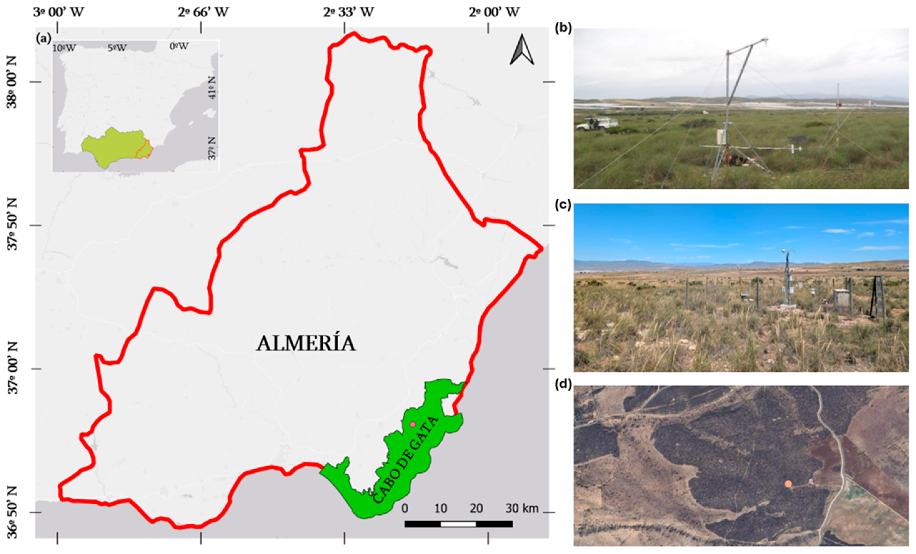
The study zone, designated as Balsa Blanca, is situated within the “Cabo de Gata-Níjar Natural Park” in the province of Almería (Andalucía), southeastern Spain (Figure 1). It is regarded as the only sub-desertic protected area in Europe, characterized by a semi-arid Mediterranean climate. Moreover, Balsa Blanca served as a calibration/validation site for the LST estimation algorithm of the ECOsystem Spaceborne Thermal Radiometer Experiment on Space Station (ECOSTRESS mission) from NASA [38].

Figure 1. (a) Overview of Balsa Blanca grassland eddy covariance flux site situated in “Cabo de Gata-Níjar Natural Park” (green zone); (b,c) representation of zone with in situ photo; (d) visualization of satellite image obtained from GoogleMaps; red point represents localization of eddy covariance tower site, named Blasa Blanca.

The study area is a tussock grassland steppe biome dominated by Stipa tenacissima L., which comprises 91% of the vegetation cover [21,32]. This species exhibits pronounced drought tolerance through several adaptive strategies, such as reducing light interception and photoinhibition [39], using non-rainfall water gains [40], and exhibiting a rapid photosynthetic response to rainfall events [41].

The climate in this region is classified as subtropical, dry, and semi-arid, with an average mean annual precipitation of 375 mm and an average annual temperature of approximately 18.1 °C. Rainfall exhibits significant interannual variability, as evidenced by records from the closest long-term meteorological station in Níjar (30 km), which reports an annual precipitation of 200 mm [42]. The fraction of vegetation cover is 60%, with an average canopy height of 0.7 m [21,32]. The soil in this region is classified as Mollic Leptosol and as sandy loam soil according to the USDA soil taxonomy, with a root zone depth ranging from 15 to 25 cm.

2.2. Field Measurements

The data were obtained during the growing season in 2011, spanning from 15 January (DOY 15) to 12 June (DOY 163). This period captures the majority of annual LE variability, despite representing only a subset of the growing season, which extends from fall to early summer [32]. The LE and H were measured by EC systems, which consisted of a three-dimensional sonic anemometer (CSAT-3, Campbell Scientific Ltd., Logan, UT, USA) to quantify wind speed and direction, and an LI-COR open-path infrared gas analyser (Li-7500, Campbell Scientific Ltd.) to determine water vapor and CO₂ concentrations. The GPP was derived as the difference between ecosystem respiration (Reco) and net ecosystem exchange (NEE). We used the nighttime partitioning method to partition NEE into GPP and Reco. The two EC system components were mounted at a height of 3.5 m and connected to a 10 Hz Campbell CR3000 datalogger (Campbell Scientific Ltd., USA). The datalogger calculated the means of EC measurements at 30 min intervals. The processing approaches of CO₂ and water vapor EC data followed the methodologies from related studies [43,44,45], which are consistent with the standard ICOS (Integrated Carbon Observation System) processing protocols. LE measurements were corrected for air density fluctuations caused by heat and water vapor transport [46] and for coordinate system rotation following the methods in Kowalski et al. [47] and McMillen [48]. To process high-frequency data, the Eddypro 5.0. software was used (Li-COR, Lincoln, NE, USA). Net radiation (Rn) was measured using the NR-Lite radiometer (Kipp & Zonen, Delft, The Netherlands).

Four soil heat flux (G) plates (HFP01SC; Campbell Scientific Inc., USA) were installed at a depth of 8 cm, with two positioned beneath the plant canopy and two beneath the bare soil surface. These plates were connected to a datalogger via a multiplexer. The surface G was calculated by combining the measured heat flux at 8 cm with the energy stored in the soil layer above the heat plate. This stored energy was estimated using soil temperature and soil moisture measurements. Soil temperature was measured using thermocouples (TCAV) installed at depths of 2 and 6 cm, and placed near the heat flux plates to ensure an accurate representation of the conditions above the measurement depth.

Continuous LST measurements were acquired by using Apogee IRTS-P broadband thermal infrared thermometers (Campbell Scientific Inc., USA), which operate within a full wavelength range of 6 to 14 µm. IRTs were installed to measure over bare soil, vegetation, and a composite of bare soil and vegetation. Incoming short-wave radiation was measured with an LP02 pyranometer (Campbell Scientific Inc., USA). All data were recorded and stored on a Campbell CR1000 data logger (Campbell Scientific Inc., USA).

Nevertheless, the use of EC resulted in an energy balance closure issue [49], whereby the turbulent flow, the sum of H and LE, was not equal to the available energy, defined as the difference between Rn and G. To rectify the energy balance closure errors, the Bowen ratio [50] was implemented for the LE and H variables at daily time steps. Furthermore, the residual methodology was employed to analyse the energy closure error, attributing it entirely to LE, calculated as the difference between all other variables ($Rn-G-H$). A statistical assessment was conducted using the raw data from the EC system, the data corrected using the Bowen ratio, and the data corrected using LE residues. The results were evaluated in comparison to the simulated data from SVEN, which were assessed using the RMSE and coefficient of determination (R²).

Air temperature (T_air) and relative humidity (RH) were measured with thermo hygrometers (HMP45C, Cambell Scientific Ltd., USA). Precipitation (P) was recorded using a tipping-bucket rain gauge with a resolution of 0.25 mm (ARG100 Campbell Scientific Inc., USA). Volumetric soil water content (SWC, m³·m⁻³) was measured using a time-domain reflectometry sensor (CS616, Cambell Scientific Ltd., USA) installed at a depth of 4 cm in both bare soil and vegetation-covered soil. All technical details regarding the sensors are based on the studies by Garcia et al. [32] and Morillas et al. [21].

2.3. Satellite Data

The Normalized Differentiation Vegetation Index (NDVI) data in 2011 were obtained from the Moderate Resolution Imaging Spectroradiometer (MODIS) Terra sensor product (MOD09Q1). This product is produced at a spatial resolution of 250 m and a temporal resolution of 8 days. The dataset includes the surface reflectance of the red and near-infrared bands, along with quality assessments for each band. Only NDVI values with optimal quality criteria [51], were used. To derive half-hourly NDVI estimates, linear interpolation and Savitzky–Golay smoothing [52] with a window size of 7 [53] were applied to 8-day NDVI data.

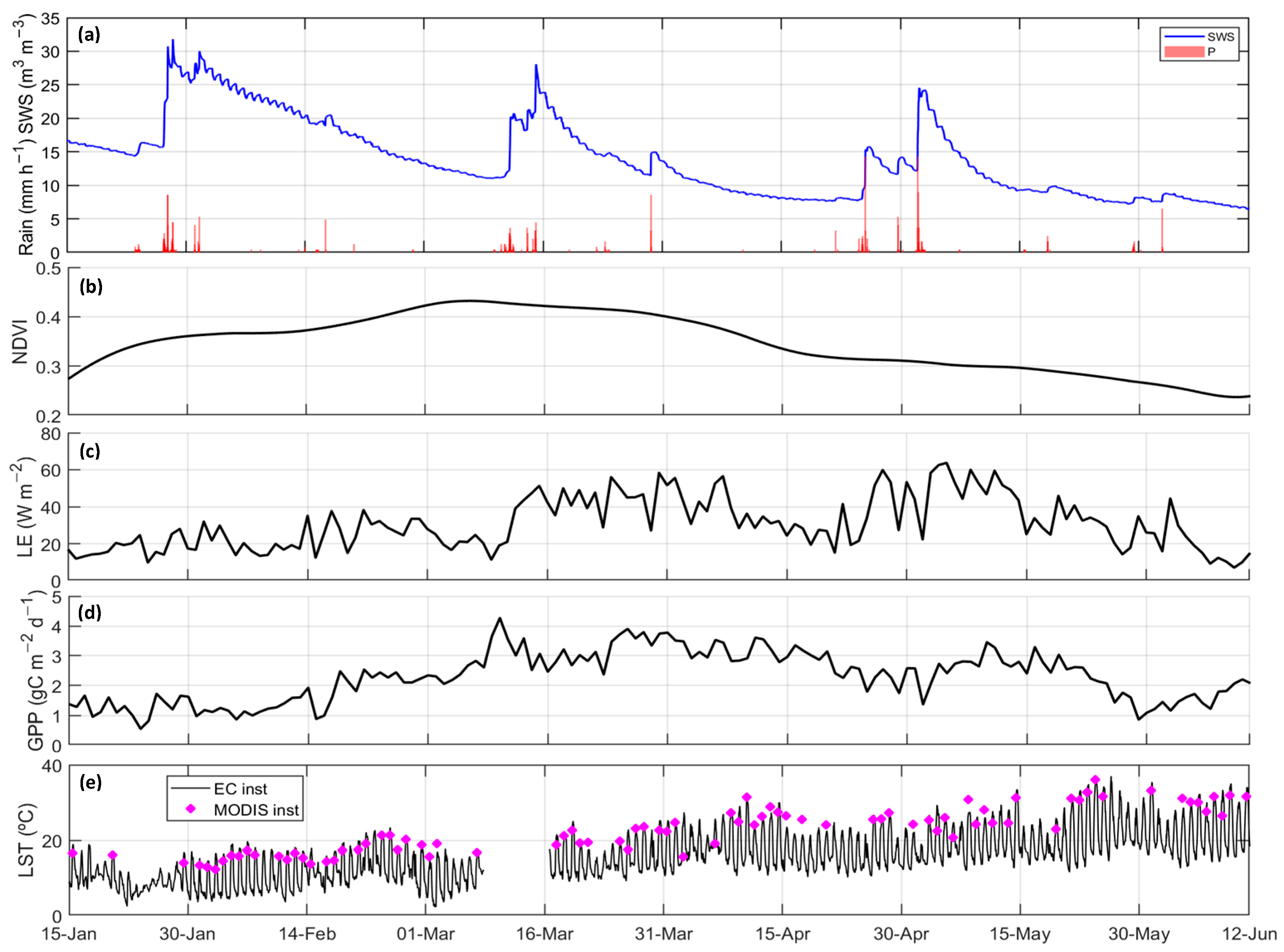
The daily LST data in 2011 were obtained from the MODIS Terra sensor product (MOD11A1), with a spatial resolution of 1 km. To calibrate the model, instantaneous LST was used as a reference. LST values that were classified as cloudy days were excluded [51] The time series of meteorological variables, energy, CO₂ fluxes, and NDVI at the field site are shown in Figure 2.

Figure 2. (a) Volumetric soil water content (SWC, m³·m⁻³) at a depth of 4 cm is represented by the blue line and precipitation is represented by the red bars (mm); (b) dynamics of Normalised Difference Vegetation Index (NDVI) during periods of analysis (half-daily data interpolated and smoothed); (c) latent heat flux (LE, evapotranspiration, W·m⁻²) at daily time step; (d) gross primary productivity (GPP, gC·m⁻²·d⁻¹); (e) black line represents instantaneous dynamic land surface temperature (LST, °C) observed from eddy covariance (EC) tower, while magenta points represent instantaneous LST (°C) observed from Moderate Resolution Imaging Spectroradiometer (MODIS) product. From 8 March to 16 March, there is a data gap due to technical issues of the EC tower.

3. Method

The SVEN model is a remote-sensing-based land surface model that simulates canopy radiation, energy, water, and carbon fluxes, as well as vegetation dynamics [22]. It builds on and expands the remote-sensing-based light use efficiency (LUE-GPP) model [27,54] and the Prestley–Taylor Jet Propulsion Laboratory (PT-JPL) ET model [29], rendering them dynamic. The model operates at half-hourly intervals and is capable of temporal interpolation, enabling the integration of the instantaneous land surface variables, including LST, R_n, SWC, LE, and GPP, into a continuous time series.

The model consists of three main modules: (a) Energy balance module estimates the LST and G using the land surface energy balance equations and the “force-restore” method [55,56]. It accounts for energy exchange between the ground and the soil–vegetation on the surface. (b) Water balance module incorporates the PT-JPL model to estimate LE and represents the upper soil column to simulate soil water dynamics and runoff generation. A simple “bucket” model is used to capture soil water constraints in this module; (c) CO₂ flux module uses the light use efficiency (LUE) model to estimate GPP and links it to LE through canopy biophysical constraints. All main equations used for each module are explained in the Supplementary Materials (Equations (S1)–(S5)).

3.1. Model Inputs

Meteorological data inputs for the SVEN model include short-wave incoming radiation (${SW}_{in}$), long-wave incoming radiation (${LW}_{in}$), air temperature ($T_{air}$), relative humidity (RH), wind speed (u), air pressure ($P_s$), and precipitation rate (P). In addition, NDVI derived from MODIS and canopy height ($h_c$) determined through literature review [21,32,57] are also needed to run the model. The initial parameters of the model include the canopy water storage (${CWS}_{in}$), soil water content (${SWC}_{in}$), surface temperature ($T_{s}o$), and deep soil temperature ($T_{d}o$), which were assumed following the supplement of Wang et al. [22] and assuming that the ${SWC}_{in}$ was at 25% of the maximum.

3.2. Model Parameters and Optimization

Table 1 displays the initial set of eight parameters for the soil texture and influences the dynamics of water storage, drainage in the “bucket” model, and the impact of the heat gradient in the “force-restore” method. The shape of the van Genuchen [58] soil–water retention relationship (n) was estimated using a look-up table [59]. The saturated volumetric soil moisture (${SWC}_s$, m³·m⁻³) and the residual volumetric soil moisture (${SWC}_r$, m³·m⁻³) were derived using a look-up table from [59]. The remaining soil and vegetation physical properties ($C_{sat}$, $C_{veg}$, b, ${SWC}_{max}$, and $K_s$) were derived through model calibration using instantaneous $LST$ data from daily MODIS observations and in situ LST measurements from EC. The incorporation of remotely sensed instantaneous data with in situ measurements enables the application of this method in regions with limited data availability.

Table 1. Summary of parameters in soil–vegetation–atmosphere energy, water, and CO₂ transfer model and their ranges for all soil and biome types. * Parameter values were determined by numerical optimisation. Other parameter values were obtained from literature. (-) Parameter is dimensionless with no units.

Parameter	Description	Value	Range	Unit	Reference
$C_{sat}$	The force-restore thermal coefficient for saturated soil	*	[4.00, 10.00]	10−6·K·m−2·J−1	[56]
b	The slope of the retention curve for the “force-restore” thermal coefficient	*	[4.61, 6.91]	(-)	[56]
n	The shape parameter of the van Genuchen ([58]) soil–water retention relationship	1.89	[1.01, 2.50]	(-)	[59]
${SWC}_s$	Saturated volumetric soil moisture	0.410	[0.360, 0.460]	m3·m−3	[59]
${SWC}_r$	Residual volumetric soil moisture	0.065	[0.034, 0.100]	m3·m−3	[59]
$K_s$	Saturated hydraulic conductivity	*	[1.00, 2.00]	mm·h−1	[59]
${LUE}_{max}$	Maximum light use efficiency	1.69	[0, 5.00]	gC·m−2·MJ−1	[60]
${SWC}_{max}$	Maximum soil water content	*	[1.00, 2.50]	10−3 m	[61]
$C_{veg}$	The “force-restore” thermal coefficient for vegetated surface	*	[1.00, 4.00]	10−6·K·m−2·J−1	[61]

The calibration of the $C_{sat}$, $C_{veg}$, b, ${SWC}_{max}$, and $K_s$ was conducted through Monte Carlo optimization, with reasonable ranges based on field measurements. A total of 5000 records were generated with a continuous uniform distribution following the specified ranges (Table 1). A statistical summary of the sampled parameter distributions is in Table S1, and a box-and-whisker plot to represent their variability is included in Figure S5. The optimization evaluation was conducted using the root mean square error (RMSE) between the observed and simulated values, with the minimum value utilized as the criterion for success. The ${LUE}_{max}$ was estimated through the optimization of the GPP module. Moreover, the ${LUE}_{max}$ was compared with the results in Zhou et al. [60], which indicated that fields exposed to incident solar radiation exhibited ${LUE}_{max}$ values approaching 1.69 gC·MJ⁻¹.

3.3. Model Simulation Assessment

The model was validated using independent EC data collected from the EC system, and the accuracy was evaluated at both half-hourly and daily time scales. The database was segmented into two sections: the first, comprising 70% of the data, was used for calibration and optimization parameters (from 15 January to 28 April), while the remaining 30% was allocated for validation (from 29 April to 12 June).

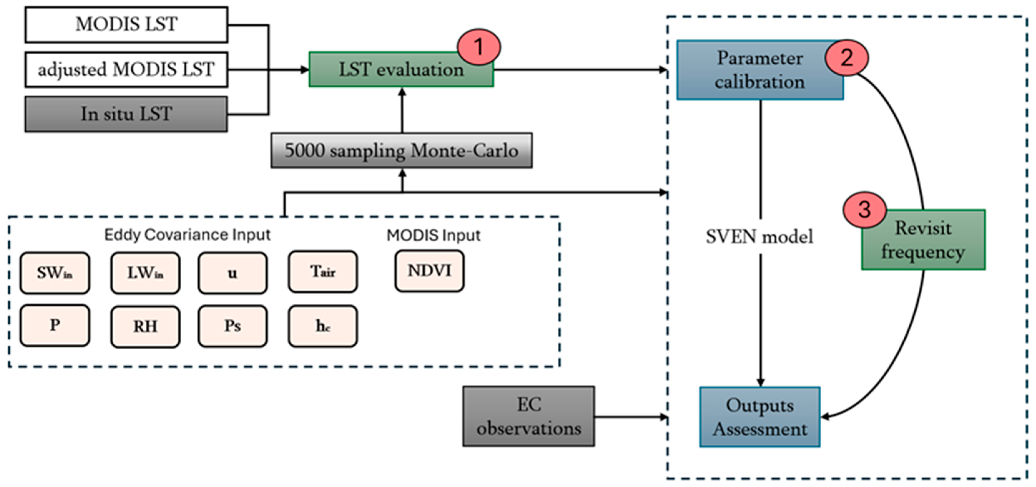
The optimization calibration was conducted on a daily time step with the use of instantaneous remote sensing data. Specifically, for each day, MODIS LST values (MOD11A1) were paired with in situ LST observations from the flux tower at the exact overpass time (date, hour, minute). The statistical evaluation was conducted by the RMSE, R² and Normalized Root Mean Square Error (NRMSE), Equations (1), (2) and (5), with SVEN simulations. Three distinct approaches were used to parameter calibration in Step 1 (Figure 3): (i) utilize LST data from in situ and selected samples that match the accurate pass time (date, hour, minute) of the MODIS sensors (in situ LST); (ii) use the MODIS LST product (MODIS LST); (iii) use adjusted MODIS LST, a simple linear regression was then fitted between MODIS and in situ LST. The regression coefficients were used to bias-correct the satellite product, generating an adjusted MODIS LST dataset aligned to ground-based observations. This adjusted dataset was then employed in the model calibration process (adjusted MODIS LST). After identifying the optimal LST data for parameter calibration, the model performance was subsequently evaluated, including RMSE, NRMSE, Bias, Mean Absolute Error (MAE), and R².

Figure 3. Workflow of calibration process for model parameters and assessment of model outputs. Step 1: Selection of optimal land surface temperature variable for parameter calibration. Step 2: Calibration of parameters through Bayesian uncertainty analysis. Step 3: Determination of optimal revisit pass frequency for satellite sensors. SW_in: Short Wave input radiation, LW_in: Long Wave input radiation, u: wind speed, T_air: air temperature, NDVI: Normalized Difference Vegetation Index, P: precipitation, RH: relative humidity, Ps: pressure, h_c: canopy height.

Based on the selected requisite parameters, we applied a Monte Carlo approach for model parameter optimization and uncertainty quantification (Step 2). The objective of using this approach and number of iterations is due to the computational limit. The uncertainty of the model was evaluated with the 95% confidence interval (CI). Specifically, we randomly sampled 5000 parameter sets according to the model parameter range (Table 1). We ran model simulations to assess the optimal parameter values as well as their 95% CI for model performance. In Table S1 (from Supplementary Materials) there is the statistic resume of the mean, standard deviation, minimum, maximum, and median values. In addition, Figure S5 shows the box-and-whisker plot. The process followed the next steps: (a) randomly sample parameters with the defined range; (b) run SVEN model with sampled values; (c) calculate RSME as performance metric from LST output.

While the temporal resolution for parameter calibration (Step 2) was set as daily, following the MODIS time scale. In Step 3, the parameter calibration during the satellite revisit period was performed by systematically varying the revisit intervals (1–16 days) and recalibrating the model for each case to identify the optimal revisit frequency and the point at which model accuracy begins to degrade. Parameter calibrations at different revisit frequencies were conducted by fitting the minus RMSE for LST observed data and LST simulated. Once best parameter fitted per each revisit frequencies, statistical evaluation was conducted by the RMSE, R², and NRMSE between the simulation outputs and in situ measurements, where timestep were half-hourly. The minimum sample size required for reliable calibration at a specific revisit frequency was determined.

Model performance was evaluated using root mean square error (RMSE), normalized RMSE (NRMSE), mean bias (Bias), mean absolute error (MAE), and the coefficient of determination (R²). Equations for these metrics are given below.

$$RMSE=\sqrt{{\displaystyle \frac{1}{n}}\sum _{i=1}^n\left(\widehat{y_i}-y_i\right)}$$

(1)

$$NRMSE={\displaystyle \frac{RMSE}{\underset{\_}{y}}}\times 100\%$$

(2)

$$Bias={\displaystyle \frac{1}{n}}\sum _{i=1}^n\left(\widehat{y_i}-y_i\right)$$

(3)

$$MAE={\displaystyle \frac{1}{n}}\sum _{i=1}^n\left|\widehat{y_i}-y_i\right|$$

(4)

$$R^2={\displaystyle \frac{{\sum }_{i=1}^n\left(y_i-\underset{\_}{y}\right)\left(\widehat{y_i}-\underset{\_}{\widehat{y}}\right)}{\sqrt{{\sum }_{i=1}^n{\left(y_i-\underset{\_}{y}\right)}^2}\sqrt{{\sum }_{i=1}^n{\left(\widehat{y_i}-\underset{\_}{\widehat{y}}\right)}^2}}}$$

(5)

where $y_i$ is the observed value at sample i (e.g., in situ measurement from flux tower); $\widehat{y_i}$ is the simulated or estimated value at sample i (e.g., model output or MODIS-derived value); $\underset{\_}{y}$ is the mean of observed values; $\underset{\_}{\widehat{y}}$ is the mean of simulated/estimated values; and $n$ is the total number of paired samples.

4. Results

4.1. Accuracy of MODIS LST Data and Flux Simulations

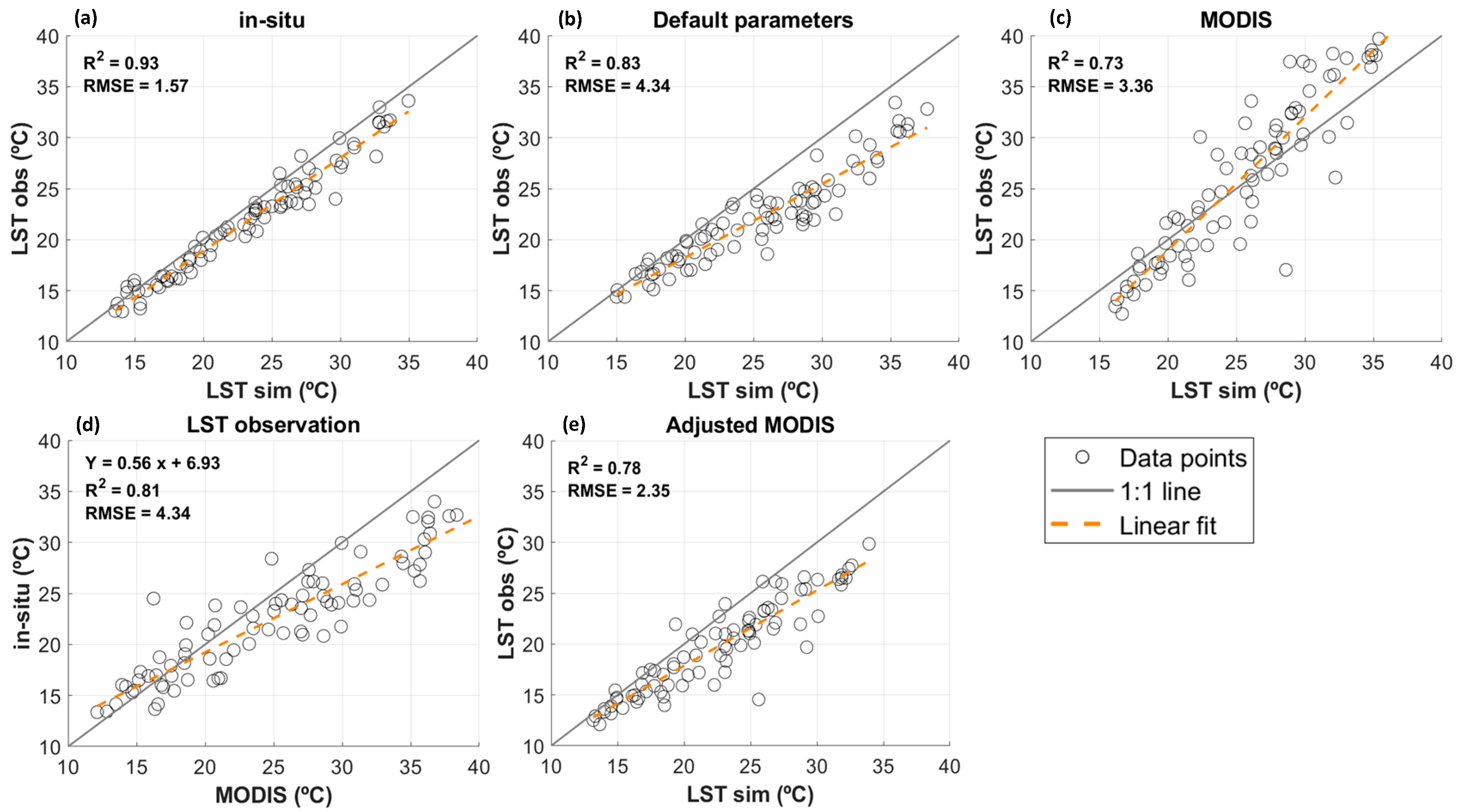
Using the default parameter set resulted in large errors, with an RMSE of 4.34 °C (Figure 4b). Similarly, calibration with the raw MODIS LST product showed substantial bias (RMSE = 3.36 °C; Figure 4c). However, MODIS and in situ LST were strongly correlated (Figure 4d), enabling a regression-based bias correction. Applying this adjustment substantially improved consistency with simulated LST, reducing the RMSE to 2.35 °C (Figure 4e), and yielding performance much closer to that obtained with in situ calibration.

Figure 4. Scatterplot of simulated instantaneous LST from SVEN compared to observed LST at calibration. (a) Observed LST data obtained from in situ measurement; (b) observed data obtained from in situ LST sensor compared with simulated LST using default parameters without being calibrated; (c) observed LST data obtained from MODIS; (d) relationship between in situ and MODIS LST observation; (e) observed data obtained from adjusted MODIS product using linear regression. Grey line denotes 1:1 reference and orange dashed line denotes least-squares linear regression (best-fit).

The comparison of calibrated parameters with in situ LST and adjusted MODIS LST is presented in Table 2. The adjusted MODIS LST-based flux simulations demonstrated similar accuracies in LST and SWC compared to simulations based on in situ LST measurements. To further understand the relationship between the LST and calibrated parameters in the model, we simulated C_veg values and errors of LST through the Bayesian analysis (Step 2 in Figure 3). The C_veg exhibited the highest sensitivity to LST RMSE, with errors increasing when C_veg values exceed 3.5·10⁻⁶·K·m⁻²·J⁻¹ (Figure S1a). This can explain the non-compilation of the MODIS scenario, which is linked to the high value of C_veg. In addition, the uncertainty of the model was accounted for through LST time series with a 95% confidence interval (Figure S1b). The model tends to overestimate at LST peaks and underestimate at LST troughs, highlighting its sensitivity to LST parameters.

Table 2. Summary of calibrated parameters through in situ land surface temperature (LST), and adjusted Moderate Resolution Imaging Spectroradiometer LST (adjusted MODIS), and evaluation results of different LST source-based calibrated models. (-) Parameter is dimensionless with no units. C_sat—force-restore thermal coefficient for saturated soil, SWC_max—maximum soil water content, C_veg—force-restore thermal coefficient for vegetated surface, K_s—saturated hydraulic conductivity, LE—latent heat flux, Rn—net radiation, H—sensible heat flux, SWC—soil water content.

		In Situ		Adjusted MODIS
Parameters	Csat (10−6·K·m−2·J−1)	9.711		9.595
	b (-)	5.817		5.632
	SWCmax (m3·m−3)	1.082		2.292
	Cveg (10−6·K·m−2·J−1)	2.306		2.190
	Ks (mm·h−1)	1.949		1.016
		RMSE	NRMSE (%)	RMSE	NRMSE (%)
Validation	LST (°C)	2.15	8.43	1.99	7.84
	LE (W·m−2)	26.15	10.49	28.21	11.32
	Rn (W·m−2)	53.12	5.72	52.71	5.67
	H (W·m−2)	49.05	7.52	50.90	7.81
	SWC (m3·m−3)	1.99	11.03	1.19	6.59

4.2. Validation at the Half-Hourly and Daily Time Scale

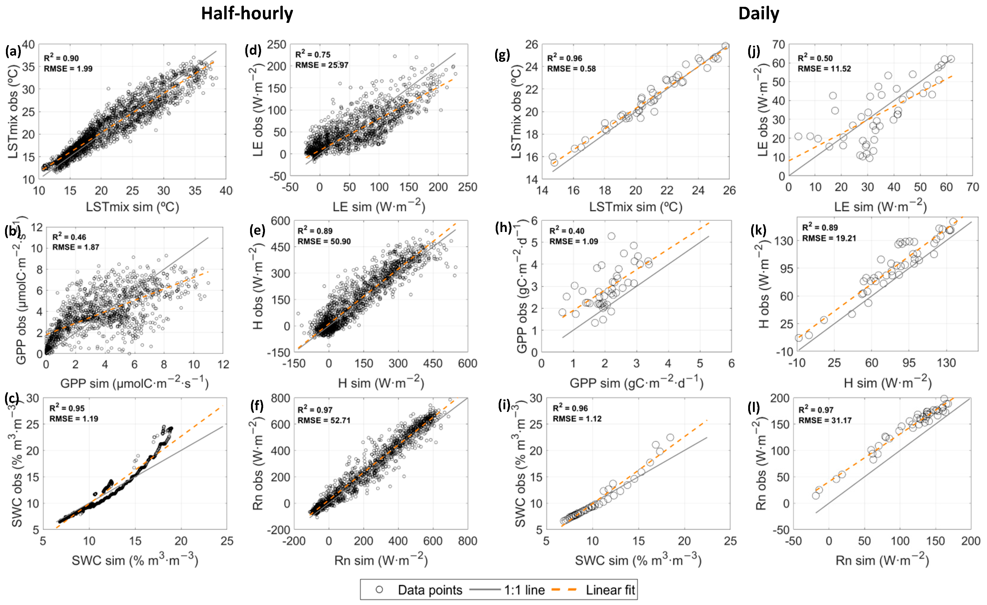
Based on the assessment results (Table 2), we evaluated the model at half-hourly and daily time scales using the parameters obtained from MODIS-adjusted LST (Table 3). The observed LST data at three distinct scenarios, including bare soil, vegetated soil, and a combination of vegetated and bare soil, were used as the reference. Only the mixed scenario was considered for comparison, as it showed the highest similarity to the MODIS LST product with 1 km spatial resolution. Furthermore, LST simulations from the SVEN model were highly consistent with observed LST in overall performance and time series (Figure 5a and Figure S2a).

Table 3. Performance of Soil-Vegetation-atmosphere Energy, water, and CO₂ traNsfer (SVEN) model in estimating land surface temperature (LST) of mixed canopy (LST mix), bare soil (LST soil) and vegetation canopy (LST canopy), latent heat flux (LE), net radiation (Rn), sensible heat flux (H), gross primary production (GPP), and soil water content (SWC) at half-hourly and daily time scales compared to eddy covariance measurements. Results were evaluated between 29 April and 12 June. A total of 2160 samples were used for validation at a half-hourly scale, and 45 samples were used for validation at a daily scale. Unit of half-hourly GPP is µmolC·s^−1·m⁻², and unit of daily GPP is gC·d⁻¹m⁻².

Timescale	Statistics	LST Mix (°C)	LST Soil (°C)	LST Canopy (°C)	LE (W·m−2)	Rn (W·m−2)	H (W·m−2)	GPP (µmolC·s−1·m−2 or gC·d−1·m−2)	SWC (m3·m−3)
Half-hourly	RMSE	1.99	2.63	2.10	25.97	52.71	50.9	1.87	1.19
	MAE (%)	1.59	2.09	1.65	16.54	39.56	34.42	1.46	0.77
	bias	0.23	1.12	0.01	−1.37	29.81	15.19	−0.18	−0.05
	R2	0.90	0.89	0.90	0.75	0.97	0.89	0.46	0.95
	NRMSE (%)	7.84	8.94	8.54	10.81	5.67	7.81	24.03	6.59
Daily	RMSE	0.58	1.29	0.56	11.52	31.17	19.21	1.09	1.12
	MAE (%)	0.47	1.19	0.45	9.42	29.81	15.89	0.87	0.76
	bias	0.23	1.12	−0.01	−1.38	29.81	15.2	−0.82	−0.04
	R2	0.96	0.94	0.96	0.50	0.97	0.89	0.40	0.96
	NRMSE (%)	5.68	12.22	5.45	21.88	16.93	13.10	37.33	6.53

Figure 5. Relationship between simulated (sim) and observed data during the validation period (29 April–12 June) at half-hourly and daily time scales. Left panels (a–f) show half-hourly results, and right panels (e–l) show daily results. (a,g) Land surface temperature (LST, °C), (b,h) gross primary productivity (GPP, µ·molsC·s⁻¹·m⁻², g·C·d⁻¹·m⁻²), (c,i) soil moisture (SWC, m³·m⁻³), (d,j) evapotranspiration or latent heat flux (LE, W·m⁻²), (e,k) sensible heat flux (H, W·m⁻²), (f,l) net radiation (R_n, W·m⁻²). Grey line denotes 1:1 reference and orange dashed line denotes least-squares linear regression (best-fit).

Upon examination of Rn at the daily time scale (Figure 5l), a slight offset was discernible between the simulated and observed values, despite the maintenance of a robust linear correlation (0.97). LE was found to be underestimated when SW_in values were close to zero. However, at 40 W·m⁻², the performance of the model was variable, indicating a potential point at which the forecast should be adjusted. On the daily time scale, the RMSE was reduced to approximately half compared to the half-hourly scale, while NRMSE increased for all parameters except SWC. The time series panels related to energy balance (Figures S2b–d) exhibited negative values during the night.

The SWC simulations demonstrated satisfactory accuracy with R² > 0.9 and RMSE < 1.2% in both half-hourly and daily time scales (Figure 5c,i). The precipitation effect on SWC was effectively simulated, while the impacts of the first two precipitation events on SWC were not simulated accurately due to the poor performance of the SWC simulations during the initial peak period (Figure S2f). Although the model exhibited an underestimation of the SWC in the initial short period (before 17 May), it captured precipitation, evapotranspiration, and soil infiltration processes.

The GPP simulations showed a poor correlation to observations from EC, with R² = 0.46 for half-hourly time scale and R² = 0.40 for daily time scale (Figure 5b,h). Nevertheless, the RMSE of 1.87 µmolsC·s⁻¹·m⁻² at half-hourly time scale and 1.09 gC·d⁻¹·m⁻² at daily time scale were acceptable due to the pronounced fluctuations in carbon assimilation rates under different lighting conditions and stages of the phenological cycle. At the half-hourly scale, the model tends to underestimate the GPP at the low GPP value (<3.00 µmolsC·s⁻¹·m⁻²), while for higher values the prediction changes to an overestimation (Figure 5b).

The model simulations exhibited approximately 20–22% of errors when validated against the EC observation. This might originate from error propagation during parameter calibration, introducing uncertainty into the simulated time series. After comprehensive NRMSE evaluation, all energy balance variables (LE, H, Rn) attained values remained within the range of uncertainties reported for the EC. However, the GPP simulations showed a marginal NRMSE exceedance of 2.03–15.33% above the EC uncertainty level of 22%.

4.3. Revisit Satellite Frequency for Parameter Calibration

We further investigated and determined the optimal operational revisit time for satellite products. The time windows for parameter calibration ranged from 2 to 16 days. The calibration and validation results of all parameters at different satellite pass frequencies are shown in Table 4.

Table 4. Summary of calibrated parameters and model validation results based on different satellite revisit pass frequencies with sample size (n) of each calibration scheme during period from 15 January to 28 April. (-) Parameter is dimensionless with no units. Calibration period is 15 January to 28 April, and validation period is 29 April to 12 June. (RMSE—∆ vs. 1-day) reflects absolute and relative error compared to 1-day values.

Revisit Frequency	n	Optimized Parameter Values					Simulation Performance (RMSE—∆ vs. 1-Day)
		Csat (10−6·K·m−2·J−1)	b (-)	SWCmax (m3·m−3)	Cveg (10−6·K·m−2·J−1)	Ks (mm·h−1)	LST (°C)	LE (W·m−2)	Rn (W·m−2)	H (W·m−2)	SWC (m3·m−3)
1 day	56	9.595	5.632	2.292	2.194	1.016	1.99	28.21	52.71	50.89	1.19
2 days	28	9.004	5.586	2.308	2.383	1.016	2.10 (+0.11 +5.50%)	28.16 (−0.05 −0.18%)	52.97 (+0.26 +0.49%)	50.22 (−0.67 −1.32%)	1.20 (+0.01 +0.84%)
4 days	14	9.571	6.401	2.439	2.397	1.083	2.18 (+0.19 +9.50%)	28.01 (−0.2 −0.71%)	52.88 (+0.17 +0.32%)	50.16 (−0.73 −1.43%)	1.29 (+0.1 +8.40%)
6 days	9	8.978	6.797	2.352	2.505	1.001	2.25 (+0.26 +13.10%)	28.26 (+0.05 +0.18%)	52.93 (+0.22 +0.42%)	51.32 (+0.43 +0.84%)	1.25 (+0.06 +5.04%)
8 days	7	9.514	6.604	2.490	2.403	1.173	2.20 (+0.21 +10.60%)	27.77 (−0.44 −1.56%)	52.93 (+0.22 +0.42%)	50.15 (−0.74 −1.45%)	1.32 (+0.13 +10.92%)
16 days	4	9.801	4.849	2.361	3.906	1.880	3.15 (+1.16 +58.30%)	27.67 (−0.54 −1.91%)	60.10 (+7.39 +14.02%)	81.33 (+30.44 +59.82%)	1.44 (+0.25 +21.01%)

The parameter sensitivity to observation frequency varies in Table 4. Specifically, some parameters ($C_{sat}$ and SWC_max) maintained relatively stable values even with reduced observations. In contrast, other parameters ($K_s$, $C_{veg}$, and b) exhibited notable divergence when calibration samples were limited to four. The model accuracy, as quantified by both RMSE and NRMSE, decreased with fewer calibration observations that resulted from the coarser temporal resolution.

LST and H were the most frequently dependent variables affecting model outcomes (Table 4). The LST RMSE exhibited a progressive increase with sample size reduction, reaching an error range of 2.0 to 2.3 °C at seven samples and increasing to 3.0 °C when sample size decreased to four. Similarly, the simulation error of H nearly doubled when parameters were calibrated with only four samples. In contrast, the R_n and SWC showed lower sensitivity to sample size reduction, with an increasing error of 7.49 W·m⁻² and 0.25 m³·m⁻³, respectively. Notably, LE maintained exceptional stability across all calibration scenarios, showing its independence of sample size.

The simulations ran with the parameters calibrated with four samples, exhibited irregularities in the compilation on 30 May and 7 June due to the presence of outliers. The application of the z-score outlier function with a threshold of three to the LST, LE, H, Rn, and SWC variables identified 0.79%, 0.56%, 0.88%, 0.19%, and 2.08%, respectively, as outliers. Once outliers were removed, the remaining data were subjected to statistical analysis. Even after the removal of outliers, the scenario with only four samples at parameter calibration exhibited suboptimal statistical performance.

The problem seems to be concentrated in the parameters b, $K_s$, and $C_{veg}$ since they presented the largest discrepancy with respect to the other scenarios (Table 4). In addition, the LST and H variables showed the lowest precision. Inaccurate estimation of the parameters b, $K_s$, and $C_{veg}$ will be reflected in the “force-restore” method, responsible for the LST and H estimation.

5. Discussion

This study explored the potential of calibrating the SVEN model using MODIS LST to estimate land surface fluxes in dryland environments. Our findings demonstrate the effectiveness of incorporating satellite-derived LST for improving SVEN model performance and identifying optimal satellite revisit frequencies for reliable half-hourly flux estimations. The discussion below presents a detailed comparison with existing models, examines model strengths and weaknesses, highlights avenues for improvement, and considers scalability challenges.

5.1. Comparison with Existing Surface Flux Models

The SVEN model demonstrated strong performance in estimating surface fluxes (LE, H, Rn) at both half-hourly and daily timescales in dryland conditions. Compared to earlier applications (e.g., [22]) in energy-limited ecosystems, our study confirmed the value of satellite LST integration for enhancing model accuracy in water-limited environments.

Benchmarking against Morillas et al. [21], who applied a two-source model in the same study site, our SVEN model yielded significantly lower RMSE and higher correlation coefficients—approximately double—indicating improved reliability under challenging dryland conditions. Our NRMSE for LE remained below 22%, whereas Morillas et al. reported ~90% relative error at the daily scale.

Thermal-based models like those by Kustas and Norman [62] depend heavily on instrument accuracy. In contrast, vegetation-driven models such as PT-JPL [29] are less sensitive to radiometric temperature quality. While PT-JPL achieved reliable H estimations via canopy–soil disaggregation [21], our SVEN model’s H performance was similarly robust, affirming effective flux component separation.

5.2. Further Improvements for Surface Flux Simulations

The eddy covariance station is located in a semi-arid site characterized by low latent heat fluxes. We tested common energy-balance closure corrections (Bowen-ratio and residual methods) on the full dataset (15 January–12 June; Figure S4). The Bowen-ratio correction resulted in poorer agreement (higher RMSE, lower R²), whereas the uncorrected EC fluxes showed the best correspondence with the SVEN simulations calibrated using LST. The eddy covariance closure residual at the site is ≈22%, consistent with previous reports [21,24,32]. Notably, model NRMSE for LST, LE, H and Rn are all <10%—smaller than the eddy covariance system’s typical systematic uncertainty—indicating that model–data discrepancies are comparable to measurement uncertainty.

Although SVEN performed well for energy fluxes, the CO₂ flux module showed suboptimal accuracy in drylands. This may be due to oversimplified LUE parameterization and structure. Future enhancements could be drawn from models like the two-leaf LUE (TL-LUE) model [60], which disaggregates GPP by sunlit and shaded leaves, improving robustness against PAR variation.

Significant uncertainty stemmed from NDVI-based vegetation indices (VI). Substituting with LAI and incorporating soil resistivity corrections—as proposed by Kustas et al. [57]—could reduce RMSE by over 40%. Incorporating hyperspectral or high-resolution UAV data can also improve vegetation characterization for GPP and ET simulations [63,64]. Additionally, treating the canopy and substrate coefficients (C_veg, C_sat) as temperature-dependent parameters rather than constants would reduce LST decoupling artifacts, especially near critical thresholds like 20 °C.

5.3. Remotely Sensed Surface Temperature for Model Optimization

LST serves as a crucial integrative variable reflecting land–atmosphere interactions [65], affecting H and LE partitioning [62], and plays an important role in drought monitoring, urban heat assessment, and climate modelling (e.g., [66,67]). Our LST estimation achieved normalized daily errors below 6%, outperforming previous studies (e.g., [32,68]). However, MODIS-derived LST lacks sufficient soil water content (SWC) sensitivity. Integrating multiple remote sensing products (e.g., LST and SWC), as in Wang et al. [22], using multi-objective optimization could improve SWC estimation and enhance LE simulations.

We further recommend adopting high-resolution remote sensing (e.g., ECOSTRESS) for parameter calibration. For example, ECOSTRESS LST data show RMSE of ~2 °C and strong agreement with eddy covariance observations [69], in addition, Fisher et al. demonstrated the high agreement (R² = 0.89, NRMSE = 8%) between the ECOSTRESS product and 82 global EC stations [69]. Moreover, ensuring a revisit interval below five days—as shown by Alfieri et al. [33]—is critical for maintaining LE simulation errors below 20%.

Our study confirmed that an eight-day calibration window enables reliable half-hourly LE simulations for ~100 days, with NRMSE up to 10.5%. Reduced revisit frequency correlates with increased error, underscoring the importance of frequent satellite observations for parameter stability.

5.4. Scalability Challenges

This study focuses on the Balsa Blanca site, a representative locality within the Natural Park of Cabo de Gata. SVEN provides a favourable balance between input parsimony and predictive accuracy, offering computationally efficient simulations. However, applying the model at larger scales requires careful evaluation because calibrated parameters are site-specific and the study area is an extreme, sub-desert environment.

Two critical issues must be addressed for regional application. First, parameter calibration must accommodate variability in plant functional types and soil properties (e.g., stratified or multi-PFT parameter sets), since biophysical parameters will differ across vegetation and soil classes. Second, gridded meteorological forcings (e.g., ERA5) should be bias-corrected against local observations to avoid propagating systematic forcing errors into model outputs (radiation, precipitation, temperature, humidity, wind). Addressing these points will reduce structural and forcing-related uncertainties when upscaling.

Overall, SVEN’s simplicity is an advantage for data-limited regions, but its scalability depends on (i) representing sub-grid heterogeneity and (ii) developing robust, transferable calibration strategies. Future studies should establish transferable parameterization schemes while preserving the biophysical processes in model.

6. Conclusions

Satellite remote sensing plays a vital role in providing data for regions lacking in situ observations. However, its utility is limited to clear-sky conditions and overpass times. In this context, process-based models serve as effective tools to complement satellite observations by high-resolution filling spatial and temporal data gaps. This study focused on a dynamic soil–vegetation–atmosphere transfer model, which simulates energy and water balances, and CO₂ fluxes. The model was parameterized using both in situ and MODIS remotely sensed LST data for comparison. The MODIS LST data show high correction but large bias with in situ LST. With linear-corrected MODIS LST data, the accuracy obtained in terms of RMSE for LST, LE, Rn, H, GPP, and SWC were 1.99 °C, 25.97 W·m⁻², 52.71 W·m⁻², 50.90 W·m⁻², 1.87 µmolsC·s⁻¹·m⁻², and 1.19 m³·m⁻³, on a half-hourly time scale, respectively. Increasing the number of days between satellite revisits causes a reduction in the number of calibration samples, which reduces the accuracy of the model. In addition, we observed that for a fixed revisit frequency, the calibration period should be at least eight days to ensure sufficient sample sizes and did not significantly affect the accuracy of the model, increasing the RMSE of the variables by only 0.42 to 10.53% at the half-hourly time scale. Overall, the integration of remotely sensed LST data for model calibration—validated against in situ eddy covariance data—demonstrated that the dynamic model provides accurate and reliable simulations of energy balance, water fluxes, and carbon exchange. These findings highlight the model’s potential as a robust tool for near-instantaneous surface flux estimation in data-scarce, semi-arid ecosystems such as Europe’s only sub-desertic protected area.

References

- Swift, J.; DM, E.M.C. Climate Variability, Ecosystem Stability and the Implications for Range and Livestock Development. Range Ecol. Disequilibrium Overseas Dev. Inst. Lond. 1993, 31–41. [Google Scholar]
- Glenn, E.P.; Huete, A.R.; Nagler, P.L.; Hirschboeck, K.K.; Brown, P. Integrating Remote Sensing and Ground Methods to Estimate Evapotranspiration. Crit. Rev. Plant Sci. 2007, 26, 139–168. [Google Scholar] [CrossRef]
- Giorgi, F.; Lionello, P. Climate Change Projections for the Mediterranean Region. Glob. Planet. Change 2008, 63, 90–104. [Google Scholar] [CrossRef]
- Baldocchi, D. “Breathing” of the Terrestrial Biosphere: Lessons Learned from a Global Network of Carbon Dioxide Flux Measurement Systems. Aust. J. Bot. 2008, 56, 1–26. [Google Scholar] [CrossRef]
- Brogaard, S.; Runnstrom, M.; Seaquist, J. Primary Production of Inner Mongolia, China, between 1982 and 1999 Estimated by a Satellite Data-Driven Light Use Efficiency Model. Glob. Planet. Change 2005, 45, 313–332. [Google Scholar] [CrossRef]
- Beer, C.; Reichstein, M.; Tomelleri, E.; Ciais, P.; Jung, M.; Carvalhais, N.; Rödenbeck, C.; Arain, M.A.; Baldocchi, D.; Bonan, G.B.; et al. Terrestrial Gross Carbon Dioxide Uptake: Global Distribution and Covariation with Climate. Science 2010, 329, 834–838. [Google Scholar] [CrossRef]
- Ito, A.; Inatomi, M. Water-Use Efficiency of the Terrestrial Biosphere: A Model Analysis Focusing on Interactions between the Global Carbon and Water Cycles. J. Hydrometeorol. 2012, 13, 681–694. [Google Scholar] [CrossRef]
- Jung, M.; Reichstein, M.; Margolis, H.A.; Cescatti, A.; Richardson, A.D.; Arain, M.A.; Arneth, A.; Bernhofer, C.; Bonal, D.; Chen, J.; et al. Global Patterns of Land-Atmosphere Fluxes of Carbon Dioxide, Latent Heat, and Sensible Heat Derived from Eddy Covariance, Satellite, and Meteorological Observations. J. Geophys. Res. 2011, 116, G00J07. [Google Scholar] [CrossRef]
- Fisher, J.B.; Melton, F.; Middleton, E.; Hain, C.; Anderson, M.; Allen, R.; McCabe, M.F.; Hook, S.; Baldocchi, D.; Townsend, P.A.; et al. The Future of Evapotranspiration: Global Requirements for Ecosystem Functioning, Carbon and Climate Feedbacks, Agricultural Management, and Water Resources. Water Resour. Res. 2017, 53, 2618–2626. [Google Scholar] [CrossRef]
- Denis, G.; Claverie, A.; Pasco, X.; Darnis, J.-P.; De Maupeou, B.; Lafaye, M.; Morel, E. Towards Disruptions in Earth Observation? New Earth Observation Systems and Markets Evolution: Possible Scenarios and Impacts. Acta Astronaut. 2017, 137, 415–433. [Google Scholar] [CrossRef]
- Anderson, M.; Norman, J.; Kustas, W.; Houborg, R.; Starks, P.; Agam, N. A Thermal-Based Remote Sensing Technique for Routine Mapping of Land-Surface Carbon, Water and Energy Fluxes from Field to Regional Scales. Remote Sens. Environ. 2008, 112, 4227–4241. [Google Scholar] [CrossRef]
- Bhattacharya, B.K.; Mallick, K.; Desai, D.; Bhat, G.S.; Morrison, R.; Clevery, J.R.; Woodgate, W.; Beringer, J.; Cawse-Nicholson, K.; Ma, S.; et al. A Coupled Ground Heat Flux–Surface Energy Balance Model of Evaporation Using Thermal Remote Sensing Observations. Biogeosciences 2022, 19, 5521–5551. [Google Scholar] [CrossRef]
- Mallick, K.; Baldocchi, D.; Jarvis, A.; Hu, T.; Trebs, I.; Sulis, M.; Bhattarai, N.; Bossung, C.; Eid, Y.; Cleverly, J.; et al. Insights Into the Aerodynamic Versus Radiometric Surface Temperature Debate in Thermal-Based Evaporation Modeling. Geophys. Res. Lett. 2022, 49, e2021GL097568. [Google Scholar] [CrossRef]
- Bai, Y.; Bhattarai, N.; Mallick, K.; Zhang, S.; Hu, T.; Zhang, J. Thermally Derived Evapotranspiration from the Surface Temperature Initiated Closure (STIC) Model Improves Cropland GPP Estimates under Dry Conditions. Remote Sens. Environ. 2022, 271, 112901. [Google Scholar] [CrossRef]
- Bayat, B.; Van Der Tol, C.; Verhoef, W. Integrating Satellite Optical and Thermal Infrared Observations for Improving Daily Ecosystem Functioning Estimations during a Drought Episode. Remote Sens. Environ. 2018, 209, 375–394. [Google Scholar] [CrossRef]
- Kustas, W.; Anderson, M. Advances in Thermal Infrared Remote Sensing for Land Surface Modeling. Agric. For. Meteorol. 2009, 149, 2071–2081. [Google Scholar] [CrossRef]
- Ryu, Y.; Baldocchi, D.D.; Kobayashi, H.; Van Ingen, C.; Li, J.; Black, T.A.; Beringer, J.; Van Gorsel, E.; Knohl, A.; Law, B.E.; et al. Integration of MODIS Land and Atmosphere Products with a Coupled-Process Model to Estimate Gross Primary Productivity and Evapotranspiration from 1 Km to Global Scales: GLOBAL GPP AND ET. Glob. Biogeochem. Cycles 2011, 25, 271–284. [Google Scholar] [CrossRef]
- Amthor, J.S.; Chen, J.M.; Clein, J.S.; Frolking, S.E.; Goulden, M.L.; Grant, R.F.; Kimball, J.S.; King, A.W.; McGuire, A.D.; Nikolov, N.T.; et al. Boreal Forest CO2 Exchange and Evapotranspiration Predicted by Nine Ecosystem Process Models: Intermodel Comparisons and Relationships to Field Measurements. J. Geophys. Res. 2001, 106, 33623–33648. [Google Scholar] [CrossRef]
- Reichstein, M.; Falge, E.; Baldocchi, D.; Papale, D.; Aubinet, M.; Berbigier, P.; Bernhofer, C.; Buchmann, N.; Gilmanov, T.; Granier, A.; et al. On the Separation of Net Ecosystem Exchange into Assimilation and Ecosystem Respiration: Review and Improved Algorithm. Glob. Change Biol. 2005, 11, 1424–1439. [Google Scholar] [CrossRef]
- Sitch, S.; Smith, B.; Prentice, I.C.; Arneth, A.; Bondeau, A.; Cramer, W.; Kaplan, J.O.; Levis, S.; Lucht, W.; Sykes, M.T.; et al. Evaluation of Ecosystem Dynamics, Plant Geography and Terrestrial Carbon Cycling in the LPJ Dynamic Global Vegetation Model. Glob. Change Biol. 2003, 9, 161–185. [Google Scholar] [CrossRef]
- Morillas, L.; Leuning, R.; Villagarcía, L.; García, M.; Serrano-Ortiz, P.; Domingo, F. Improving Evapotranspiration Estimates in Mediterranean Drylands: The Role of Soil Evaporation: Evapotranspiration Estimation in Mediterranean Dry Lands. Water Resour. Res. 2013, 49, 6572–6586. [Google Scholar] [CrossRef]
- Wang, S.; Garcia, M.; Ibrom, A.; Bauer-Gottwein, P. Temporal Interpolation of Land Surface Fluxes Derived from Remote Sensing—Results with an Unmanned Aerial System. Hydrol. Earth Syst. Sci. 2020, 24, 3643–3661. [Google Scholar] [CrossRef]
- Baldocchi, D.D. Assessing the Eddy Covariance Technique for Evaluating Carbon Dioxide Exchange Rates of Ecosystems: Past, Present and Future. Glob. Change Biol. 2003, 9, 479–492. [Google Scholar] [CrossRef]
- Wang, S.; Garcia, M.; Bauer-Gottwein, P.; Jakobsen, J.; Zarco-Tejada, P.J.; Bandini, F.; Paz, V.S.; Ibrom, A. High Spatial Resolution Monitoring Land Surface Energy, Water and CO2 Fluxes from an Unmanned Aerial System. Remote Sens. Environ. 2019, 229, 14–31. [Google Scholar] [CrossRef]
- Kalma, J.D.; McVicar, T.R.; McCabe, M.F. Estimating Land Surface Evaporation: A Review of Methods Using Remotely Sensed Surface Temperature Data. Surv. Geophys. 2008, 29, 421–469. [Google Scholar] [CrossRef]
- Wang, K.; Dickinson, R.E. A Review of Global Terrestrial Evapotranspiration: Observation, Modeling, Climatology, and Climatic Variability. Rev. Geophys. 2012, 50, 2011RG000373. [Google Scholar] [CrossRef]
- Carlson, T.N.; Gillies, R.R.; Schmugge, T.J. An Interpretation of Methodologies for Indirect Measurement of Soil Water Content. Agric. For. Meteorol. 1995, 77, 191–205. [Google Scholar] [CrossRef]
- Sandholt, I.; Rasmussen, K.; Andersen, J. A Simple Interpretation of the Surface Temperature/Vegetation Index Space for Assessment of Surface Moisture Status. Remote Sens. Environ. 2002, 79, 213–224. [Google Scholar] [CrossRef]
- Fisher, J.B.; Tu, K.P.; Baldocchi, D.D. Global Estimates of the Land–Atmosphere Water Flux Based on Monthly AVHRR and ISLSCP-II Data, Validated at 16 FLUXNET Sites. Remote Sens. Environ. 2008, 112, 901–919. [Google Scholar] [CrossRef]
- Mu, Q.; Zhao, M.; Running, S.W. Improvements to a MODIS Global Terrestrial Evapotranspiration Algorithm. Remote Sens. Environ. 2011, 115, 1781–1800. [Google Scholar] [CrossRef]
- Running, S.W.; Nemani, R.R.; Heinsch, F.A.; Zhao, M.; Reeves, M.; Hashimoto, H. A Continuous Satellite-Derived Measure of Global Terrestrial Primary Production. BioScience 2004, 54, 547. [Google Scholar] [CrossRef]
- García, M.; Sandholt, I.; Ceccato, P.; Ridler, M.; Mougin, E.; Kergoat, L.; Morillas, L.; Timouk, F.; Fensholt, R.; Domingo, F. Actual Evapotranspiration in Drylands Derived from In-Situ and Satellite Data: Assessing Biophysical Constraints. Remote Sens. Environ. 2013, 131, 103–118. [Google Scholar] [CrossRef]
- Alfieri, J.G.; Anderson, M.C.; Kustas, W.P.; Cammalleri, C. Effect of the Revisit Interval and Temporal Upscaling Methods on the Accuracy of Remotely Sensed Evapotranspiration Estimates. Hydrol. Earth Syst. Sci. 2017, 21, 83–98. [Google Scholar] [CrossRef]
- Huang, F.; Zhan, W.; Voogt, J.; Hu, L.; Wang, Z.; Quan, J.; Ju, W.; Guo, Z. Temporal Upscaling of Surface Urban Heat Island by Incorporating an Annual Temperature Cycle Model: A Tale of Two Cities. Remote Sens. Environ. 2016, 186, 1–12. [Google Scholar] [CrossRef]
- Sun, X.; Wilcox, B.P.; Zou, C.B. Evapotranspiration Partitioning in Dryland Ecosystems: A Global Meta-Analysis of in Situ Studies. J. Hydrol. 2019, 576, 123–136. [Google Scholar] [CrossRef]
- Wang, S.; Garcia, M.; Ibrom, A.; Jakobsen, J.; Josef Köppl, C.; Mallick, K.; Looms, M.C.; Bauer-Gottwein, P. Mapping Root-Zone Soil Moisture Using a Temperature–Vegetation Triangle Approach with an Unmanned Aerial System: Incorporating Surface Roughness from Structure from Motion. Remote Sens. 2018, 10, 1978. [Google Scholar] [CrossRef]
- McCallum, I.; Wagner, W.; Schmullius, C.; Shvidenko, A.; Obersteiner, M.; Fritz, S.; Nilsson, S. Satellite-Based Terrestrial Production Efficiency Modeling. Carbon. Balance Manag. 2009, 4, 8. [Google Scholar] [CrossRef] [PubMed]
- Hu, T.; Mallick, K.; Hulley, G.C.; Planells, L.P.; Göttsche, F.M.; Schlerf, M.; Hitzelberger, P.; Didry, Y.; Szantoi, Z.; Alonso, I.; et al. Continental-Scale Evaluation of Three ECOSTRESS Land Surface Temperature Products over Europe and Africa: Temperature-Based Validation and Cross-Satellite Comparison. Remote Sens. Environ. 2022, 282, 113296. [Google Scholar] [CrossRef]
- Valladares, F. Tradeoffs Between Irradiance Capture and Avoidance in Semi-Arid Environments Assessed with a Crown Architecture Model. Ann. Bot. 1999, 83, 459–469. [Google Scholar] [CrossRef]
- Ramírez, D.A.; Bellot, J.; Domingo, F.; Blasco, A. Can Water Responses in Stipa Tenacissima L. during the Summer Season Be Promoted by Non-Rainfall Water Gains in Soil? Plant Soil 2007, 291, 67–79. [Google Scholar] [CrossRef]
- Balaguer, L.; Pugnaire, F.I.; Martínez-Ferri, E.; Armas, C.; Valladares, F.; Manrique, E. Ecophysiological Significance of Chlorophyll Loss and Reduced Photochemical Efficiency under Extreme Aridity in Stipa Tenacissima L. Plant Soil 2002, 240, 343–352. Plant Soil 2002, 240, 343–352. [Google Scholar] [CrossRef]
- Rey, A.; Pegoraro, E.; Oyonarte, C.; Were, A.; Escribano, P.; Raimundo, J. Impact of Land Degradation on Soil Respiration in a Steppe (Stipa Tenacissima L.) Semi-Arid Ecosystem in the SE of Spain. Soil Biol. Biochem. 2011, 43, 393–403. [Google Scholar] [CrossRef]
- Pilegaard, K.; Ibrom, A.; Courtney, M.S.; Hummelshøj, P.; Jensen, N.O. Increasing Net CO2 Uptake by a Danish Beech Forest during the Period from 1996 to 2009. Agric. For. Meteorol. 2011, 151, 934–946. [Google Scholar] [CrossRef]
- Ibrom, A.; Dellwik, E.; Flyvbjerg, H.; Jensen, N.O.; Pilegaard, K. Strong Low-Pass Filtering Effects on Water Vapour Flux Measurements with Closed-Path Eddy Correlation Systems. Agric. For. Meteorol. 2007, 147, 140–156. [Google Scholar] [CrossRef]
- Fratini, G.; Ibrom, A.; Arriga, N.; Burba, G.; Papale, D. Relative Humidity Effects on Water Vapour Fluxes Measured with Closed-Path Eddy-Covariance Systems with Short Sampling Lines. Agric. For. Meteorol. 2012, 165, 53–63. [Google Scholar] [CrossRef]
- Webb, E.K.; Pearman, G.I.; Leuning, R. Correction of Flux Measurements for Density Effects Due to Heat and Water Vapour Transfer. Quart. J. R. Meteoro Soc. 1980, 106, 85–100. [Google Scholar] [CrossRef]
- Kowalski, A.S.; Anthoni, P.M.; Vong, R.J.; Delany, A.C.; Maclean, G.D. Deployment and Evaluation of a System for Ground-Based Measurement of Cloud Liquid Water Turbulent Fluxes. J. Atmos. Ocean. Technol. 1997, 14, 468–479. [Google Scholar] [CrossRef]
- McMillen, R.T. An Eddy Correlation Technique with Extended Applicability to Non-Simple Terrain. Bound. Layer. Meteorol. 1988, 43, 231–245. [Google Scholar] [CrossRef]
- Wilson, K.; Goldstein, A.; Falge, E.; Aubinet, M.; Baldocchi, D.; Berbigier, P.; Bernhofer, C.; Ceulemans, R.; Dolman, H.; Field, C.; et al. Energy Balance Closure at FLUXNET Sites. Agric. For. Meteorol. 2002, 113, 223–243. [Google Scholar] [CrossRef]
- Twine, T.E.; Kustas, W.P.; Norman, J.M.; Cook, D.R.; Houser, P.R.; Meyers, T.P.; Prueger, J.H.; Starks, P.J.; Wesely, M.L. Correcting Eddy-Covariance Flux Underestimates over a Grassland. Agric. For. Meteorol. 2000, 103, 279–300. [Google Scholar] [CrossRef]
- AppEEARS Team. Application for Extracting and Exploring Analysis Ready Samples (AppEEARS). 2020. Available online: https://appeears.earthdatacloud.nasa.gov/ (accessed on 22 May 2024).
- Savitzky, A.; Golay, M.J. Smoothing and Differentiation of Data by Simplified Least Squares Procedures. Anal. Chem. 1964, 36, 1627–1639. [Google Scholar] [CrossRef]
- Sanz, E.; Almeida-Ñaulay, A.F.; Díaz-Ambrona, C.G.H.; Mínguez, S.Z.; Tarquis, A.M. Joint Multiscale Dynamics in Soil–Vegetation–Atmosphere Systems: Multifractal Cross-correlation Analysis of Arid and Semiarid Rangelands. Vadose Zone J. 2025, 24, e20374. [Google Scholar] [CrossRef]
- Monteith, J.L. Solar Radiation and Productivity in Tropical Ecosystems. J. Appl. Ecol. 1972, 9, 747. [Google Scholar] [CrossRef]
- Noilhan, J.; Mahfouf, J.-F. The ISBA Land Surface Parameterisation Scheme. Glob. Planet. Change 1996, 13, 145–159. [Google Scholar] [CrossRef]
- Noilhan, J.; Planton, S. A Simple Parameterization of Land Surface Processes for Meteorological Models. Mon. Wea. Rev. 1989, 117, 536–549. [Google Scholar] [CrossRef]
- Kustas, W.P.; Nieto, H.; Morillas, L.; Anderson, M.C.; Alfieri, J.G.; Hipps, L.E.; Villagarcía, L.; Domingo, F.; Garcia, M. Revisiting the Paper “Using Radiometric Surface Temperature for Surface Energy Flux Estimation in Mediterranean Drylands from a Two-Source Perspective.”. Remote Sens. Environ. 2016, 184, 645–653. [Google Scholar] [CrossRef]
- Van Genuchten, M.T. A Closed-form Equation for Predicting the Hydraulic Conductivity of Unsaturated Soils. Soil Sci. Soc. Amer J. 1980, 44, 892–898. [Google Scholar] [CrossRef]
- Carsel, R.F.; Parrish, R.S. Developing Joint Probability Distributions of Soil Water Retention Characteristics. Water Resour. Res. 1988, 24, 755–769. [Google Scholar] [CrossRef]
- Zhou, Y.; Wu, X.; Ju, W.; Chen, J.M.; Wang, S.; Wang, H.; Yuan, W.; Andrew Black, T.; Jassal, R.; Ibrom, A.; et al. Global Parameterization and Validation of a Two-leaf Light Use Efficiency Model for Predicting Gross Primary Production across FLUXNET Sites. JGR Biogeosci. 2016, 121, 1045–1072. [Google Scholar] [CrossRef]
- Calvet, J.-C.; Noilhan, J.; Bessemoulin, P. Retrieving the Root-Zone Soil Moisture from Surface Soil Moisture or Temperature Estimates: A Feasibility Study Based on Field Measurements. J. Appl. Meteor. 1998, 37, 371–386. [Google Scholar] [CrossRef]
- Kustas, W.P.; Norman, J.M. Use of Remote Sensing for Evapotranspiration Monitoring over Land Surfaces. Hydrol. Sci. J. 1996, 41, 495–516. [Google Scholar] [CrossRef]
- Bandini, F.; Lopez-Tamayo, A.; Merediz-Alonso, G.; Olesen, D.; Jakobsen, J.; Wang, S.; Garcia, M.; Bauer-Gottwein, P. Unmanned aerial vehicle observations of water surface elevation and bathymetry in the cenotes and lagoons of the Yucatan Peninsula, Mexico. Hydrogeol. J. 2018, 26, 2213–2228. [Google Scholar] [CrossRef]
- Köppl, C.J.; Malureanu, R.; Dam-Hansen, C.; Wang, S.; Jin, H.; Barchiesi, S.; Sandí, J.M.S.; Muñoz-Carpena, R.; Johnson, M.; Durán-Quesada, A.M.; et al. Hyperspectral reflectance measurements from UAS under intermittent clouds: Correcting irradiance measurements for sensor tilt. Remote Sens. Environ. 2021, 267, 112719. [Google Scholar] [CrossRef]
- Choudhury, B.J. Multispectral Satellite Observations for Arid Land Studies. ISPRS J. Photogramm. Remote Sens. 1992, 47, 101–126. [Google Scholar] [CrossRef]
- Hulley, G.C.; Gottsche, F.M.; Rivera, G.; Hook, S.J.; Freepartner, R.J.; Martin, M.A.; Cawse-Nicholson, K.; Johnson, W.R. Validation and Quality Assessment of the ECOSTRESS Level-2 Land Surface Temperature and Emissivity Product. IEEE Trans. Geosci. Remote Sens. 2022, 60, 1–23. [Google Scholar] [CrossRef]
- Anderson, M.C.; Zolin, C.A.; Sentelhas, P.C.; Hain, C.R.; Semmens, K.; Tugrul Yilmaz, M.; Gao, F.; Otkin, J.A.; Tetrault, R. The Evaporative Stress Index as an Indicator of Agricultural Drought in Brazil: An Assessment Based on Crop Yield Impacts. Remote Sens. Environ. 2016, 174, 82–99. [Google Scholar] [CrossRef]
- Pateromichelaki, I.M. Modelling of Interactions within the Soil–Vegetation–Atmosphere Continuum in a Coffee Plantation in Costa Rica. Master’s Thesis, Technical University of Denmark, Department of Environmental Engineering, Lyngby, Denmark, 2020. [Google Scholar]
- Fisher, J.B.; Lee, B.; Purdy, A.J.; Halverson, G.H.; Dohlen, M.B.; Cawse-Nicholson, K.; Wang, A.; Anderson, R.G.; Aragon, B.; Arain, M.A.; et al. ECOSTRESS: NASA’s Next Generation Mission to Measure Evapotranspiration From the International Space Station. Water Resour. Res. 2020, 56, e2019WR026058. [Google Scholar] [CrossRef]
Disclaimer/Publisher’s Note: The statements, opinions and data contained in all publications are solely those of the individual author(s) and contributor(s) and not of MDPI and/or the editor(s). MDPI and/or the editor(s) disclaim responsibility for any injury to people or property resulting from any ideas, methods, instructions or products referred to in the content. |
© 2025 by the authors. Licensee MDPI, Basel, Switzerland. This article is an open access article distributed under the terms and conditions of the Creative Commons Attribution (CC BY) license (https://creativecommons.org/licenses/by/4.0/).