Abstract
On 20 April 2024, an extreme rainfall event occurred in Jiangwan Town Shaoguan City, Guangdong Province, China, where a historic 24 h precipitation of 206 mm was recorded. This triggered extensive landslides that destroyed residential buildings, severed roads, and drew significant societal attention. Rapid acquisition of landslide inventories, distribution patterns, and key controlling factors is critical for post-disaster emergency response and reconstruction. Based on high-resolution Planet satellite imagery, landslide areas in Jiangwan Town were automatically extracted using the Normalized Difference Vegetation Index (NDVI) differential method, and a detailed landslide inventory was compiled. Combined with terrain, rainfall, and geological environmental factors, the spatial distribution and causes of landslides were analyzed. Results indicate that the extreme rainfall induced 1426 landslides with a total area of 4.56 km2, predominantly small-to-medium scale. Landslides exhibited pronounced clustering and linear distribution along river valleys in a NE–SW orientation. Spatial analysis revealed concentrations on slopes between 200–300 m elevation with gradients of 20–30°. Four machine learning models—Logistic Regression, Support Vector Machine (SVM), Random Forest (RF), and Extreme Gradient Boosting (XGBoost)—were employed to assess landslide susceptibility mapping (LSM) accuracy. RF and XGBoost demonstrated superior performance, identifying high-susceptibility zones primarily on valley-side slopes in Jiangwan Town. Shapley Additive Explanations (SHAP) value analysis quantified key drivers, highlighting elevation, rainfall intensity, profile curvature, and topographic wetness index as dominant controlling factors. This study provides an effective methodology and data support for rapid rainfall-induced landslide identification and deep learning-based susceptibility assessment.
1. Introduction
In April 2024, Wujiang District of Shaoguan City in Guangdong Province, China experienced persistent extreme rainfall, with localized torrential and exceptionally heavy precipitation. Jiangwan Town recorded a cumulative rainfall of 576.4 mm between 18 and 26 April, including a historic three-hour record of 126.2 mm from 06:00 to 09:00 on 20 April. This event triggered severe flooding and widespread landslides (Figure 1), causing critical infrastructure failures (water/power/communication outages) for nearly 36 h and posing significant threats to life and property. The disaster prompted rapid emergency response and damage assessments by authorities [,]. Given increasing frequency of extreme weather events and geological hazards, rapid and accurate identification of rainfall-induced landslides is crucial for emergency management, risk assessment, and mitigation planning.
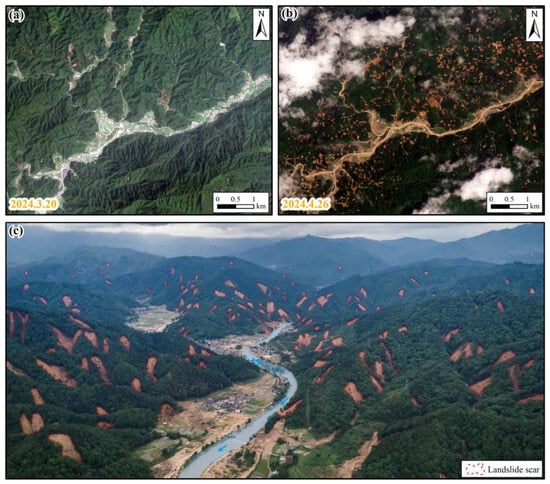
Figure 1.
Satellite and drone imagery before and after the rainfall event: (a) Pre-event Planet satellite image; (b) Post-event Planet satellite image; (c) Post-disaster drone imagery (image source: Guangdong Provincial Emergency Management Department []. Reprinted/adapted with permission from Ref. []. Copyright 2025, Springer Nature).
Optical remote sensing has become a key technology for landslide monitoring due to its wide spatial coverage, high resolution, and multi-temporal observation capabilities. Common landslide identification methods include image differencing [,], vegetation index differencing (e.g., Normalized Difference Vegetation Index, NDVI) [,,], spectral feature classification [], deep learning techniques [,,], and digital elevation model (DEM) analysis []. Among these, NDVI differencing efficiently detects vegetation loss in landslide areas through pre- and post-event comparisons. Its operational simplicity, low cost, and effectiveness in vegetated mountainous terrain make it particularly suitable for rapid identification. Unlike deep learning approaches requiring extensive labeled data and computational resources, NDVI differencing offers practical advantages for resource-constrained environments and time-sensitive post-disaster scenarios. Previous studies have successfully applied NDVI time-series analysis with automated thresholding and morphological processing for real-time landslide monitoring [,], especially after seismic events.
Landslide susceptibility mapping (LSM) is a crucial component of landslide disaster prevention and mitigation—typically integrates qualitative and quantitative approaches. Qualitative methods relying on expert knowledge and field surveys suffer from subjectivity and limited quantifiability. Quantitative approaches statistically model relationships between landslides and environmental factors using machine learning algorithms. Advances in Geographic Information Systems (GIS), remote sensing technologies, and computing power have enabled widespread adoption of machine learning models including Logistic Regression (LR) [,], Artificial Neural Networks (ANN) [], Support Vector Machines (SVM) [], Bayesian Algorithms [], Random Forests (RF) [], Extreme Gradient Boosting (XGBoost) [], and ensemble methods []. Deep learning models like Convolutional Neural Networks (CNNs) [,] also show promising accuracy and generalizability. However, model performance varies significantly across geological settings and landslide types [,,,,], with no universally optimal single model. Comparative multi-model evaluation combined with explainable AI techniques (e.g., SHAP—Shapley Additive Explanations) is therefore essential for enhancing model selection rigor and interpretability [].
In this study, we focus on the large-scale landslide disaster induced by the extreme rainfall event in Jiangwan Town, Shaoguan City, in April 2024. The main objectives are: (1) Implement rapid landslide identification using NDVI differencing to establish a comprehensive event inventory; (2) Analyze spatial distribution patterns and controlling mechanisms by integrating topographic, pedological, and meteorological factors; (3) Evaluate predictive performance of multiple machine learning models and identify dominant landslide drivers through SHAP analysis. The findings provide technical support for rapid risk assessment of extreme-rainfall-induced landslides in the study area, while offering methodological references for emergency response and mitigation strategies in similar mountainous regions.
2. Background
2.1. Study Area
Jiangwan Town is located in the southwest of Wujiang District, Shaoguan City, Guangdong Province, southern China (113°7′E–113°20′E and 24°32′N–24°50′N), situated in the southern section of the Nanling Mountains. It borders Qujiang District to the east and Ruyuan Yao Autonomous County to the west (Figure 2b). The elevation in the study area ranges from 116 to 1357 m, and the topography is predominantly characterized by low mountains and hills (Figure 2c). Jiangwan Town is characterized by a subtropical monsoon climate, with an average annual precipitation of about 1500 mm, mainly concentrated in April to August, which is also the period of high incidence of rainfall-induced natural hazards [].
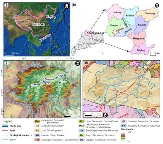
Figure 2.
Topographic and geological condition of the study area: (a) Location of Guangdong Province in China; (b) Location of Jiangwan Town within Shaoguan City; (c) Topographic map; (d) Geological map (Data source: 1:20,000 Digital Geological Map Spatial Database of China []).
Based on the 1:20,000 Digital Geological Map Spatial Database of China [], we mapped the stratigraphic distribution within the study area (Figure 2d). The main exposed strata include: the Devonian Laohutou Formation (Dl), primarily composed of conglomeratic sandstone and sparsely distributed in the southern and northern parts of the study area; the Devonian Yangxi Formation (Dy), dominated by conglomerate and occurring in limited areas in the north; the Early Jurassic granite (J1γ), consisting mainly of biotite granite and widely distributed across the region; and the Late Jurassic granite (J3γ), which is sporadically distributed in the eastern, western, and northern parts of the study area.
2.2. The Rainstorm Event
According to data from the Shaoguan Station of the National Meteorological Data Center, Shaoguan City has experienced multiple torrential rainfall events since April 2024. The monthly cumulative precipitation reached 975 mm (Figure 3a), significantly exceeding the historical average of 129.9 mm for the same period and breaking the previous record of 477.3 mm set in 1951 [].
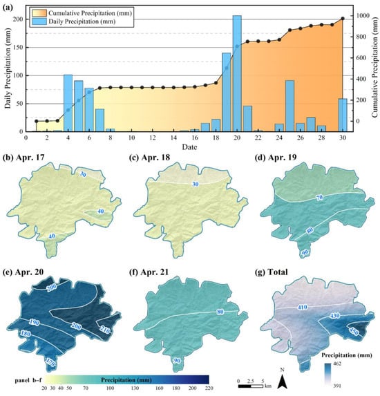
Figure 3.
Characteristics of April 2024 rainfall in the study area: (a) Monthly rainfall recorded at the Shaoguan meteorological station; (b–f) Daily rainfall distribution in Jiangwan Town from 17 to 21 April; (g) Cumulative rainfall distribution in Jiangwan Town from 17 to 21 April.
Particularly between 17 and 21 April, daily precipitation ranged from 15.2 mm to 206 mm (recorded on 20 April), with a five-day cumulative rainfall of 430 mm. This extreme event induced clusters of landslides across the region.
To comprehensively characterize the rainfall distribution across the study area, we performed Inverse Distance Weighting (IDW) interpolation using precipitation data from seven adjacent national-level meteorological stations: Shaoguan, Chenzhou, Lianzhou, Fogang, Lianping, Xunwu, and Ganzhou. The resulting spatial distribution map of the five-day cumulative rainfall is presented in Figure 3g.
3. Data and Methods
3.1. Data
We collected and processed multiple spatial datasets for landslide inventory mapping and obtaining factors that construct landslide susceptibility. The primary data sources include optical satellite imagery, DEM, river networks, lithology, and precipitation data, with detailed specifications provided in Table 1.

Table 1.
Data used in this study.
To ensure consistency in spatial analysis, all raster datasets were resampled to a 30 m resolution and projected into the WGS_1984_UTM_Zone_49N coordinate system. Topographic factors—including slope, aspect, curvature, topographic wetness index (TWI), and topographic relief—were derived from the 30 m-resolution Copernicus DEM using GIS-based terrain analysis tools (ArcGIS (v10.8)). The distance from rivers was calculated by generating multi-ring buffers from river vector data and subsequently converting these buffers to raster format. Additionally, lithology and rainfall data were incorporated as importance influencing factors in the LSM.
3.2. Landslide Mapping and Validation
Jiangwan Town exhibits dense vegetation coverage, where landslide disasters have inflicted severe damage to local vegetation. The NDVI, a key parameter reflecting vegetation coverage status, is widely employed in environmental monitoring and natural hazard studies due to its sensitivity to surface changes []. To ensure the accuracy of NDVI calculations, PlanetScope images acquired during pre- and post-rainfall events underwent comprehensive preprocessing, including radiometric calibration, atmospheric correction, and geometric rectification. Following preprocessing, NDVI was calculated for the respective images (Figure 4a,b) using the formula below []:
where and denote the reflectance values in the near-infrared and red spectral bands, respectively.
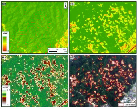
Figure 4.
Workflow of the NDVI difference-based landslide detection method: (a) Pre-event NDVI; (b) Post-event NDVI; (c) Landslide extraction based on NDVI differences (white boundaries represent landslide areas identified using a threshold of −0.6 to −0.1); (d) Final landslide boundaries after manual correction.
To quantify vegetation changes, the NDVI difference (ΔNDVI) between the two images was calculated using the following formula:
where NDVIpre and NDVIpost represent the NDVI values before and after the rainfall event, respectively.
We plotted the density distribution of ΔNDVI values for both landslide areas and non-landslide areas (Figure 5). The range of −0.6 < ΔNDVI < −0.1 was found to encompass the majority of landslide occurrences, and thus was selected as the optimal threshold interval for automated landslide extraction (Figure 4c). However, unavoidable environmental noise—such as bare soil, water bodies, and shadows []—significantly interfered with the extraction accuracy, resulting in commission and omission errors.
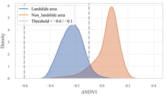
Figure 5.
Density distribution of ΔNDVI values for landslide areas and non-landslide areas.
Furthermore, the landslide boundaries extracted solely based on the ΔNDVI threshold did not consider topographic effects, occasionally causing adjacent landslide patches to be over-aggregated into single connected features. To improve the accuracy of the landslide mapping results, post-processing and manual refinement were applied to the initial automated output. The post-processing comprised three key steps:
- (1)
- Slope Constraint: Incorporating terrain factors, a slope threshold (>5°) applied to exclude misclassified areas in flat or anomalous terrain.
- (2)
- Area Threshold Filtering: Isolated noise patches smaller than the minimum expected landslide area (100 m2) were removed.
- (3)
- Morphological Operations: Erosion and dilation operations were performed to:
- Enhance boundary delineation.
- Fill holes within pixel-dense regions.
- Improve the spatial coherence and geometric integrity of landslide patches.
Following this post-processing sequence, a refined landslide distribution map was generated (Figure 4d).
Based on the landslide inventory provided by Fang et al. (2024) [], we validated our landslide mapping results (Figure 6), which demonstrated high reliability. To further evaluate the accuracy of the landslide extraction results derived using the NDVI differencing method, a pixel-level comparison was performed using the inventory from Fang et al. (2024) [] as the reference dataset. The corresponding confusion matrix is presented below:
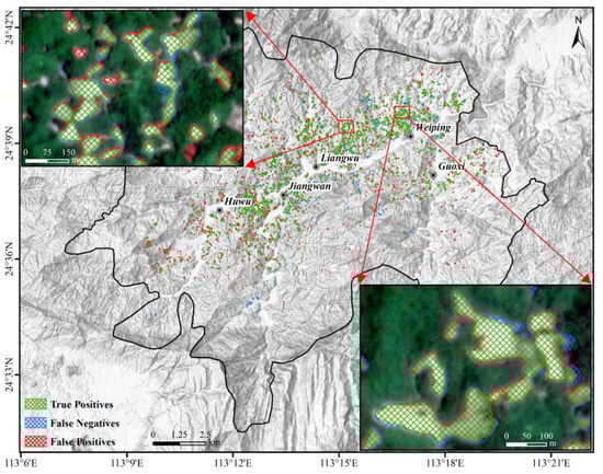
Figure 6.
Validation of landslide mapping results using the reference inventory.
Based on the matrix, the overall accuracy (OA) was calculated as 99.15%, with a Kappa coefficient of 0.82. These metrics indicate substantial consistency between the automated extraction results and the manual interpretation. Furthermore, the precision and recall rates were 78.99% and 85.32%, respectively.
3.3. Landslide Distribution Pattern Analysis
To investigate the relationship between rainfall-induced landslide distribution and influencing factors, we employ two widely used metrics: Landslide Number Density (LND) and Landslide Area Density (LAD) [,]. LND quantifies the number of landslides per square kilometer (Equation (3)), while LAD represents the percentage of landslide area within each factor category (Equation (4)).
The combination of LND and LAD values offers a nuanced understanding of landslide characteristics. For example, a high LND but low LAD suggests the predominance of small-scale landslides, whereas a low LND with high LAD indicates fewer but larger landslides. When both LND and LAD are high, it implies a severely affected area with widespread and extensive landslide activity, necessitating further evaluation based on both the number and scale of landslides.
The combined interpretation of LND and LAD values reveals distinct patterns in landslide characteristics. A high LND coupled with a low LAD denotes frequent occurrences of small-scale landslides. Conversely, a low LND alongside a high LAD suggests a landscape dominated by large-scale landslide events. Where both metrics exhibit high values, this reflects severe landslide development; such scenarios necessitate comprehensive evaluation incorporating total landslide inventory data to accurately assess hazard intensity.
3.4. Landslide Susceptibility Modeling
3.4.1. Conditioning Factors
Based on the spatial distribution patterns and formation conditions of landslides within the study area, and referencing environmental factors from regions with similar geomorphic characteristics, we selected ten fundamental environmental conditioning factors: elevation, slope, aspect, plane curvature, profile curvature, topographic relief, TWI, precipitation, lithology, and distance from the river (Figure 7).
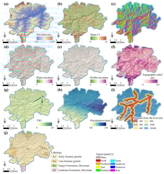
Figure 7.
Factors for LSM: (a) Elevation; (b) Slope; (c) Aspect; (d) Plane curvature; (e) Profile curvature; (f) Topographic relief; (g) TWI; (h) Precipitation; (i) Distance from the river; (j) Lithology.
3.4.2. Mapping Units
Slope units, grid cells, and terrain units are commonly used as evaluation units in LSM. The selection of evaluation unit significantly influences the accuracy of LSM []. Among these, grid cells are the most prevalent; however, their geometric configuration often fails to align with the actual geomorphological features controlling landslide occurrence, limiting their ability to precisely predict landslide locations or adequately represent topographic characteristics of landslide-prone areas.
In contrast, slope units better correspond to landslide morphological features and more accurately reflect terrain attributes. Consequently, slope units offer distinct advantages for LSM. Traditional extraction methods for slope units predominantly rely on hydrological analysis, yet this approach often neglects the homogeneity assumption critical for landslide stability analysis. Additionally, these methods require manual correction, are time-consuming, and prove impractical for large-scale studies [].
This study employed the slopeunits module in GRASS GIS (v7.8) to extract slope units from DEM data. Through iterative parameter optimization, we derived a dataset comprising 2826 slope units, thereby establishing a more precise mapping framework for subsequent LSM.
3.4.3. Modeling Approach
To mitigate uncertainties arising from model selection in rainfall-induced LSM [], we employed multiple machine learning algorithms, including LR, SVM, RF, and XGBoost.
- (1)
- LR
Logistic regression is a nonlinear regression model accommodating both continuous and discrete independent variables, with a binary categorical dependent variable. The model employs maximum likelihood estimation to determine weights for environmental factors []. Its algorithm is expressed in Equations (5) and (6):
where p denotes the probability of landslide occurrence (ranging between 0 and 1), Z is the weighted sum of variables, xn represent environmental factors, bn are regression coefficients, and a is a constant term.
- (2)
- Support Vector Machine (SVM)
The Support Vector Machine algorithm operates by nonlinearly transforming input variables into a high-dimensional feature space, where it constructs an optimal decision function. This approach employs kernel functions in the original space to replace complex dot-product operations within the transformed feature space. Through training on finite samples, SVM achieves a globally optimal solution [,]. Given a training set , the separating hyperplane can be expressed by Equation (7):
where xi represents the input vector and yi denotes the output value, d signifies the feature dimension of the samples, and n indicates the total number of training samples. The parameters w and b correspond to the normal vector and the intercept of the hyperplane, respectively. Since estimation errors may prevent all data points from strictly satisfying the margin constraints, slack variables () are introduced. This transforms the problem into the following optimization framework, characterized by the objective function and constraints given in Equations (8)–(10):
In Equation (8), C denotes the penalty coefficient, which balances the accuracy of the linear fit against estimation errors. The choice of kernel function significantly influences the prediction outcomes. To achieve relatively low bias and favorable learning performance, the radial basis function (RBF) kernel was adopted in this study.
where is the characteristic dimension of the data sample.
- (3)
- RF
The Random Forest model, an ensemble learning method comprising multiple decision trees, operates on the principle where each node votes on input variables to determine the optimal classification outcome [,]. The implementation involves: (1) Bootstrap sampling, where multiple samples are drawn with replacement from the original training dataset, each retaining the original dataset size; (2) Decision tree construction, wherein each tree is grown using a Bootstrap sample, and at each node, a random subset of features is selected as candidates for splitting, with the optimal feature chosen for node partitioning; and (3) Ensemble prediction, where final classifications for new instances are determined by majority voting across all trees. To optimize predictive performance, hyperparameter tuning was performed, with the final adopted optimal parameters detailed in Table 2.
- (4)
- XGBoost
Table 2.
Hyperparameter Settings for RF and XGBoost models.
XGBoost, a scalable tree boosting machine learning system proposed by Chen and Guestrin in 2016 [], represents one of the most widely adopted regression algorithms due to its high predictive accuracy. Key advantages include parallel computation capabilities, optimized memory utilization, and efficient handling of sparse data. Compared to linear models, XGBoost typically delivers superior accuracy, particularly when processing complex datasets. However, this enhanced performance comes at the cost of interpretability, as understanding the internal decision mechanisms proves more challenging than in linear models. Hyperparameter tuning was similarly applied to the XGBoost model, with the final optimized parameter configuration detailed in Table 2.
4. Results
4.1. Landslide Inventory
We employed the NDVI differential method to identify rainfall-induced landslides. Pre-event imagery (20 March 2024) and post-event imagery (26 April and 14 May 2024) were processed for automated landslide extraction, followed by manual verification. A total of 1426 landslides were identified, covering a cumulative area of 4.56 km2. The largest single landslide spanned 0.11 km2, while the average landslide area was 3118 m2 (Figure 8). Approximately 84.3% of landslides exhibited areas below 5000 m2. These landslides demonstrated distinct linear clustering along both sides of Weiping Village, Liangwu Village, and Jiangwan Community.
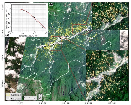
Figure 8.
Inventory of landslides induced by the 20 April 2024 extreme rainfall event in Jiangwan Town: (a) PDF of landslide areas fitted by the inverse gamma distribution; (b) Spatial distribution of landslides.
Landslide number density analysis using a 500 m search radius revealed a peak density value of 62.8 landslides/km2. Geographically, landslides concentrated primarily in the northeastern and central sectors of the study area (Figure 9).
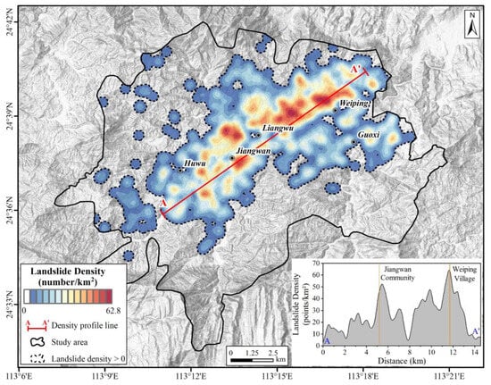
Figure 9.
Spatial distribution of landslide density.
The inventory is dominated by small-to-medium scale landslides with pronounced clustering characteristics, while large-scale landslides were infrequent. Fitting the landslide area probability density function (PDF) with an inverse gamma distribution [,] (Figure 8a) indicated general conformity to this distribution. A characteristic turning point delineates landslides of different scales. Further analysis demonstrated that the large-scale segment follows a power-law decay pattern, wherein probability density decreases with increasing landslide area [].
4.2. Characteristics of Landslide Development
4.2.1. Elevation
Statistical analysis indicates that majority of landslides occurred within the elevation range of 200–600 m. This range was further divided into six intervals with 100 m increments. Both LND and LAD exhibit a pattern of initial increase followed by a decrease, with peak values observed in the 200–300 m interval, reaching 17.04 km−2 and 5.80%, respectively. Within this elevation interval, both the number of landslides (totaling 646) and the cumulative landslide area were the highest, indicating that landslides are primarily concentrated in the 200–300 m elevation zone (Figure 10b).
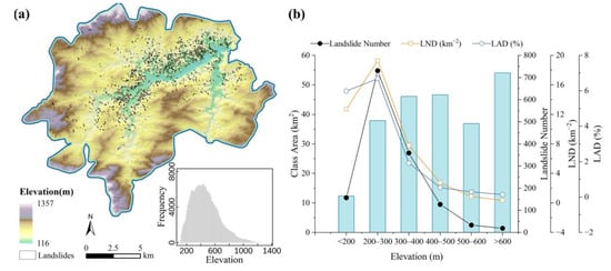
Figure 10.
Relationship between elevation and landslide distribution: (a) Elevation distribution in the study area; (b) Statistical analysis of LND and LAD.
4.2.2. Slope
As slope increases, the number of landslides, LND, and LAD all exhibited a trend of initial increase followed by subsequent decrease (Figure 11b). The peak values for all three indicators occur within the 20–30° slope range. In this interval, a total of 555 landslides were recorded, accounting for 44.51% of total the number of landslides; the LND reached 6.15 km−2, and the LAD reached 1.77%. These findings indicate that slopes ranging from 20° to 30° in Jiangwan Town are the most susceptible to landslide occurrences.
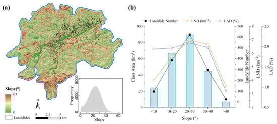
Figure 11.
Relationship between slope and landslide distribution: (a) Slope distribution in the study area; (b) Statistical analysis of LND and LAD.
4.2.3. Aspect
Landslide distribution across aspect shows limited variation in quantity. Relatively concentrated occurrences are observed on north (N), northwest (NW), south (S), and southeast (SE) aspects, while the remaining four aspects exhibit sparser distributions. In terms of areal distribution within the Jiangwan study area, landslides predominantly cluster on north, south, and southeast-facing slopes. Notably, higher values of both LND and LAD are recorded on west (W), southwest (SW), and northwest (NW) aspects (Figure 12b). This indicates that slopes facing west, southwest, and northwest within the Jiangwan area exhibit the highest susceptibility to landslide occurrence.
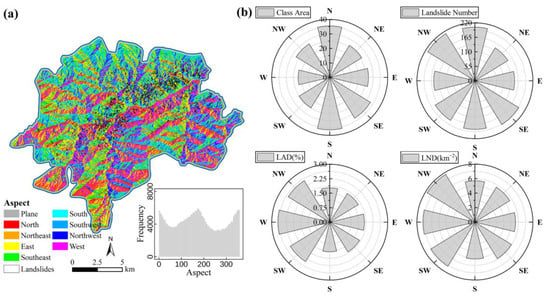
Figure 12.
Relationship between aspect and landslide distribution: (a) Aspect distribution in the study area; (b) Statistical analysis of LND and LAD.
4.2.4. Rainfall
Figure 13 presents the relationship between landslide distribution and rainfall on 20 April as well as the five-day cumulative rainfall from 17 to 21 April. The results show that when the single-day cumulative rainfall on 20 April was in the range of 190–200 mm, both the number of landslides, landslide number density (LND), and landslide area density (LAD) reached relatively high values, indicating that most landslides occurred within this rainfall range. For the five-day cumulative rainfall, the number of landslides, LND, and LAD were also significantly higher within the 400–410 mm, 410–420 mm, and 420–430 mm intervals, suggesting that landslides were more likely to occur in areas where total rainfall over five days ranged from 400 to 430 mm. In terms of spatial distribution, the five-day cumulative rainfall primarily determined the spatial extent of landslide occurrence and the accumulation of soil moisture, while the short-duration intense rainfall on 20 April played a more direct role in triggering landslides. This indicates that short-term heavy rainfall is the primary driving factor for landslide initiation.
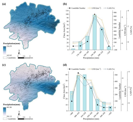
Figure 13.
Relationship between precipitation and landslide distribution: (a) Relationship between precipitation on 20 April 2024; (b) Statistical analysis of LND and LAD for precipitation on 20 April 2024; (c) Relationship between five-day cumulative precipitation; (d) Statistical analysis of LND and LAD for five-day cumulative precipitation.
4.3. Landslide Susceptibility Mapping
Prior to modeling, correlation analysis was performed among the environmental factors to ensure their relative independence and mitigate potential accuracy issues arising from multicollinearity []. The correlation coefficients calculated between the ten initial environmental factors revealed strong correlations between plane curvature and both the TWI and profile curvature. Consequently, plane curvature was excluded from the subsequent LSM. The correlation coefficients among the remaining nine factors were all below 0.6 (Figure 14), indicating the absence of strong collinearity. These nine factors thus met the requirements for input variables in the landslide prediction model. It should be noted that rainfall interpolation utilized elevation as a covariate, resulting in observed correlations between the precipitation factor and both elevation and topographic relief.
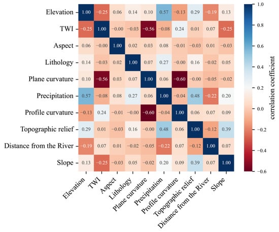
Figure 14.
Pearson correlation coefficients among evaluation factors.
Four machine learning models—LR, SVM, RF, and XGBoost—were evaluated using 10-fold cross-validation to compute landslide susceptibility index. These indices were classified into five levels (very low, low, medium, high, and very high) via natural break classification. The distribution of landslide counts and areal coverage across susceptibility zones is presented in Table 3, with spatial patterns illustrated in Figure 15.
Table 3.
Statistics of landslide susceptibility zonations for different models.
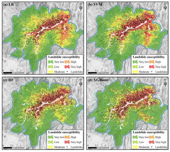
Figure 15.
Landslide susceptibility maps generated using four different models: (a) LR; (b) SVM; (c) RF; (d) XGBoost.
Regarding disaster occurrence, the four models classified 87.27% (LR), 85.15% (SVM), 81.75% (RF), and 75.81% (XGBoost) of disasters within medium–high susceptibility zones. In terms of spatial distribution, high susceptibility zones accounted for 21.03% (LR), 21.52% (SVM), 19.47% (RF), and 20.93% (XGBoost) of the total study area. Although variations exist in the precise area allocations and disaster counts across models, their spatial patterns for high susceptibility zones consistently converge. All models clearly identified concentrated high susceptibility along mountain slopes on both sides of river valleys, indicating these areas as primary landslide-prone regions.
The classification performance of the four models was evaluated using Receiver Operating Characteristic (ROC) curves [,] (Figure 16). The Area Under the Curve (AUC) statistic for each model was calculated through 10-fold cross-validation, with the results summarized in Figure 17.
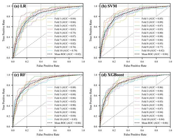
Figure 16.
ROC curves of four models: (a) LR; (b) SVM; (c) RF; (d) XGBoost. The grey dashed line represents the reference line of the ROC curve.
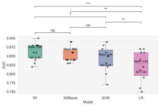
Figure 17.
Pairwise comparison of AUC values among four models using paired t-tests. Here, * indicates a significance level of p < 0.05, ** indicates p < 0.01, *** indicates p < 0.001, and ns indicates no significant difference (p ≥ 0.05).
RF demonstrated the highest maximum AUC (0.90), followed closely by XGBoost and SVM (both 0.89), while LR achieved the lowest maximum AUC (0.87). Regarding mean AUC, both XGBoost and RF attained the highest value (0.86), indicating superior overall classification capability. SVM yielded a mean AUC of 0.84, marginally lower than the top performers, whereas LR exhibited the weakest mean performance (AUC = 0.82). Model stability was further assessed by calculating the standard deviation (SD) of AUC values across folds. RF (SD = 0.03) and XGBoost (SD = 0.02) showed the most consistent performance, followed by SVM (SD = 0.04), and LR (SD = 0.04) displayed the highest variability, suggesting greater performance fluctuation.
No significant difference was observed between RF and XGBoost (p > 0.05), indicating comparable classification efficacy. However, RF significantly outperformed SVM (p < 0.05) and exhibited highly significant superiority over LR (p < 0.001). While XGBoost showed no significant advantage over SVM (p > 0.05), it significantly surpassed LR (p < 0.01). SVM also demonstrated significantly better performance than LR (p < 0.01).
In summary, RF and XGBoost emerged as the most effective models for LSM, with statistically equivalent performance. SVM ranked second, significantly outperforming LR, which demonstrated the weakest performance among all models.
5. Discussion
5.1. Interpretability of Machine Learning Models
To enhance the interpretability of the landslide susceptibility model, we employed the SHAP method, based on Shapley values derived from cooperative game theory. SHAP quantifies the contribution of each feature to the model’s predictive outcomes, thereby elucidating the model’s decision-making process. This approach facilitates an understanding of how environmental factors influence landslide risk []. It not only aids in identifying and analyzing key factors governing landslide occurrence but also provides a quantitative comparison of their relative importance.
Using the XGBoost model, we generated SHAP visualizations including beeswarm plots and feature contribution plots (Figure 18). The results demonstrate significant and patterned contributions from the selected environmental factors to landslide susceptibility results. For instance, rainfall and slope exhibit a positive correlation with SHAP values, while SHAP values show an increasing trend with decreasing TWI, indicating their substantial influence on landslide occurrence.
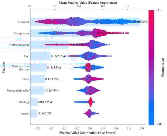
Figure 18.
SHAP visualization: hive plot and feature contribution plot.
The mean absolute SHAP values across all samples were calculated to generate a feature importance ranking plot, visually depicting the contribution magnitude of each factor. This plot reveals elevation, rainfall, profile curvature, and TWI as the top four contributing factors, all with mean SHAP values exceeding 0.2. Furthermore, distance to rivers, slope gradient, and topographic relief also show strong correlations with landslide occurrence, with mean SHAP values exceeding 0.1. In contrast, aspect and stratigraphy exhibit lower relevance and minimal impact.
5.2. Soil Moisture and Precipitation Response
Soil moisture plays a critical role in landslide initiation and triggering. Rainfall-induced saturation of shallow soils and elevated pore water pressure constitute a primary mechanism for slope destabilization [,,]. The spatiotemporal dynamics of soil moisture, particularly its delayed response following precipitation events, are essential for understanding landslide timing and early warning systems.
To investigate the relationship between precipitation and soil moisture, we utilized NASA’s Soil Moisture Active Passive (SMAP) satellite data from six monitoring sites in April 2024. Combining these measurements with synchronous precipitation records, we analyzed correlation patterns and lagged response characteristics (Figure 19). The SMAP dataset (0.25° resolution, daily scale) integrates ground observations, model simulations, and microwave remote sensing, offering exceptional spatiotemporal continuity for regional hydrological studies.
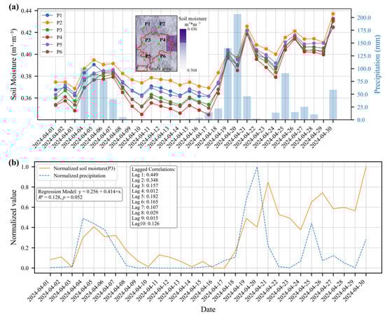
Figure 19.
Lagged correlation between soil moisture and precipitation: (a) Daily soil moisture time-series in April; (b) Temporal trend of lagged correlation between soil moisture and precipitation at P3.
Methodologically, soil moisture and precipitation data from site P3 underwent normalization (0–1 range) to eliminate scale effects. Correlation analysis revealed pronounced lagged responses, with peak correlation (r = 0.449) at 1-day lag—significantly higher than contemporaneous correlation (Lag 0: r = 0.128). This indicates maximum soil moisture sensitivity to antecedent precipitation. Linear regression further confirmed limited explanatory power under zero-lag conditions (R2 = 0.128, p = 0.052), underscoring the necessity of incorporating lag effects for model accuracy.
The SMAP data effectively captured regional moisture dynamics, demonstrating precipitation’s role as a key short-term driver. This temporal hysteresis reflects a hydrological “memory effect,” elucidating soil–water coupling mechanisms. However, despite the utility of SMAP data at the regional scale, its relatively coarse spatial resolution presents notable limitations when applied to heterogeneous terrain. In areas with complex topography—such as mountainous regions with variable slope gradients, land cover, and soil properties—a single SMAP grid cell may integrate highly diverse conditions, leading to spatial averaging and potential signal dilution. This mismatch between data resolution and topographic complexity may hinder accurate characterization of localized soil moisture variations critical for landslide prediction. To overcome this, future research should explore data fusion approaches, incorporating higher-resolution remote sensing products (e.g., Sentinel-1/2) and in situ observations to improve spatial representation of soil moisture dynamics in complex terrains. In landslide triggering, soil moisture accumulation often functions as a priming-trigger mechanism: intense/sustained rainfall induces shallow saturation and reduced shear strength, culminating in slope failure. Quantifying precipitation–soil moisture hysteresis thus advances both infiltration process understanding and early-warning parameterization.
Nevertheless, single-factor precipitation models exhibit inherent limitations in predicting soil moisture variation. Future research should incorporate multi-source environmental factors (e.g., slope gradient, vegetation cover, soil texture, land use, and evapotranspiration) through integrated remote sensing and field observations. Such holistic hydro-geological process modeling will enhance soil moisture dynamic interpretation and landslide trigger prediction, ultimately supporting landslide risk mitigation strategies.
6. Conclusions
During 17–21 April 2024, extreme rainfall in Shaoguan City, Guangdong Province (particularly in Jiangwan Town, Wujiang District) triggered numerous landslides. This study integrated optical remote sensing imagery with NDVI differencing to automatically extract rainfall-induced landslides, analyze their spatial distribution patterns and causative factors in Jiangwan Town, and evaluate four machine learning models for LSM. Key conclusions are as follows:
- (1)
- Employing NDVI differencing of pre- and post-rainfall imagery coupled with threshold segmentation enabled rapid automated extraction of landslides in Jiangwan Town, a total of 1426 landslides were identified, covering an aggregate area of 4.56 km2.
- (2)
- Landslides predominantly exhibited small-to-medium scales with significant clustering effects, forming a linear distribution pattern aligned northeast–southwest along river valleys. Spatial analysis revealed concentrated occurrences on slopes at 200–300 m elevation with 20–30° gradients.
- (3)
- Landslide susceptibility analysis using LR, SVM, RF, and XGBoost demonstrated superior classification performance for the RF and XGBoost models. High-susceptibility zones were primarily distributed on valley slopes. SHAP-based quantification identified elevation, precipitation, profile curvature, and topographic wetness index as dominant controlling factors.
Author Contributions
Conceptualization, R.W. and Y.S.; methodology, R.W., Y.S. and W.L.; software, Y.S., R.W. and L.W.; validation, Y.S. and D.P.; formal analysis, R.W., Y.S., G.H. and L.W.; investigation, R.W., G.Q., J.Q., G.H., L.F. and W.L.; resources, Y.S.; data curation, R.W., J.Q. and L.W.; writing—original draft preparation, R.W.; writing—review and editing, R.W. and Y.S.; visualization, R.W.; supervision, Y.S.; project administration, Y.S.; funding acquisition, R.W. and W.L. All authors have read and agreed to the published version of the manuscript.
Funding
This research was funded by Science and Technology Project of China Southern Power Grid (grant No. GDKJXM20230770), the Key Research and Development Program of Sichuan Province (grant No. 2023YFS0435), and the State Key Laboratory of Geohazard Prevention and Geoenvironment Protection Independent Research Project (grant No. SKLGP2022Z007).
Data Availability Statement
All data and results of this study are available from the corresponding author upon request.
Acknowledgments
Thanks to Planet Labs for providing the PlanetScope imagery data.
Conflicts of Interest
Authors Ruizeng Wei, Lei Wang, and Dawei Peng are employed by the Guangdong Key Laboratory of Electric Power Equipment Reliability, Electric Power Research Institute of Guangdong Power Grid Co., Ltd., a subsidiary of China Southern Power Grid. The funder had no role in the study design, data collection, analysis, decision to publish, or preparation of the manuscript. The remaining authors declare that the research was conducted in the absence of any commercial or financial relationships that could be construed as potential conflicts of interest.
References
- Xu, Q.; Xu, F.; Pu, C.; Li, W.; Fan, X.; Dong, X.; Wang, X.; Li, Z. Preliminary Analysis of Extreme Rainfall-Induced Cluster Landslides in Jiangwan Township, Shaoguan, Guangdong, April 2024. Geomat. Inf. Sci. Wuhan Univ. (In Chinese). 2024, 49, 1264–1274. [Google Scholar] [CrossRef]
- Yang, G.; Zhao, L.; Qin, Y.; Yang, T.; Chen, S. Clustered landslides induced by rainfall in Jiangwan Town, Shaoguan City, Guangdong Province, China. Landslides 2025, 22, 1325–1338. [Google Scholar] [CrossRef]
- Chen, L.; Xiang, X.; Wen, H.; Xiao, J.; Song, C.; Zhou, X.; Yu, J. Improve unsupervised Learning-based landslides detection by band ratio processing of RGB optical images: A case study on rainfall-induced landslide clusters. Geomat. Nat. Hazards Risk 2024, 15, 2363406. [Google Scholar] [CrossRef]
- Kovács, I.P.; Tessari, G.; Ogushi, F.; Riccardi, P.; Ronczyk, L.; Kovács, D.M.; Lóczy, D.; Pasquali, P. Do We Need a Higher Resolution? Case Study: Sentinel-1-Based Change Detection of the 2018 Hokkaido Landslides, Japan. Remote Sens. 2022, 14, 1350. [Google Scholar] [CrossRef]
- Aman, M.A.; Chu, H.-J.; Yunus, A.P. Exploration of Multi-Decadal Landslide Frequency and Vegetation Recovery Conditions Using Remote-Sensing Big Data. Earth Syst. Environ. 2025, 9, 197–213. [Google Scholar] [CrossRef]
- Notti, D.; Cignetti, M.; Godone, D.; Cardone, D.; Giordan, D. The unsuPervised shAllow laNdslide rapiD mApping: PANDA method applied to severe rainfalls in northeastern appenine (Italy). Int. J. Appl. Earth Obs. Geoinf. 2024, 129, 103806. [Google Scholar] [CrossRef]
- Wang, H.; Fan, S.; Huang, X.; Qiu, P.; Yu, J.; Li, J. Research on Real-Time Automatic Landslide Recognition Technology Based on Optical Image. Spacecr. Recovery Remote Sens. 2024, 45, 147–160. (In Chinese) [Google Scholar] [CrossRef]
- Yang, M.; Li, S.; Feng, Z. Post-seismic landslide extraction by combining texture analysis and emissivity estimating. Natl. Remote Sens. Bull. 2018, 22, 212–223. (In Chinese) [Google Scholar]
- Mohan, A.; Singh, A.K.; Kumar, B.; Dwivedi, R. Review on remote sensing methods for landslide detection using machine and deep learning. Trans. Emerging Telecommun. Technol. 2021, 32, e3998. [Google Scholar] [CrossRef]
- Yang, Z.; Qi, W.; Xu, C.; Shao, X. Exploring deep learning for landslide mapping: A comprehensive review. China Geol. 2024, 7, 330–350. [Google Scholar] [CrossRef]
- Chen, W.; Li, X.; Wang, Y.; Chen, G.; Liu, S. Forested landslide detection using LiDAR data and the random forest algorithm: A case study of the Three Gorges, China. Remote Sens. Environ. 2014, 152, 291–301. [Google Scholar] [CrossRef]
- Zhao, W.; Li, A.; Nan, X.; Zhang, Z.; Lei, G. Postearthquake Landslides Mapping From Landsat-8 Data for the 2015 Nepal Earthquake Using a Pixel-Based Change Detection Method. IEEE J. Sel. Top. Appl. Earth Obs. Remote Sens. 2017, 10, 1758–1768. [Google Scholar] [CrossRef]
- Sun, D.; Xu, J.; Wen, H.; Wang, D. Assessment of landslide susceptibility mapping based on Bayesian hyperparameter optimization: A comparison between logistic regression and random forest. Eng. Geol. 2021, 281, 105972. [Google Scholar] [CrossRef]
- Goyes-Peñafiel, P.; Hernandez-Rojas, A. Landslide susceptibility index based on the integration of logistic regression and weights of evidence: A case study in Popayan, Colombia. Eng. Geol. 2021, 280, 105958. [Google Scholar] [CrossRef]
- Selamat, S.N.; Abd Majid, N.; Taha, M.R.; Osman, A. Landslide Susceptibility Model Using Artificial Neural Network (ANN) Approach in Langat River Basin, Selangor, Malaysia. Land 2022, 11, 833. [Google Scholar] [CrossRef]
- Huang, F.; Zhang, J.; Zhou, C.; Wang, Y.; Huang, J.; Zhu, L. A deep learning algorithm using a fully connected sparse autoencoder neural network for landslide susceptibility prediction. Landslides 2020, 17, 217–229. [Google Scholar] [CrossRef]
- Sun, D.; Wen, H.; Wang, D.; Xu, J. A random forest model of landslide susceptibility mapping based on hyperparameter optimization using Bayes algorithm. Geomorphology 2020, 362, 107201. [Google Scholar] [CrossRef]
- Shan, Y.; Xu, Z.; Zhou, S.; Lu, H.; Yu, W.; Li, Z.; Cao, X.; Li, P.; Li, W. Landslide Hazard Assessment Combined with InSAR Deformation: A Case Study in the Zagunao River Basin, Sichuan Province, Southwestern China. Remote Sens. 2024, 16, 99. [Google Scholar] [CrossRef]
- Kavzoglu, T.; Teke, A. Predictive Performances of Ensemble Machine Learning Algorithms in Landslide Susceptibility Mapping Using Random Forest, Extreme Gradient Boosting (XGBoost) and Natural Gradient Boosting (NGBoost). Arab. J. Sci. Eng. 2022, 47, 7367–7385. [Google Scholar] [CrossRef]
- Pham, B.T.; Nguyen-Thoi, T.; Qi, C.; Phong, T.V.; Dou, J.; Ho, L.S.; Le, H.V.; Prakash, I. Coupling RBF neural network with ensemble learning techniques for landslide susceptibility mapping. Catena 2020, 195, 104805. [Google Scholar] [CrossRef]
- Wang, H.; Zhang, L.; Luo, H.; He, J.; Cheung, R.W.M. AI-powered landslide susceptibility assessment in Hong Kong. Eng. Geol. 2021, 288, 106103. [Google Scholar] [CrossRef]
- Hakim, W.L.; Rezaie, F.; Nur, A.S.; Panahi, M.; Khosravi, K.; Lee, C.-W.; Lee, S. Convolutional neural network (CNN) with metaheuristic optimization algorithms for landslide susceptibility mapping in Icheon, South Korea. J. Environ. Manag. 2022, 305, 114367. [Google Scholar] [CrossRef]
- Shang, H.; Su, L.; Liu, Y.; Tsangaratos, P.; Ilia, I.; Chen, W.; Cui, S.; Duan, Z. Assessment of the effects of characterization methods selection on the landslide susceptibility: A comparison between logistic regression (LR), naive bayes (NB) and radial basis function network (RBF Network). Bull. Eng. Geol. Environ. 2025, 84, 134. [Google Scholar] [CrossRef]
- Reichenbach, P.; Rossi, M.; Malamud, B.D.; Mihir, M.; Guzzetti, F. A review of statistically-based landslide susceptibility models. Earth Sci. Rev. 2018, 180, 60–91. [Google Scholar] [CrossRef]
- Huang, F.; Mao, D.; Jiang, S.-H.; Zhou, C.; Fan, X.; Zeng, Z.; Catani, F.; Yu, C.; Chang, Z.; Huang, J.; et al. Uncertainties in landslide susceptibility prediction modeling: A review on the incompleteness of landslide inventory and its influence rules. Geosci. Front. 2024, 15, 101886. [Google Scholar] [CrossRef]
- Liu, X.; Shao, S.; Zhang, C.; Shao, S. Effect of different mapping units, spatial resolutions, and machine learning algorithms on landslide susceptibility mapping at the township scale. Environ. Earth Sci. 2025, 84, 138. [Google Scholar] [CrossRef]
- Mao, Y.; Li, Y.; Teng, F.; Sabonchi, A.K.S.; Azarafza, M.; Zhang, M. Utilizing Hybrid Machine Learning and Soft Computing Techniques for Landslide Susceptibility Mapping in a Drainage Basin. Water 2024, 16, 380. [Google Scholar] [CrossRef]
- Zhou, C.; Yin, K.; Cao, Y.; Ahmed, B.; Li, Y.; Catani, F.; Pourghasemi, H.R. Landslide susceptibility modeling applying machine learning methods: A case study from Longju in the Three Gorges Reservoir area, China. Comput. Geosci. 2018, 112, 23–37. [Google Scholar] [CrossRef]
- Liu, Y.; Huang, J.; Lin, W. Zoning strategies for ecological restoration in the karst region of Guangdong province, China: A perspective from the “social-ecological system”. Front. Environ. Sci. 2024, 12, 1369635. [Google Scholar] [CrossRef]
- Li, C.; Wang, X.; He, C.; Wu, X.; Kong, Z.; Li, X. China national digital geological map (public version at 1: 200,000 scale) spatial database. Geol. China 2019, 46, 1–10. [Google Scholar]
- Wu, J.; Zha, X.; Chen, S.; Mao, L.; Huang, B. Variations of Rainfall Erosivity of Different Magnitudes in Shaoguan from 1951 to 2018. J. Soil Water Conserv. 2021, 35, 21–26. (In Chinese) [Google Scholar] [CrossRef]
- Shan, Y.; Dai, X.; Li, W.; Yang, Z.; Wang, Y.; Qu, G.; Liu, W.; Ren, J.; Li, C.; Liang, S.; et al. Detecting Spatial-Temporal Changes of Urban Environment Quality by Remote Sensing-Based Ecological Indices: A Case Study in Panzhihua City, Sichuan Province, China. Remote Sens. 2022, 14, 4137. [Google Scholar] [CrossRef]
- Li, R.; Ye, S.; Bai, Z.; Nedzved, A.; Tuzikov, A. Moderate Red-Edge vegetation index for High-Resolution multispectral remote sensing images in urban areas. Ecol. Indic. 2024, 167, 112645. [Google Scholar] [CrossRef]
- Fang, C.; Fan, X.; Wang, X.; Nava, L.; Zhong, H.; Dong, X.; Qi, J.; Catani, F. A globally distributed dataset of coseismic landslide mapping via multi-source high-resolution remote sensing images. Earth Syst. Sci. Data 2024, 16, 4817–4842. [Google Scholar] [CrossRef]
- Ma, H.; Wang, F.; Fu, Z.; Feng, Y.; You, Q.; Li, S. Characterizing the clustered landslides triggered by extreme rainfall during the 2024 typhoon Gaemi in Zixing City, Hunan Province, China. Landslides 2025, 22, 2311–2329. [Google Scholar] [CrossRef]
- Li, C.; Zhang, J.; Gao, L.; Chen, X.; Ma, S.; Yuan, R. Spatial Clustering and distribution characteristics of large landslides in the Yalong River Basin, China. Geomorphology 2025, 475, 109667. [Google Scholar] [CrossRef]
- Sun, D.; Gu, Q.; Wen, H.; Xu, J.; Zhang, Y.; Shi, S.; Xue, M.; Zhou, X. Assessment of landslide susceptibility along mountain highways based on different machine learning algorithms and mapping units by hybrid factors screening and sample optimization. Gondwana Res. 2023, 123, 89–106. [Google Scholar] [CrossRef]
- Alvioli, M.; Guzzetti, F.; Marchesini, I. Parameter-free delineation of slope units and terrain subdivision of Italy. Geomorphology 2020, 358, 107124. [Google Scholar] [CrossRef]
- Zhang, W.; Gu, X.; Tang, L.; Yin, Y.; Liu, D.; Zhang, Y. Application of machine learning, deep learning and optimization algorithms in geoengineering and geoscience: Comprehensive review and future challenge. Gondwana Res. 2022, 109, 1–17. [Google Scholar] [CrossRef]
- Lombardo, L.; Mai, P.M. Presenting logistic regression-based landslide susceptibility results. Eng. Geol. 2018, 244, 14–24. [Google Scholar] [CrossRef]
- Chen, X.; Wang, Z.; Wu, J.; Chen, S.; Xu, H.; Sun, Z.; Yang, G.; Jiang, J.; Chen, J. Voltage Sag Source Identification Method Based on VMD and IAO-SVM. Guangdong Electr. Power 2023, 36, 59–67. (In Chinese) [Google Scholar] [CrossRef]
- Chauhan, V.K.; Dahiya, K.; Sharma, A. Problem formulations and solvers in linear SVM: A review. Artif. Intell. Rev. 2019, 52, 803–855. [Google Scholar] [CrossRef]
- Ali, J.; Khan, R.; Ahmad, N.; Maqsood, I. Random forests and decision trees. Int. J. Comput. Sci. Issues 2012, 9, 272. [Google Scholar]
- Yao, H.; Li, B.; Huang, Z. Small Signal Stability Assessment and Correction Control of Power System Based on Random Forest Algorithm. Guangdong Electr. Power 2023, 36, 60–69. (In Chinese) [Google Scholar] [CrossRef]
- Chen, T.; Guestrin, C. XGBoost: A Scalable Tree Boosting System. In Proceedings of the 22nd ACM SIGKDD International Conference on Knowledge Discovery and Data Mining, San Francisco, CA, USA, 13–17 August 2016; pp. 785–794. [Google Scholar]
- Qiu, H.; Hu, S.; Yang, D.; He, Y.; Pei, Y.; Kamp, U. Comparing landslide size probability distribution at the landscape scale (Loess Plateau and the Qinba Mountains, Central China) using double Pareto and inverse gamma. Bull. Eng. Geol. Environ. 2021, 80, 1035–1046. [Google Scholar] [CrossRef]
- Malamud, B.D.; Turcotte, D.L.; Guzzetti, F.; Reichenbach, P. Landslide inventories and their statistical properties. Earth Surf. Process. Landf. 2004, 29, 687–711. [Google Scholar] [CrossRef]
- Qiu, H.; Su, L.; Tang, B.; Yang, D.; Ullah, M.; Zhu, Y.; Kamp, U. The effect of location and geometric properties of landslides caused by rainstorms and earthquakes. Earth Surf. Process. Landf. 2024, 49, 2067–2079. [Google Scholar] [CrossRef]
- Lee, S.; Ryu, J.-H.; Kim, I.-S. Landslide susceptibility analysis and its verification using likelihood ratio, logistic regression, and artificial neural network models: Case study of Youngin, Korea. Landslides 2007, 4, 327–338. [Google Scholar] [CrossRef]
- Wei, A.; Ke, H.; He, S.; Jiang, M.; Yao, Z.; Yi, J. Enhanced Landslide Risk Evaluation in Hydroelectric Reservoir Zones Utilizing an Improved Random Forest Approach. Water 2025, 17, 946. [Google Scholar] [CrossRef]
- Ke, C.; Sun, P.; Zhang, S.; Li, R.; Sang, K. Influences of non-landslide sampling strategies on landslide susceptibility mapping: A case of Tianshui city, Northwest of China. Bull. Eng. Geol. Environ. 2025, 84, 123. [Google Scholar] [CrossRef]
- Zhang, J.; Ma, X.; Zhang, J.; Sun, D.; Zhou, X.; Mi, C.; Wen, H. Insights into geospatial heterogeneity of landslide susceptibility based on the SHAP-XGBoost model. J. Environ. Manag. 2023, 332, 117357. [Google Scholar] [CrossRef] [PubMed]
- Zhang, Z.; Zeng, R.; Meng, X.; Zhao, S.; Wang, S.; Ma, J.; Wang, H. Effects of changes in soil properties caused by progressive infiltration of rainwater on rainfall-induced landslides. Catena 2023, 233, 107475. [Google Scholar] [CrossRef]
- Liu, W.; Bai, R.; Sun, X.; Yang, F.; Zhai, W.; Su, X. Rainfall- and Irrigation-Induced Landslide Mechanisms in Loess Slopes: An Experimental Investigation in Lanzhou, China. Atmosphere 2024, 15, 162. [Google Scholar] [CrossRef]
Disclaimer/Publisher’s Note: The statements, opinions and data contained in all publications are solely those of the individual author(s) and contributor(s) and not of MDPI and/or the editor(s). MDPI and/or the editor(s) disclaim responsibility for any injury to people or property resulting from any ideas, methods, instructions or products referred to in the content. |
© 2025 by the authors. Licensee MDPI, Basel, Switzerland. This article is an open access article distributed under the terms and conditions of the Creative Commons Attribution (CC BY) license (https://creativecommons.org/licenses/by/4.0/).