
Simulation of Active Layer Thickness Based on Multi-Source Remote Sensing Data and Integrated Machine Learning Models: A Case Study of the Qinghai-Tibet Plateau

 ,
,  , ,
, ,  , and
, and
Abstract
1. Introduction
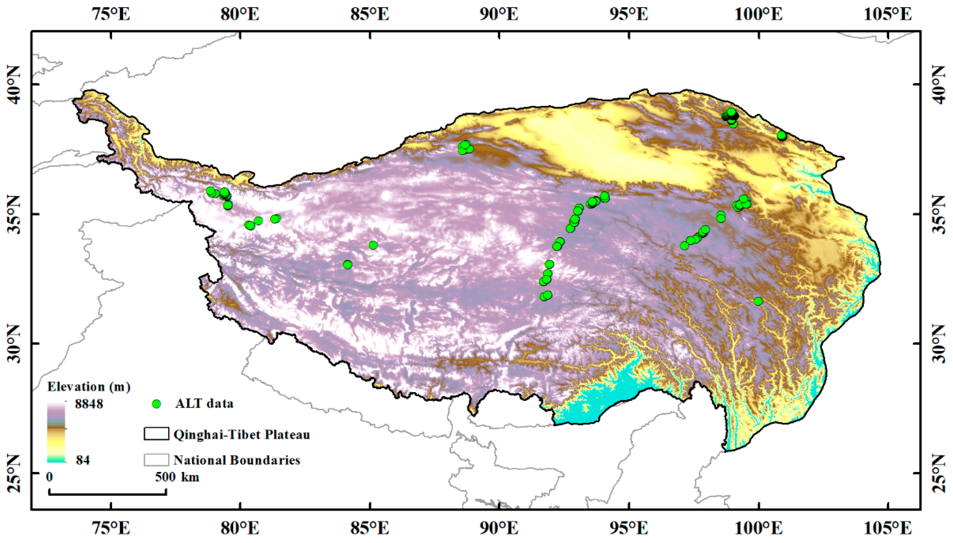
2. Study Area
3. Data and Method
3.1. Data
3.1.1. Remote Sensing Data and Meteorological Data
3.1.2. Active Layer Thickness (ALT) Data and Permafrost Data
3.1.3. Meteorological Station Data
3.2. Method
3.2.1. Extra Trees
3.2.2. CatBoost
3.2.3. Blending
3.3. Feature Selection
3.4. Stefan CatBoost-ET Model
3.5. Data Processing
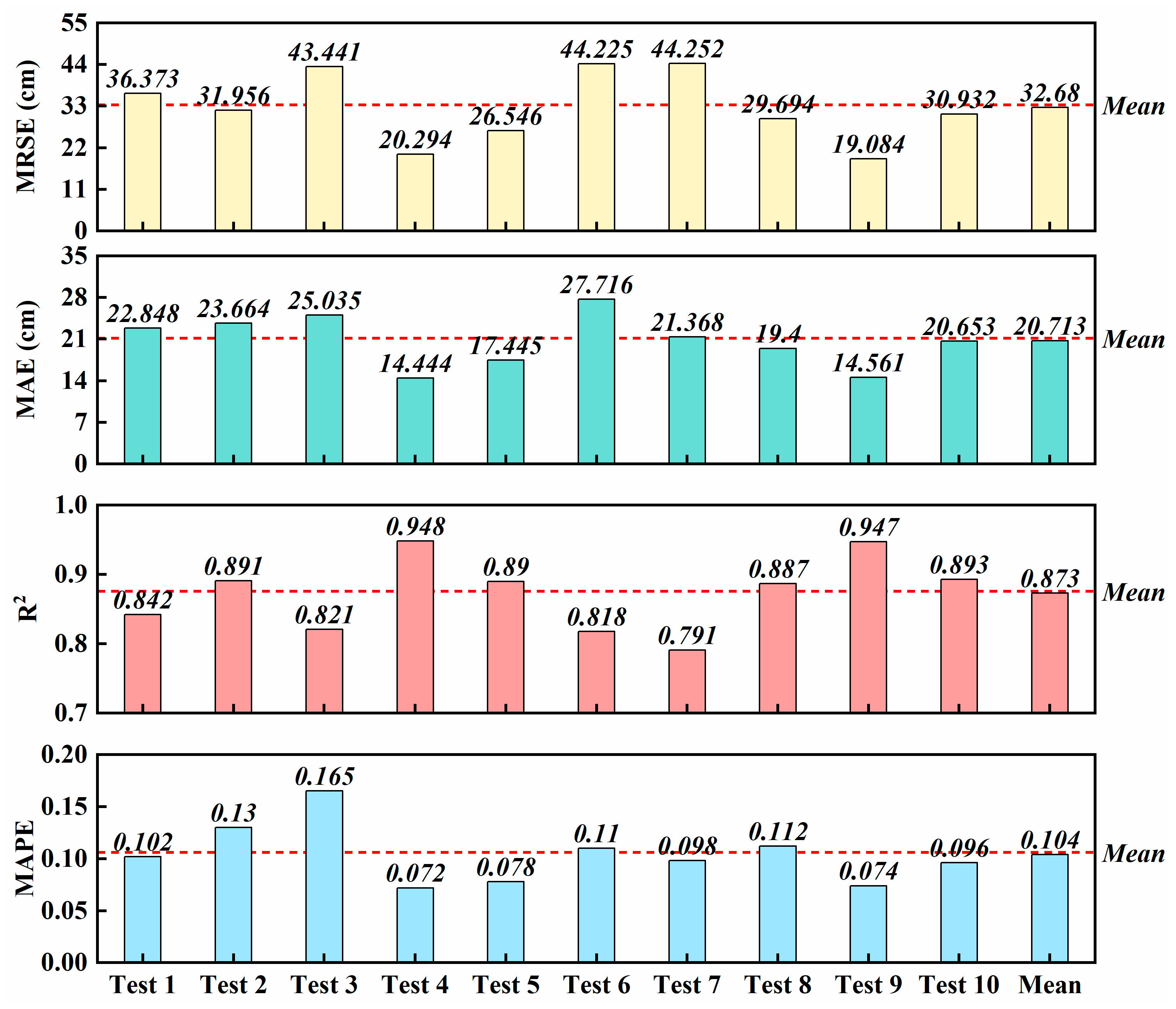
3.6. Model Accuracy Evaluation and Robustness Index
4. Result
4.1. ALT Simulation Results Using Multiple Machine Learning Models
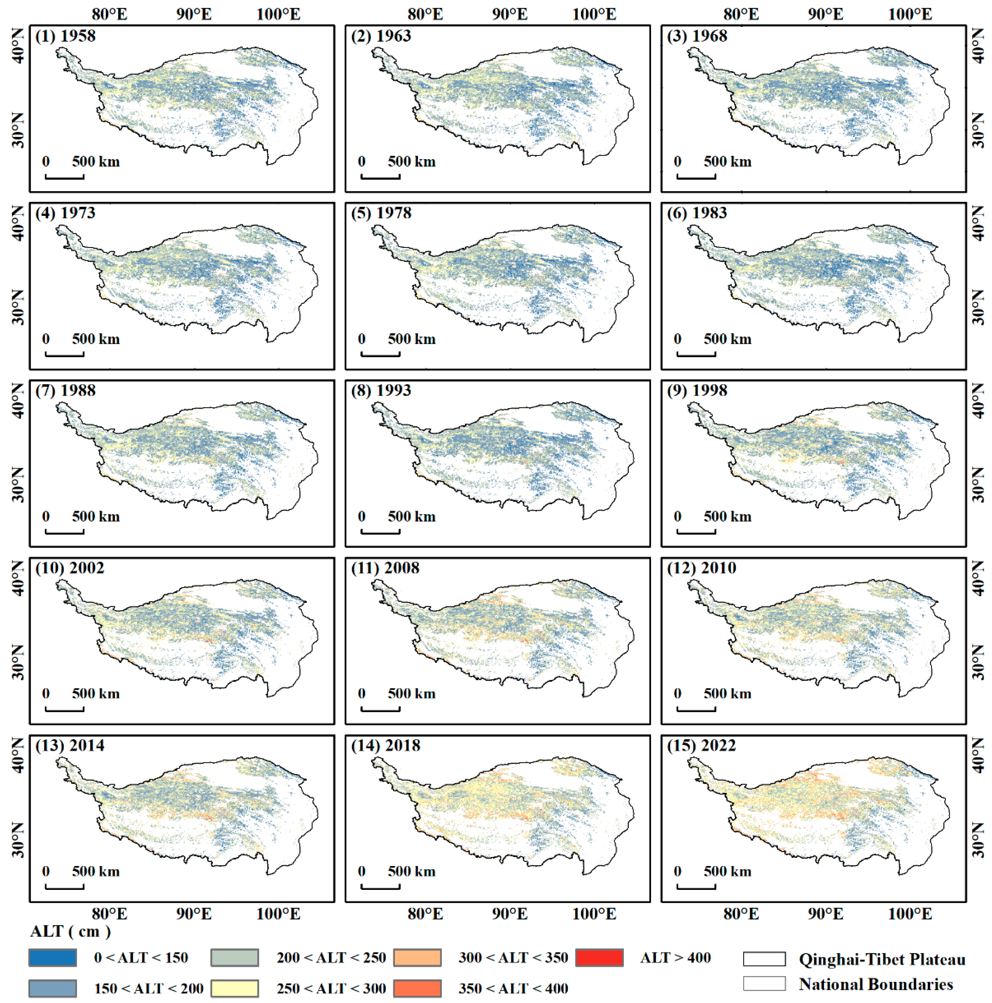
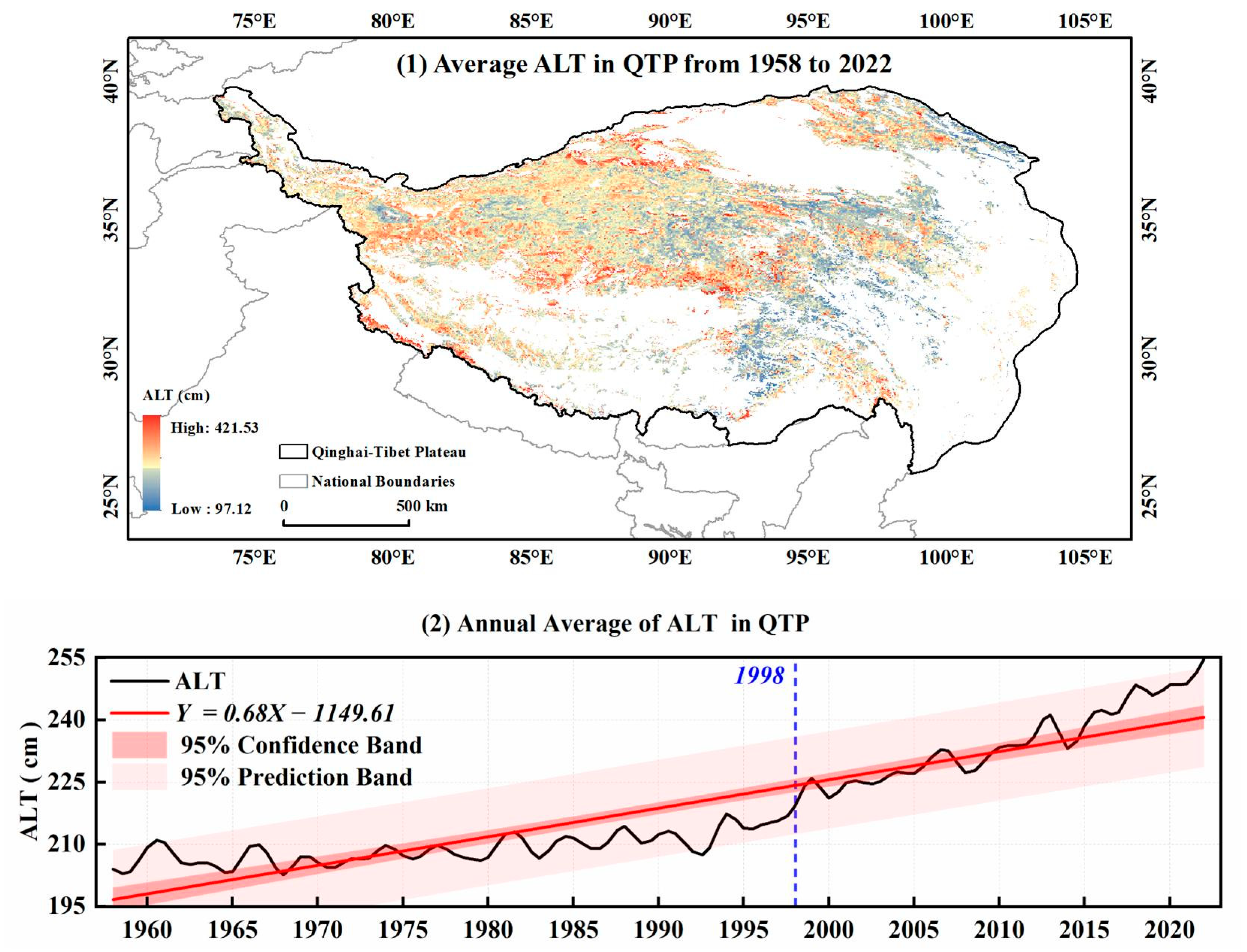
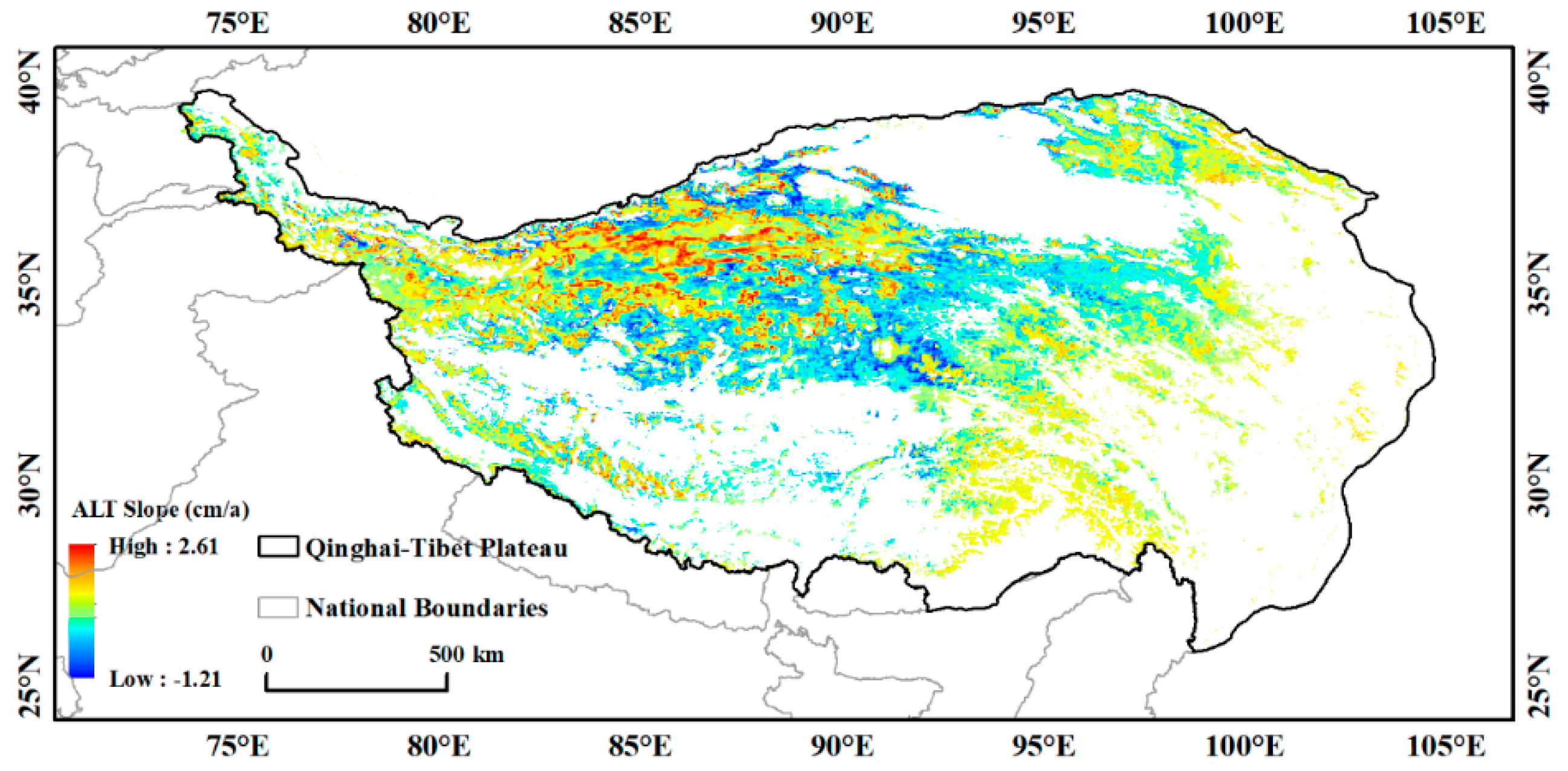
4.2. Analysis of ALT Changes
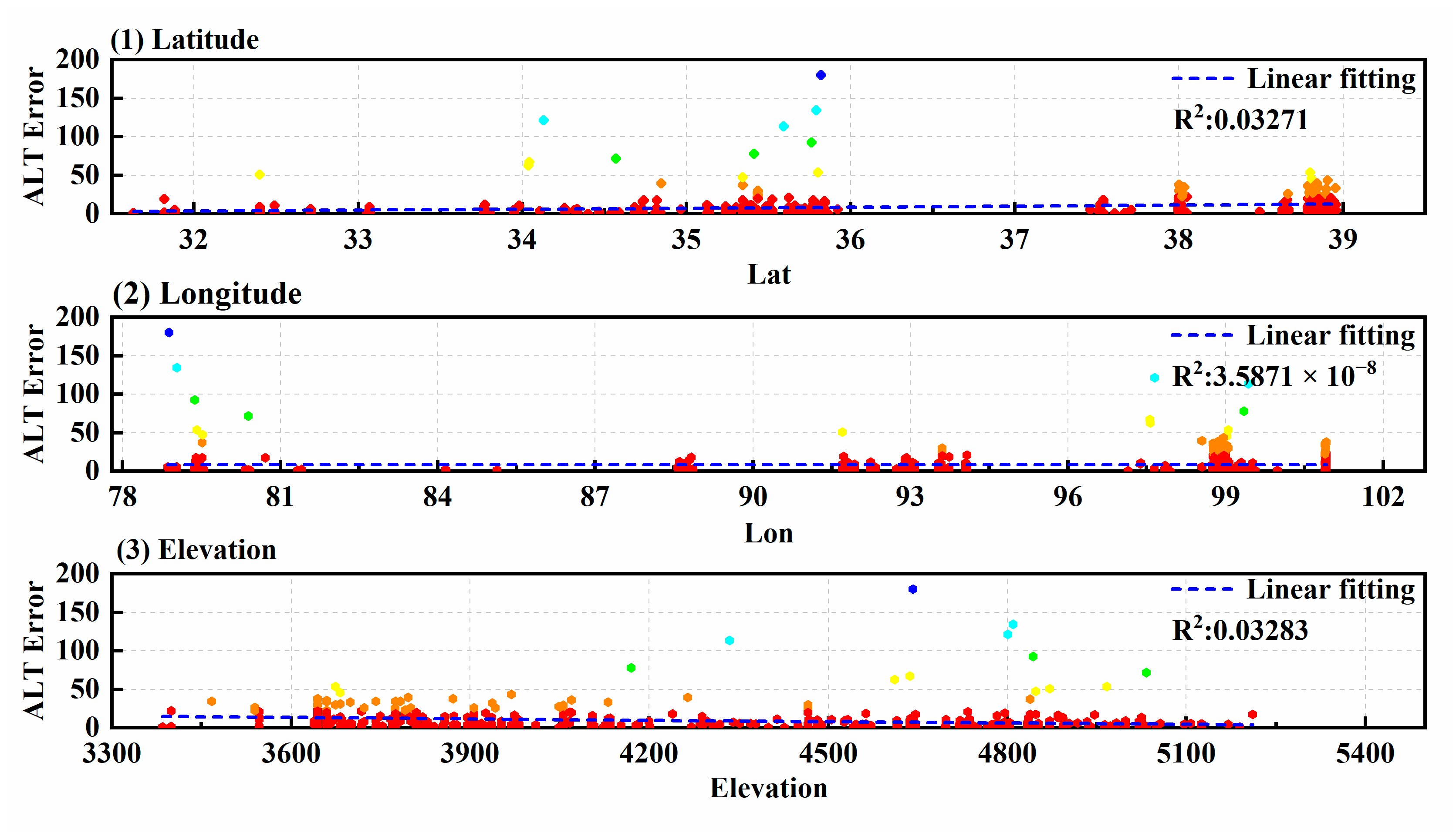
4.3. Analysis of ALT Influencing Factors
5. Discussion
6. Conclusions
Author Contributions
Funding
Data Availability Statement
Acknowledgments
Conflicts of Interest
Abbreviations
| ALT | Active Layer Thickness |
| QTP | Qinghai-Tibet Plateau |
| LST | Land Surface Temperature |
| DDF | Degree Days Freezing |
| DDT | Degree Days Thawing |
References
- Brown, R.J.E.; Kupsch, W.O. Permafrost terminology. Biul. Peryglac. 1992, 32, 1–176. [Google Scholar]
- French, H.M. The Periglacial Environment; John Wiley & Sons: Hoboken, NJ, USA, 2017. [Google Scholar]
- Guo, D.; Wang, H. CMIP5 permafrost degradation projection: A comparison among different regions. J. Geophys. Res. Atmos. 2016, 121, 4499–4517. [Google Scholar] [CrossRef]
- Heginbottom, J.A. Permafrost mapping: A review. Prog. Phys. Geogr. 2002, 26, 623–642. [Google Scholar] [CrossRef]
- Michaelides, R.J.; Schaefer, K.; Zebker, H.A.; Parsekian, A.; Liu, L.; Chen, J.; Natali, S.; Ludwig, S.; Schaefer, S.R. Inference of the impact of wildfire on permafrost and active layer thickness in a discontinuous permafrost region using the remotely sensed active layer thickness (ReSALT) algorithm. Environ. Res. Lett. 2019, 14, 035007. [Google Scholar] [CrossRef]
- Intergovernmental Panel on Climate Change. Climate change 2007: The physical science basis. Agenda 2007, 6, 333. [Google Scholar]
- Yan, D.; Feng, M.; Hu, Z.; Xu, J.; Li, X. Improving Permafrost Mapping in Southern Tibetan Plateau Using Machine Learning and Rock Glacier Inventory. Permafr. Periglac. Process. 2025, 36, 230–244. [Google Scholar] [CrossRef]
- Ran, Y.; Cheng, G.; Dong, Y.; Hjort, J.; Lovecraft, A.L.; Kang, S.; Tan, M.; Li, X. Permafrost degradation increases risk and large future costs of infrastructure on the Third Pole. Commun. Earth Environ. 2022, 3, 238. [Google Scholar] [CrossRef]
- Hjort, J.; Streletskiy, D.; Doré, G.; Wu, Q.; Bjella, K.; Luoto, M. Impacts of permafrost degradation on infrastructure. Nat. Rev. Earth Environ. 2022, 3, 24–38. [Google Scholar] [CrossRef]
- Wu, Q.; Zhang, T. Recent permafrost warming on the Qinghai-Tibetan Plateau. J. Geophys. Res. Atmos. 2008, 113, D13. [Google Scholar] [CrossRef]
- Zhao, L.; Wu, Q.; Marchenko, S.; Sharkhuu, N. Thermal state of permafrost and active layer in Central Asia during the international polar year. Permafr. Periglac. Process. 2010, 21, 198–207. [Google Scholar] [CrossRef]
- Schuur, E.A.; McGuire, A.D.; Schädel, C.; Grosse, G.; Harden, J.W.; Hayes, D.J.; Hugelius, G.; Koven, C.D.; Kuhry, P.; Lawrence, D.M. Climate change and the permafrost carbon feedback. Nature 2015, 520, 171–179. [Google Scholar] [CrossRef]
- Mu, C.; Li, L.; Wu, X.; Zhang, F.; Jia, L.; Zhao, Q.; Zhang, T. Greenhouse gas released from the deep permafrost in the northern Qinghai-Tibetan Plateau. Sci. Rep. 2018, 8, 4205. [Google Scholar] [CrossRef]
- Miner, K.R.; D’Andrilli, J.; Mackelprang, R.; Edwards, A.; Malaska, M.J.; Waldrop, M.P.; Miller, C.E. Emergent biogeochemical risks from Arctic permafrost degradation. Nat. Clim. Change 2021, 11, 809–819. [Google Scholar] [CrossRef]
- Hinkel, K.; Paetzold, F.; Nelson, F.; Bockheim, J. Patterns of soil temperature and moisture in the active layer and upper permafrost at Barrow, Alaska: 1993–1999. Glob. Planet. Change 2001, 29, 293–309. [Google Scholar] [CrossRef]
- Xiaodong, W.; Tonghua, W. Permafrost degradation has important effects on climate and human society. Chin. J. Nat. 2020, 42, 425–431. [Google Scholar]
- Brown, J.; Hinkel, K.M.; Nelson, F. The circumpolar active layer monitoring (CALM) program: Research designs and initial results. Polar Geogr. 2000, 24, 166–258. [Google Scholar] [CrossRef]
- Park, H.; Kim, Y.; Kimball, J.S. Widespread permafrost vulnerability and soil active layer increases over the high northern latitudes inferred from satellite remote sensing and process model assessments. Remote Sens. Environ. 2016, 175, 349–358. [Google Scholar] [CrossRef]
- Shen, T.; Jiang, P.; Ju, Q.; Yu, Z.; Chen, X.; Lin, H.; Zhang, Y. Changes in permafrost spatial distribution and active layer thickness from 1980 to 2020 on the Tibet Plateau. Sci. Total Environ. 2023, 859, 160381. [Google Scholar] [CrossRef]
- Li, G.; Zhang, M.; Pei, W.; Melnikov, A.; Khristoforov, I.; Li, R.; Yu, F. Changes in permafrost extent and active layer thickness in the Northern Hemisphere from 1969 to 2018. Sci. Total Environ. 2022, 804, 150182. [Google Scholar] [CrossRef]
- Anisimov, O.A.; Shiklomanov, N.I.; Nelson, F.E. Global warming and active-layer thickness: Results from transient general circulation models. Glob. Planet. Change 1997, 15, 61–77. [Google Scholar] [CrossRef]
- Stefan, J. Über die Theorie der Eisbildung, insbesondere über die Eisbildung im Polarmeere. Annalen der Physik 1891, 278, 269–286. [Google Scholar] [CrossRef]
- Wang, K.; Jafarov, E.; Overeem, I. Sensitivity evaluation of the Kudryavtsev permafrost model. Sci. Total Environ. 2020, 720, 137538. [Google Scholar] [CrossRef] [PubMed]
- Smith, S.L.; O’Neill, H.B.; Isaksen, K.; Noetzli, J.; Romanovsky, V.E. The changing thermal state of permafrost. Nat. Rev. Earth Environ. 2022, 3, 10–23. [Google Scholar] [CrossRef]
- Guo, D.; Wang, H. Simulated historical (1901–2010) changes in the permafrost extent and active layer thickness in the Northern Hemisphere. J. Geophys. Res. Atmos. 2017, 122, 12285–12295. [Google Scholar] [CrossRef]
- Chen, H.; Nan, Z.; Zhao, L.; Ding, Y.; Chen, J.; Pang, Q. Noah modelling of the permafrost distribution and characteristics in the West Kunlun area, Qinghai-Tibet Plateau, China. Permafr. Periglac. Process. 2015, 26, 160–174. [Google Scholar] [CrossRef]
- Aalto, J.; Karjalainen, O.; Hjort, J.; Luoto, M. Statistical forecasting of current and future circum-Arctic ground temperatures and active layer thickness. Geophys. Res. Lett. 2018, 45, 4889–4898. [Google Scholar] [CrossRef]
- Ni, J.; Wu, T.; Zhu, X.; Hu, G.; Zou, D.; Wu, X.; Li, R.; Xie, C.; Qiao, Y.; Pang, Q. Simulation of the present and future projection of permafrost on the Qinghai-Tibet Plateau with statistical and machine learning models. J. Geophys. Res. Atmos. 2021, 126, e2020JD033402. [Google Scholar] [CrossRef]
- Ran, Y.; Li, X.; Cheng, G.; Che, J.; Aalto, J.; Karjalainen, O.; Hjort, J.; Luoto, M.; Jin, H.; Obu, J. New high-resolution estimates of the permafrost thermal state and hydrothermal conditions over the Northern Hemisphere. Earth Syst. Sci. Data 2022, 14, 865–884. [Google Scholar] [CrossRef]
- Drucker, H.; Burges, C.J.; Kaufman, L.; Smola, A.; Vapnik, V. Support vector regression machines. Adv. Neural Inf. Process. Syst. 1996, 9, 155–161. [Google Scholar]
- Breiman, L. Random forests. Mach. Learn. 2001, 45, 5–32. [Google Scholar] [CrossRef]
- Chen, T.; Guestrin, C. Xgboost: A scalable tree boosting system. In Proceedings of the 22nd ACM Sigkdd International Conference on Knowledge Discovery and Data Mining, San Francisco, CA, USA, 13–17 August 2016; pp. 785–794. [Google Scholar]
- Mahanta, K.K.; Pradhan, I.P.; Gupta, S.K.; Shukla, D.P. Assessing Machine Learning and Statistical Methods for Rock Glacier-Based Permafrost Distribution in Northern Kargil Region. Permafr. Periglac. Process. 2024, 35, 262–277. [Google Scholar] [CrossRef]
- Liu, Q.; Niu, J.; Lu, P.; Dong, F.; Zhou, F.; Meng, X.; Xu, W.; Li, S.; Hu, B.X. Interannual and seasonal variations of permafrost thaw depth on the Qinghai-Tibetan plateau: A comparative study using long short-term memory, convolutional neural networks, and random forest. Sci. Total Environ. 2022, 838, 155886. [Google Scholar] [CrossRef] [PubMed]
- Bonnaventure, P.P.; Lamoureux, S.F. The active layer: A conceptual review of monitoring, modelling techniques and changes in a warming climate. Prog. Phys. Geogr. 2013, 37, 352–376. [Google Scholar] [CrossRef]
- Wei, Z.; Du, Z.; Wang, L.; Zhong, W.; Lin, J.; Xu, Q.; Xiao, C. Sedimentary organic carbon storage of thermokarst lakes and ponds across Tibetan permafrost region. Sci. Total Environ. 2022, 831, 154761. [Google Scholar] [CrossRef]
- Wei, R.; Hu, X.; Zhao, S. Changes in the Distribution of Thermokarst Lakes on the Qinghai-Tibet Plateau from 2015 to 2020. Remote Sens. 2025, 17, 1174. [Google Scholar] [CrossRef]
- Wang, S.; Niu, F.; Chen, J.; Dong, Y. Permafrost research in China related to express highway construction. Permafr. Periglac. Process. 2020, 31, 406–416. [Google Scholar] [CrossRef]
- Ran, Y.; Li, X.; Cheng, G.; Nan, Z.; Che, J.; Sheng, Y.; Wu, Q.; Jin, H.; Luo, D.; Tang, Z. Mapping the permafrost stability on the Tibetan Plateau for 2005–2015. Sci. China Earth Sci. 2021, 64, 62–79. [Google Scholar] [CrossRef]
- Yu, Q.; Zhang, Z.; Wang, G.; Guo, L.; Wang, X.; Wang, P.; Bao, Z. Analysis of tower foundation stability along the Qinghai–Tibet Power Transmission Line and impact of the route on the permafrost. Cold Reg. Sci. Technol. 2016, 121, 205–213. [Google Scholar] [CrossRef]
- Ran, Y.; Jorgenson, M.T.; Li, X.; Jin, H.; Wu, T.; Li, R.; Cheng, G. Biophysical permafrost map indicates ecosystem processes dominate permafrost stability in the Northern Hemisphere. Environ. Res. Lett. 2021, 16, 095010. [Google Scholar] [CrossRef]
- Abatzoglou, J.T.; Dobrowski, S.Z.; Parks, S.A.; Hegewisch, K.C. TerraClimate, a high-resolution global dataset of monthly climate and climatic water balance from 1958–2015. Sci. Data 2018, 5, 170191. [Google Scholar] [CrossRef]
- Niu, S.; Sun, M.; Wang, G.; Wang, W.; Yao, X.; Zhang, C. Glacier change and its influencing factors in the northern part of the Kunlun Mountains. Remote Sens. 2023, 15, 3986. [Google Scholar] [CrossRef]
- Wang, G.; Hao, X.; Yao, X.; Wang, J.; Li, H.; Chen, R.; Liu, Z. Simulations of snowmelt runoff in a high-altitude mountainous area based on big data and machine learning models: Taking the Xiying River basin as an example. Remote Sens. 2023, 15, 1118. [Google Scholar] [CrossRef]
- Poggio, L.; De Sousa, L.M.; Batjes, N.H.; Heuvelink, G.B.; Kempen, B.; Ribeiro, E.; Rossiter, D. SoilGrids 2.0: Producing soil information for the globe with quantified spatial uncertainty. Soil 2021, 7, 217–240. [Google Scholar] [CrossRef]
- Guangyue, L.; Lin, Z.; Changwei, X.; Qiangqiang, P.; Erji, D.; Yongping, Q. Variation characteristics and impact factors of the depth of zero annual amplitude of ground temperature in permafrost regions on the Tibetan Plateau. J. Glaciol. Geocryol. 2016, 38, 1189–1200. [Google Scholar]
- Wu, Q.; Dong, X.; Liu, Y.; Jin, H. Responses of permafrost on the Qinghai-Tibet Plateau, China, to climate change and engineering construction. Arct. Antarct. Alp. Res. 2007, 39, 682–687. [Google Scholar] [CrossRef]
- Li, R.; Zhao, L.; Ding, Y.; Wu, T.; Xiao, Y.; Du, E.; Liu, G.; Qiao, Y. Temporal and spatial variations of the active layer along the Qinghai-Tibet Highway in a permafrost region. Chin. Sci. Bull. 2012, 57, 4609–4616. [Google Scholar] [CrossRef]
- Wang, Q.; Jin, H.; Zhang, T.; Cao, B.; Peng, X.; Wang, K.; Xiao, X.; Guo, H.; Mu, C.; Li, L. Hydro-thermal processes and thermal offsets of peat soils in the active layer in an alpine permafrost region, NE Qinghai-Tibet plateau. Glob. Planet. Change 2017, 156, 1–12. [Google Scholar] [CrossRef]
- Zou, D.; Zhao, L.; Sheng, Y.; Chen, J.; Hu, G.; Wu, T.; Wu, J.; Xie, C.; Wu, X.; Pang, Q. A new map of permafrost distribution on the Tibetan Plateau. Cryosphere 2017, 11, 2527–2542. [Google Scholar] [CrossRef]
- Wu, Q.; Zhang, T. Changes in active layer thickness over the Qinghai-Tibetan Plateau from 1995 to 2007. J. Geophys. Res. Atmos. 2010, 115, D09107. [Google Scholar] [CrossRef]
- Cao, B.; Zhang, T.; Peng, X.; Mu, C.; Wang, Q.; Zheng, L.; Wang, K.; Zhong, X. Thermal characteristics and recent changes of permafrost in the upper reaches of the Heihe River Basin, Western China. J. Geophys. Res. Atmos. 2018, 123, 7935–7949. [Google Scholar] [CrossRef]
- Wang, C.; Zhao, L.; Ma, L.; Hu, G.; Zhang, L.; Zou, D.; Xing, Z.; Xiao, Y.; Zhou, H.; Qiao, Y. Precipitation adjustment by the OTT Parsivel2 in the central Qinghai–Tibet Plateau. Earth Surf. Process. Landf. 2024, 49, 2424–2441. [Google Scholar] [CrossRef]
- Geurts, P.; Ernst, D.; Wehenkel, L. Extremely randomized trees. Mach. Learn. 2006, 63, 3–42. [Google Scholar] [CrossRef]
- Galelli, S.; Castelletti, A. Assessing the predictive capability of randomized tree-based ensembles in streamflow modelling. Hydrol. Earth Syst. Sci. 2013, 17, 2669–2684. [Google Scholar] [CrossRef]
- Prokhorenkova, L.; Gusev, G.; Vorobev, A.; Dorogush, A.V.; Gulin, A. CatBoost: Unbiased boosting with categorical features. Adv. Neural Inf. Process. Syst. 2018, 31, 1–11. [Google Scholar]
- Hancock, J.T.; Khoshgoftaar, T.M. CatBoost for big data: An interdisciplinary review. J. Big Data 2020, 7, 94. [Google Scholar] [CrossRef]
- Dietterich, T.G. Ensemble methods in machine learning. In Proceedings of the International Workshop on Multiple Classifier Systems, Cagliari, Italy, 21–23 June 2000; pp. 1–15. [Google Scholar]
- Zhou, Z.-H. Ensemble Methods: Foundations and Algorithms; CRC Press: Boca Raton, FL, USA, 2025. [Google Scholar]
- Sill, J.; Takács, G.; Mackey, L.; Lin, D. Feature-weighted linear stacking. arXiv 2009, arXiv:0911.0460. [Google Scholar]
- Peng, X.; Zhang, T.; Cao, B.; Wang, Q.; Wang, K.; Shao, W.; Guo, H. Changes in freezing-thawing index and soil freeze depth over the Heihe River Basin, western China. Arct. Antarct. Alp. Res. 2016, 48, 161–176. [Google Scholar] [CrossRef]
- Biskaborn, B.K.; Smith, S.L.; Noetzli, J.; Matthes, H.; Vieira, G.; Streletskiy, D.A.; Schoeneich, P.; Romanovsky, V.E.; Lewkowicz, A.G.; Abramov, A. Permafrost is warming at a global scale. Nat. Commun. 2019, 10, 264. [Google Scholar] [CrossRef]
- Yi, Y.; Kimball, J.S.; Rawlins, M.A.; Moghaddam, M.; Euskirchen, E.S. The role of snow cover affecting boreal-arctic soil freeze–thaw and carbon dynamics. Biogeosciences 2015, 12, 5811–5829. [Google Scholar] [CrossRef]
- Morse, P.; Wolfe, S.; Kokelj, S.; Gaanderse, A. The occurrence and thermal disequilibrium state of permafrost in forest ecotopes of the Great Slave Region, Northwest Territories, Canada. Permafr. Periglac. Process. 2016, 27, 145–162. [Google Scholar] [CrossRef]
- Fisher, J.P.; Estop-Aragonés, C.; Thierry, A.; Charman, D.J.; Wolfe, S.A.; Hartley, I.P.; Murton, J.B.; Williams, M.; Phoenix, G.K. The influence of vegetation and soil characteristics on active-layer thickness of permafrost soils in boreal forest. Glob. Change Biol. 2016, 22, 3127–3140. [Google Scholar] [CrossRef] [PubMed]
- Fu, Q.; Hou, R.; Li, T.; Wang, M.; Yan, J. The functions of soil water and heat transfer to the environment and associated response mechanisms under different snow cover conditions. Geoderma 2018, 325, 9–17. [Google Scholar] [CrossRef]
- Andersland, O.B.; Ladanyi, B. Frozen Ground Engineering; John Wiley & Sons: Hoboken, NJ, USA, 2003. [Google Scholar]
- Zhang, T. Influence of the seasonal snow cover on the ground thermal regime: An overview. Rev. Geophys. 2005, 43, 4. [Google Scholar] [CrossRef]
- Jorgenson, M.T.; Romanovsky, V.; Harden, J.; Shur, Y.; O’Donnell, J.; Schuur, E.A.; Kanevskiy, M.; Marchenko, S. Resilience and vulnerability of permafrost to climate change. Can. J. For. Res. 2010, 40, 1219–1236. [Google Scholar] [CrossRef]
- Wu, B.; Zhang, M.; Zeng, H.; Tian, F.; Potgieter, A.B.; Qin, X.; Yan, N.; Chang, S.; Zhao, Y.; Dong, Q. Challenges and opportunities in remote sensing-based crop monitoring: A review. Natl. Sci. Rev. 2023, 10, nwac290. [Google Scholar] [CrossRef]
- Song, C.; Huang, B.; Ke, L.; Richards, K.S. Remote sensing of alpine lake water environment changes on the Tibetan Plateau and surroundings: A review. ISPRS J. Photogramm. Remote Sens. 2014, 92, 26–37. [Google Scholar] [CrossRef]
- Ferguglia, O.; Palazzi, E.; Arnone, E. Elevation dependent change in ERA5 precipitation and its extremes. Clim. Dyn. 2024, 62, 8137–8153. [Google Scholar] [CrossRef]
- Li, W.; Zhao, L.; Wu, X.; Wang, S.; Sheng, Y.; Ping, C.; Zhao, Y.; Fang, H.; Shi, W. Soil distribution modeling using inductive learning in the eastern part of permafrost regions in Qinghai–Xizang (Tibetan) Plateau. Catena 2015, 126, 98–104. [Google Scholar] [CrossRef]
- Wang, Z.; Kim, Y.; Seo, H.; Um, M.-J.; Mao, J. Permafrost response to vegetation greenness variation in the Arctic tundra through positive feedback in surface air temperature and snow cover. Environ. Res. Lett. 2019, 14, 044024. [Google Scholar] [CrossRef]
- Zhang, X.; Zhang, H.; Wang, C.; Tang, Y.; Zhang, B.; Wu, F.; Wang, J.; Zhang, Z. Active layer thickness retrieval over the Qinghai-Tibet Plateau using Sentinel-1 multitemporal InSAR monitored Permafrost subsidence and temporal-spatial multilayer soil moisture data. IEEE Access 2020, 8, 84336–84351. [Google Scholar] [CrossRef]
- Jia, S.; Zhang, T.; Hao, J.; Li, C.; Michaelides, R.; Shao, W.; Wei, S.; Wang, K.; Fan, C. Spatial Variability of Active Layer Thickness along the Qinghai–Tibet Engineering Corridor Resolved Using Ground-Penetrating Radar. Remote Sens. 2022, 14, 5606. [Google Scholar] [CrossRef]
- Zhao, L.; Zou, D.; Hu, G.; Du, E.; Pang, Q.; Xiao, Y.; Li, R.; Sheng, Y.; Wu, X.; Sun, Z. Changing climate and the permafrost environment on the Qinghai–Tibet (Xizang) plateau. Permafr. Periglac. Process. 2020, 31, 396–405. [Google Scholar] [CrossRef]
- Yang, Y.; You, Q.; Zuo, Z.; Zhang, Y.; Liu, Z.; Kang, S.; Zhai, P. Elevation dependency of temperature trend over the Qinghai-Tibetan Plateau during 1901–2015. Atmos. Res. 2023, 290, 106791. [Google Scholar] [CrossRef]


| Machine Learning Model Name | RMSE (cm) | MAE (cm) | R2 | MAPE |
|---|---|---|---|---|
| CatBoost | 37.838 | 25.552 | 0.825 | 0.131 |
| Random Forest | 39.036 | 26.263 | 0.816 | 0.137 |
| Extra Trees | 39.293 | 25.272 | 0.811 | 0.130 |
| Light Gradient Boosting Machine | 40.643 | 27.017 | 0.801 | 0.137 |
| Gradient Boosting | 41.514 | 28.105 | 0.789 | 0.144 |
| Extreme Gradient Boosting | 42.302 | 27.678 | 0.782 | 0.139 |
| Model | RMSE (cm) | MAE (cm) | R2 | MAPE |
|---|---|---|---|---|
| SCE model | 32.680 | 20.713 | 0.873 | 0.104 |
| Linner | 69.876 | 53.767 | 0.429 | 0.273 |
| Δ-error | 37.196 | 33.054 | 0.444 | 0.169 |
| References | Study Area | Model Name | RMSE (cm) | R2 |
|---|---|---|---|---|
| This research | QTP | SCE-ALT | 32.68 | 0.873 |
| [19] | QTP | XGB-R | 55.4 | 0.558 |
| Stefan | 56.3 | 0.543 | ||
| [28] | QTP | GLM-ALT | 78 | 0.33 |
| GAM-ALT | 77 | 0.35 | ||
| GBM-ALT | 74 | 0.40 | ||
| RF-ALT | 69 | 0.51 | ||
| Ensemble-ALT | 71 | 0.46 | ||
| [75] | Tuotuohe to Wudaoliang (90.715 93.751N, 34.204 35.836E) | Point Scale Soil Moisture Data and Seasonal Subsidence | 92 | 0.63 |
| SMAP L4 Soil Moisture Data and Seasonal Subsidence | 70 | 0.67 | ||
| [76] | Extends from Xidatan to Ando (32.53–35.62N, 91.6–94.06E) | Statistical Estimation Model | 39 | 0.52 |
Disclaimer/Publisher’s Note: The statements, opinions and data contained in all publications are solely those of the individual author(s) and contributor(s) and not of MDPI and/or the editor(s). MDPI and/or the editor(s) disclaim responsibility for any injury to people or property resulting from any ideas, methods, instructions or products referred to in the content. |
© 2025 by the authors. Licensee MDPI, Basel, Switzerland. This article is an open access article distributed under the terms and conditions of the Creative Commons Attribution (CC BY) license (https://creativecommons.org/licenses/by/4.0/).
Share and Cite
Wang, G.; Niu, S.; Yan, D.; Liang, S.; Su, Y.; Wang, W.; Yin, T.; Sun, X.; Wan, L. Simulation of Active Layer Thickness Based on Multi-Source Remote Sensing Data and Integrated Machine Learning Models: A Case Study of the Qinghai-Tibet Plateau. Remote Sens. 2025, 17, 2006. https://doi.org/10.3390/rs17122006
Wang G, Niu S, Yan D, Liang S, Su Y, Wang W, Yin T, Sun X, Wan L. Simulation of Active Layer Thickness Based on Multi-Source Remote Sensing Data and Integrated Machine Learning Models: A Case Study of the Qinghai-Tibet Plateau. Remote Sensing. 2025; 17(12):2006. https://doi.org/10.3390/rs17122006
Chicago/Turabian StyleWang, Guoyu, Shuting Niu, Dezhao Yan, Sihai Liang, Yanan Su, Wei Wang, Tao Yin, Xingliang Sun, and Li Wan. 2025. "Simulation of Active Layer Thickness Based on Multi-Source Remote Sensing Data and Integrated Machine Learning Models: A Case Study of the Qinghai-Tibet Plateau" Remote Sensing 17, no. 12: 2006. https://doi.org/10.3390/rs17122006
APA StyleWang, G., Niu, S., Yan, D., Liang, S., Su, Y., Wang, W., Yin, T., Sun, X., & Wan, L. (2025). Simulation of Active Layer Thickness Based on Multi-Source Remote Sensing Data and Integrated Machine Learning Models: A Case Study of the Qinghai-Tibet Plateau. Remote Sensing, 17(12), 2006. https://doi.org/10.3390/rs17122006