Abstract
Moso bamboo forests, recognized as a distinctive and significant forest resource in subtropical China, contribute substantially to efficient carbon sequestration. The accurate assessment of the aboveground biomass (AGB) in Moso bamboo forests is crucial for evaluating their impact on the carbon balance within forest ecosystems at a regional scale. In this study, we focused on the Moso bamboo forest located in Shanchuan Township, Zhejiang Province, China. The primary objective was to utilize various data sources, namely UAV-LiDAR (UL), Sentinel-2 (ST), and a combination of UAV-LiDAR with Sentinel-2 (UL + ST). Employing the Boruta algorithm, we carefully selected characterization variables for analysis. Our investigation delved into establishing correlations between UAV-LiDAR characterization parameters, Sentinel-2 feature parameters, and the aboveground biomass (AGB) of the Moso bamboo forest. Ground survey data on Moso bamboo forest biomass served as the basis for our analysis. To enhance the accuracy of AGB estimation in the Moso bamboo forest, we employed three distinct modeling techniques: multivariate linear regression (MLR), support vector regression (SVR), and random forest (RF). Through this approach, we aimed to compare the impact of different data sources and modeling methods on the precision of AGB estimation in the studied bamboo forest. This study revealed that (1) the point cloud intensity of UL, the variables of canopy cover (CC), gap fraction (GF), and leaf area index (LAI) reflect the structure of Moso bamboo forests, and the variables indicating the height of the forest stand (AIH1, AIHiq, and Hiq) had a significant effect on the AGB of Moso bamboo forests, significantly impact Moso bamboo forest AGB. Vegetation indices such as DVI and SAVI in ST also exert a considerable effect on Moso bamboo forest AGB. (2) AGB estimation models constructed based on UL consistently demonstrated higher accuracy compared with ST, achieving R2 values exceeding 0.7. Regardless of the model used, UL consistently delivered superior accuracy in Moso bamboo forest AGB estimation, with RF achieving the highest precision at R2 = 0.88. (3) Integration of ST with UL substantially improved the accuracy of AGB estimation for Moso bamboo forests across all three models. Specifically, using RF, the accuracy of AGB estimation increased by 97.7%, with R2 reaching 0.89 and RMSE reduced by 124.4%. As a result, the incorporation of LiDAR data, which reflects the stand structure, has proven to enhance the accuracy of aboveground biomass (AGB) estimation in Moso bamboo forests when combined with multispectral remote sensing data. This integration serves as an effective solution to address the limitations of single optical remote sensing methods, which often suffer from signal saturation, leading to lower accuracy in estimating Moso bamboo forest biomass. This approach offers a novel perspective and opens up new possibilities for improving the precision of Moso bamboo forest biomass estimation through the utilization of multiple remote sensing sources.
1. Introduction
Forest ecosystems play a crucial role in terrestrial ecosystems, serving as highly productive communities that store approximately 80% of carbon above the ground and around 20% below the ground [1]. Forests have a crucial function in the global carbon cycle, as their above-ground biomass (AGB) acts as a pivotal factor for assessing the carbon equilibrium within these ecosystems. Precise determination of AGB in forests holds great importance in evaluating their capacity as carbon sinks [2].
Bamboo is an evergreen perennial flowering plant in the subfamily Bamboo of the family Gramineae, which is mainly distributed in tropical and subtropical regions, among which the most widely distributed bamboo species is the Moso bamboo (Phyllostachys edulis) [3]. Moso bamboo forests are characterized by fast growth and short harvesting cycles, and their distribution area has increased in the past 20 years. In the context of global climate change, the significant carbon sequestration and emission reduction in Moso bamboo forests have been given more attention and importance. The above-ground biomass of bamboo forests is an important research basis for carbon cycling in bamboo forest ecosystems [4,5].
Traditional forest AGB estimates are mainly obtained through field surveys combined with anisotropic growth modeling or destructive sampling [6,7,8], which, although capable of obtaining forest AGB extremely accurately, often requires a great deal of time and effort [9]. Remote sensing earth observation technology has the characteristics of real-time, dynamic, large-area synchronous monitoring and information-rich, which greatly improves the efficiency of working traditional methods of AGB estimation and has become one of the important means of estimating forest AGB [10,11,12,13,14,15,16,17,18].
Most of the current research on remote sensing estimation of aboveground biomass of Moso bamboo forest only uses passive satellite remote sensing data [16,19,20,21]. Most are based on a single time-phase remote sensing vegetation indices, spectral information of the texture, and other features. The canopies of Moso bamboo forests are connected with each other into a horizontal depressed state, and the forest stand structure is similar, which makes biomass estimation in Moso bamboo forests difficult. Previous studies have also proved the accuracy of estimation of the AGB of Moso bamboo forests using optical sensors to have low accuracy [22]. For example, Du et al. [23] explored the relationship between Landsat TM imagery and Moso bamboo forest AGB and proved that the highest correlation coefficient between Moso bamboo forest AGB and TM-driven vegetation index was 0.48. At the same site, Du et al. [24] constructed a partial least squares-based model for estimating Moso bamboo forest AGB based on Landsat TM satellite remote sensing data, with an R2 of 0.55. Chen et al. [25] used sentinel-2 data to identify key variables related to bamboo forest AGB using a random forest algorithm.
Numerous researchers have come to the realization that passive optical remote sensing encounters a significant issue with signal saturation, potentially affecting the precision of forest AGB estimation [26]. Being an active remote sensing technology [16], Light Detection And Ranging (LiDAR) emits laser pulses that can effectively penetrate the canopy, generating extremely rich 3D point cloud data of forests, which can achieve an accurate estimation of forest tree height and canopy structure, thus attracting a large number of scholars to carry out forest AGB research using LiDAR. This has attracted a large number of scholars to use LiDAR to carry out forest AGB research [27], such as Mariano et al. [28], who explored the AGB estimation model construction method based on LiDAR height, intensity, or a combination of height and intensity data. Zhang et al. [29] also accurately and successfully estimated the AGB of the urban forest based on the UAV-LiDAR and coupled it with the structural characteristics of the canopy.
LiDAR can directly measure the vertical structure and horizontal characteristics of the forest canopy, which provides a good basis for the high correlation between the biomass of the Moso bamboo forest and the LiDAR metrics. Compared with previous studies, the results of Cao et al. [30] in estimating the AGB of Moso bamboo forests using Airborne LiDAR (R2 = 0.59~0.87) have improved remarkably, which proves the potential advantages of LiDAR for estimating the biomass of Moso bamboo forests.
The rich spectral characteristics of passive remote sensing enable the retrieval of chlorophyll, which is closely associated with vegetation biomass growth. Additionally, vegetation indices derived from this data source can be utilized to characterize aboveground biomass (AGB). On the other hand, LiDAR technology offers valuable insights into the vertical composition of forests, including heights, which serve as crucial indicators for AGB estimation. Therefore, finding effective approaches to integrate the strengths of LiDAR and passive optical remote sensing data has been a prominent concern among both domestic and international researchers aiming for more precise forest AGB estimation [31]. For example, Laurin et al. [32] fused LiDAR data and hyperspectral data to estimate tropical forest AGB, and the results showed that the synergistic use of active and passive remote sensing data estimation could improve the estimation accuracy of the forest AGB; the results of Rana et al. [33] also showed that the forest AGB estimation results were significantly improved after the UAV-LiDAR data combined with the optical remote sensing data. Wang et al. [34] constructed a point-line-polygon framework for regional coniferous forest AGB mapping using field survey data, UAV-LiDAR strip data, and Sentinel-1 and Sentinel-2 imagery and analyzed the potential of multiscale wavelet transform texture and tree species stratification on the accuracy of coniferous forest AGB estimation in North China, and the highest accuracy of AGB estimation was found for creosote bush, with an R2 of 0.78; Jiang et al. [35] used Sentinel-2 images provided by GEE as a medium for continuous AGB mapping with ICESat-2, and the results showed that the estimation error of each model was significantly reduced by adding the LiDAR variable of ICESat-2 to the AGB compared with using Sentinel-2 alone. Therefore, the combination of optical remote sensing data, which characterizes the spectral features of forests, and LiDAR data, which reflects the structure of forest stands, is a new way to estimate the AGB of Moso bamboo forests.
Models are the bridge between ground-truthed AGB linked remote sensing data to achieve large-scale forest AGB spatiotemporal estimation, so the general practice of forest AGB remote sensing estimation is achieved by establishing regression relationships between ground-truthed data and feature variables extracted from remote sensing data [36]. Therefore, the screening of feature variables and model selection of remote sensing data becomes the key to ensuring the accuracy of AGB estimation [37,38]. Boruta is a commonly used feature screening algorithm, which is capable of automatically identifying and selecting important features [39]. Boruta selects variables with a high impact on prediction accuracy by providing “variable importance” [40]. In recent years, the Boruta algorithm has been used by many scholars for feature variable selection and biomass estimation due to its robustness and stability [41,42,43]. For example, Swati et al. [44] utilized the correlation of spectral and texture variables in a ground survey and Landsat 8 OLI data and used the Boruta feature selection method to reduce 198 independent variables, such as wave bands, vegetation indices and texture features, to the correlation with ASTA and ASTA, and then reduced them to the correlation with ASTA. Independent variables were reduced to 29 variables related to AGB with an R2 of 0.83; Huang et al. [45] estimated the AGB of four forest types in Yunnan Province based on the variables extracted from environmental factors and the Boruta algorithm and utilized Landsat 8 OLI and Sentinel 2A composite imagery based on a machine learning algorithm.
The traditional multivariate linear regression (MLR) model is one of the most commonly used models for AGB estimation, but in reality, the relationship between AGB and remote sensing data is often non-linear, and it is difficult to meet the basic assumption that remote sensing variables are independent of each other, and therefore, the model error is large [23]. In recent years, RandomForest (RF) has been widely used in forest AGB estimation research because of its fast response speed, high prediction accuracy, and good robustness to outliers and noise points. Support vector regression (SVR) has also become an important method for estimating forest AGB using remotely sensed data by utilizing its use of small training sample data to produce higher estimation accuracy relative to other methods and by being able to solve both linear and non-linear problems [31,46,47]. For example, Tamiminia et al. [48] achieved the estimation of forest AGB in New York State and analyzed the inter-annual changes of AGB from 2001 to 2019 on the GEE cloud platform based on the random forest model using Landsat imagery, airborne LiDAR data, and ground data, and Yu et al. [49] analyzed the inter-annual changes of AGB from 2001 to 2019 for GF-2, Sentinel-2, and Landsat-8 Sentinel-2, and Landsat-8 remote sensing data, extracted vegetation indices, spectral indices and texture features for AGB prediction, established an AGB estimation model, and compared the estimation accuracies, and the results showed that the random forest model has a better estimation accuracy under the three types of different spatial resolutions of remote sensing data, which proves the feasibility of the random forest model for estimating AGB. Zhang et al. [50] studied the relationship between airborne LIDAR and the SAR year-month time series and multispectral data to synergistically estimate AGB using four prediction models, namely, RF, SVR, KNN, and MLPNN, and the results of the study showed that RF exhibited the best performance compared with other algorithms. Dong et al. [51] estimated the aboveground biomass of Lei Zhi forest using Worldview-2 and compared the performance of the convolutional neural network (CNN), randomized Forest (RF), artificial neural network (ANN), and support vector regression (SVR) algorithms in terms of band and vegetation index, and it was found that the accuracy of RF and SVR was slightly better than that of CNN.
This study took Moso bamboo forest in Shanchuan Township, Anji County as the research object, and based on the ground survey of Moso bamboo forest, three data sources, namely, single UAV-LiDAR data, single Sentinel-2 data, and UAV-LiDAR combined with Sentinel-2 data, were used to screen the feature parameters related to AGB of Moso bamboo forest based on Boruta algorithm, and to explore the correlation between the feature parameters of Sentinel-2 and the feature parameters of UAV-LiDAR and the AGB of Moso bamboo forest. 2 and UAV-LiDAR with Sentinel-2, to explore the correlation between Sentinel-2 and UAV-LiDAR feature parameters and Moso bamboo forest AGB; on the basis of the screening of variables, the remote sensing estimation model of aboveground biomass of Moso bamboo forest was constructed based on the three models of MLR, SVR, and RF, and the accuracy was verified using the ground data, so that the impacts of different data sources and modeling methods on the accuracy of AGB estimation of Moso bamboo forest were compared, and a new idea and method was developed for the quantitative estimation of Moso bamboo forest biomass. A new idea and method for quantitative estimation of bamboo forest biomass is provided.
2. The Study Area and Data Acquisition
2.1. The Study Area
The location of this study, depicted in Figure 1, is situated within the geographical coordinates of Shanchuan Township, Anji County, Huzhou City, Zhejiang Province in China, between longitude 119°37′28″~119°41′56″E and latitude 30°23′41″~30°29′13″N. The elevation of the study area varies between 500 and 1000 m and is characterized by a subtropical monsoon climate that offers ample sunshine, rainfall, and distinct seasons. This climatic condition provides an ideal environment for the flourishing growth of bamboo forests. Consequently, this region has earned its reputation as the ‘Bamboo Capital of China’ because of its tropical monsoon climate featuring abundant light, rainfall, and well-defined seasons conducive to thriving bamboo forests. The study area consisted entirely of pristine Moso bamboo forests, characterized by an average DBH of 10.9 cm and a canopy height ranging from 12 to 18 m. Additionally, there was a limited presence of understory shrubs and herbaceous plants.
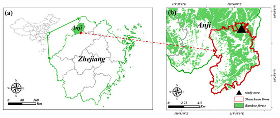
Figure 1.
Study area: (a) Anji County’s geographical position; (b) Geographical location of the specified research region.
2.2. The Process of Researching and Pre-processing Data
2.2.1. UAV-LiDAR Data Acquisition and Processing
As shown in Figure 2, on 17 April 2023, this study adopted H300-RT, an integrated digital acquisition system for airborne point cloud images, to acquire point cloud data in the study area. The flight height of the UAV is 80 m, the route spacing is 25 m, the side-overlap rate of data sampling is 50%, the laser wavelength is 905 nm, and the laser emission frequency is 300 kHz. The sensor records the first echo information of the laser pulse, the maximum scanning angle is ±15°, the scanning frequency is 20 Hz, the scanning speed is 640,000 points/s, and the average point cloud density is 400 pts/m2. Other attributes of the LiDAR scanner and UAV flight parameters are shown in Table 1.
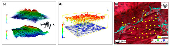
Figure 2.
Acquisition and pre-processing of data through remote sensing techniques: (a) resolved UAV-LiDAR raw point cloud; (b) normalized point cloud image of sample plots; (c) A captured image of the study area using Sentinel-2 and the layout of sample plots.

Table 1.
Characteristics of UAV-LiDAR sensor and flight parameters in this study.
Data obtained using UAV-LIDAR are obtained by coordinate solution, GNSS difference, trajectory solution, and data fusion to obtain the original LIDAR point cloud. The height threshold method is used to denoise the denoised point cloud data. The improved progressive TIN densification (IPTD) is used to separate ground points and non-ground points [52,53]. The inverse distance weighted (IDW) method is used to calculate the average height of laser points within pixels to obtain the digital elevation model (DEM) with a spatial resolution of 0.3 m. Finally, the DEM is used to normalize point cloud data to obtain normalized point cloud data for extracting forest parameters in the sample plot.
2.2.2. Sentinel-2 Data Acquisition and Processing
We opted for a Sentinel-2 remote sensing image taken on 8 April 2023 to align with the UAV-LiDAR data acquisition timing in our research. The selected image exhibited minimal cloud coverage, accounting for merely 1.67% within the designated research area. It encompassed a total of 12 spectral bands, including those that capture visible light, near-infrared, and short-wave infrared regions (refer to Figure 2c. For this research study, we accessed the chosen images from Sentinel-2 via the Google Earth Engine (GEE) platform utilizing the COPERNICUS/S2_SR_HARMONIZED dataset. Following that, we extracted area-wide images after implementing a de-clouding process based on the QA60 band for assessing image remote sensing quality. Moreover, to address variations in spatial resolution within spectral data of Sentinel-2, we performed resampling to achieve a consistent resolution of 10 m × 10 m.
2.2.3. Ground Survey Data and AGB Calculations
In this study area, a combined count of 35 sample plots measuring 30 m × 30 m was established for the Moso bamboo forest. The ground aboveground biomass (AGB) survey was conducted simultaneously with the acquisition of UAV-LiDAR data. To accurately determine the plot boundaries, real-time kinematics (RTK) technology was employed, ensuring a horizontal positioning error within ±2 cm and an elevation positioning error within ±5 cm, as depicted in Figure 3a,b. The survey incorporated the latitude, longitude, elevation, and incline of the selected location and the diameter at breast height in addition to the age of the Moso bamboo, as shown in Figure 3c. The estimation of aboveground biomass for individual Moso bamboo at the designated location was conducted utilizing Equation (1), and the model was established based on the Moso bamboo survey data in Zhejiang Province. At the 0.05 confidence level, the model’s prediction accuracy was 96.43%, and the total systematic error was −0.021%, so the model has a better estimation accuracy and a certain degree of adaptability [54].
where: The aboveground biomass (dry mass, kg) is represented by M and is determined based on the diameter at breast height (cm), denoted as D, and age indicated by A. The total aboveground biomass (AGB) of the sample plot was determined by summing up the AGB of each individual tree.
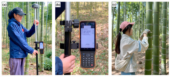
Figure 3.
Ground survey: (a,b) RTK positioning of sample plots (c) single-tree diameter at breast height measurement.
3. Research Methodology
3.1. UAV-LiDAR Data Feature Variable Settings
LiDAR data used in this study consist of a comprehensive set of 101 feature variables categorized into four groups: stand canopy structure features, stand height features, LiDAR point cloud density features, and LiDAR intensity. These details are presented in Table 2.
Table 2.
Feature variables extracted by UAV-LiDAR.
3.2. Sentinel-2 Remote Sensing Feature Variable Settings
These details can be found in Table 3. Among them, the spectral band represents the grayscale value of the original Sentinel-2 image band. Vegetation indices encompass various measures such as difference vegetation index (DVI), enhanced vegetation index (EVI), triangular vegetation index (TVI), ratio vegetation index (RVI), vegetation decay index (PSRI), normalized difference infrared index (NDII), normalized difference water content index (NDWI), normalized vegetation index (NDVI), normalized difference water index (MNDWI), soil adjusted vegetation Index (SAVI), normalized building index (NDBI), and chlorophyll index (Cire). Texture features were derived using a method based on a grey scale covariance matrix for four spectral bands: blue, green, red, and near-infrared. These included variance (VAR), homogeneity (HOM), contrast (CON), dissimilarity (DIS), entropy (ENT), angular binary index (ABI), normalized building index (NDBI), and chlorophyll index (Cire). Furthermore, we computed additional texture features such as angular second moment(ASM), correlation (COR), and cluster shade (SHA). To mitigate potential bias caused by different texture windows in texture information extraction [9], we calculated five GLCM textures with window sizes of 3 × 3, 5 × 5, 7 × 7, 9 × 9, and 11 × 11, resulting in a total of 160 texture eigenvalues. In this study, the combination of these texture variables, along with the original band grayscale values and vegetation indices, resulted in a comprehensive set of 184 Sentinel-2 remote sensing feature variables.
Table 3.
Feature variables extracted by Sentinel-2.
3.3. Feature Variable Screening Based on Boruta’s Algorithm
Boruta’s algorithm [39] is a random forest-based classification wrapper algorithm that efficiently identifies all features with high correlation to the outcome variable. Boruta’s feature selection algorithm builds multiple random forests by constructing shadow features that randomly order the original features, combining the original feature set, and iterating repeatedly to eliminate the original feature variables that are significantly less important than the shadow features, thus filtering out all features that are relevant to the dependent variable [78], and the score Z is the basis for filtering the important features. Z is obtained by dividing the mean accuracy loss by its standard deviation. The determination of the significance of the original feature depends on comparing its Z-score with the maximum Z-score (MZSA) in the shadow feature. Moreover, when Z < MZSA, the feature is rejected, while when Z > MZSA, the feature is accepted by the feature and is further statistically analyzed using a two-sided test to decide whether the special is selected [79]. In this research study, LiDAR data in Table 2 and the features of the Sentinel-2 image in Table 3 were screened using the bestglm package available in R.
3.4. Model Construction Methodology
3.4.1. Multiple Linear Regression Models
The multiple linear regression (MLR) technique is widely employed to estimate forest structural parameters using remotely sensed data. It enables the establishment of a linear relationship between one dependent variable and two or more independent variables, facilitating parameter estimation. The general expression for MLR is as follows:
where: remains a constant throughout the equation; the regression coefficients … indicate the extent to which each variable contributes to the dependent variable; , are variables that are not dependent on each other, and they correspond to the characterization variables listed in Table 3. In this study, the dependent variable Y represents the structural parameter of the estimated structure. In this research study, a comprehensive analysis was conducted by considering all potential combinations of variables through the utilization of full subset regression [80]. Subsequently, the most optimal combination of variables was chosen to construct a multiple linear regression (MLR) model with the aim of accurately estimating aboveground biomass (AGB) in bamboo forests at the sample level.
3.4.2. Support Vector Regression Model
The SVR model is a technique that employs support vector machines for analyzing regression problems. It utilizes classification methods to tackle the issue of limited sample size in regression analysis [81,82]. The primary objective is to ascertain a function that minimizes the overall variance of the sample points from the hyperplane, utilizing the provided dataset [83]. The SVR technique is designed to address the challenge of handling non-linearly differentiable samples in low-dimensional input space. It accomplishes this by utilizing a kernel function to convert the non-linear problem into a linear problem in a space with high dimensions. Through the substitution of the inner product operation in a space with high dimensions, SVR guarantees robust generalization abilities while minimizing the probability of being detected for plagiarism [84]. Consequently, the SVR model exhibits remarkable precision, adeptness in handling data with high dimensions and small samples, exceptional generalization capabilities, and resilience. The study employed a radial basis (RBF) kernel function model and utilized lattice search cross-validation to determine the optimal penalty coefficient (C) and gamma value (g), which were then used to construct the SVR for accurate AGB estimation of bamboo forests at the sample level.
3.4.3. Random Forest Model
The random forest (RF) model was proposed by Breiman et al. [85] by combining the Bagging integrated learning algorithm [86] with the random subspace method [87]. This model is suitable for both classification and regression analyses, where it can be used to predict categorical or continuous dependent variables [88]. The random forest model is a fusion of decision trees that are trained using the technique of multiple-bagging integration learning. It starts by randomly and repeatedly selecting k samples from the original training set using bootstrap sampling, where k represents the same capacity as the original training set. For each of these k samples, we build a decision tree model resulting in k classification outcomes. The final classification result is determined by aggregating the votes from each record based on these k classification outcomes [89,90,91]. The implementation of the random forest model is straightforward, showcasing a robust ability to generalize and significantly outperform the adaptive boosting algorithm in terms of speed. For this research study, we utilize the Random Forest Regressor from scikit-learn library’s ensemble module in Python language to construct our random forest model.
3.5. Evaluation of Model Accuracy
In the present investigation, we employ leave-one-out cross-validation (LOOCV) to assess the model’s accuracy and minimize any potential errors. LOOCV is a variant of K-fold cross-validation (K-fold CV), where one sample from N observation data sets is designated as the test set. The remaining N-1 samples are used for training the model, enabling us to predict values for the test set. This process is repeated N times until each sample has been utilized as a test set once [92]. The evaluation metrics for assessing the accuracy of the model consist of the determination coefficient (R2), root mean square error (RMSE), and relative root mean square error (rRMSE). Generally, the superior performance of a model is indicated by higher R2 values and lower RMSE and rRMSE values. The calculations for R2, RMSE, and rRMSE are as follows:
where: The value of n represents the total count of samples, represents the value obtained from measuring the AGB sample, the sample AGB’s mean value is denoted as , and represents the estimated value of the sample AGB.
3.6. Technical Routes
The overall technical roadmap of this study is shown in Figure 4. First, the UAV-LiDAR and Sentinel-2 remote sensing data were acquired at the same time, the ground survey of Moso bamboo forests was carried out synchronously, and the measured AGB of the sample plots was calculated based on the anisotropic growth equation. Then, based on the domestic and international experience of remote sensing estimation of biomass, the biomass-related remote sensing feature variables were extracted. Then, the Boruta algorithm was used to analyze and screen the important variables related to bamboo forest biomass. Finally, for these three data sources, namely, single UAV-LiDAR feature variable, single Sentinel-2 feature variable, and UAV-LiDAR combined with Sentinel-2 feature variable, the multiple linear regression (MLR), random forest (RF), and support vector regression (SVR) were used to construct the bamboo forest AGB estimation model, and the best model and data combination scheme were selected based on the accuracy evaluation.
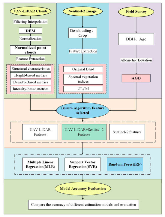
Figure 4.
Technology road map.
4. Results and Analyses
4.1. Importance Analysis and Screening of Characteristic Variables
Figure 5 shows the Z-scores of the identified LiDAR feature variables based on the Boruta algorithm, including four types of feature variables: stand canopy structure features, stand height features, LiDAR point cloud density features, and LiDAR intensity. As can be seen from the figure, all of the canopy structural characteristics of the forest stand in terms of canopy cover (CC), gap fraction (GF), and leaf area index (LAI) were selected. Eighteen feature variables were selected for the stand height feature, with high feature Z scores for cumulative height percentile AIH1, cumulative height percentile interquartile spacing AIHiq, height percentile interquartile spacing Hiq, and height percentile H1. Only one feature variable, D0, was selected from the point cloud density features. The point cloud intensity feature has eight feature variables selected, such as skewness (Iskew), kurtosis (Ikurt), and intensity percentiles I75 and I80.
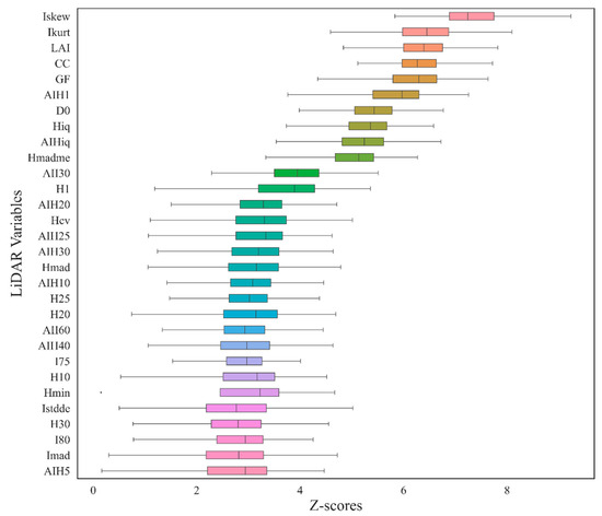
Figure 5.
Z-scores of the identified LiDAR feature variables.
A total of 30 features were chosen for the LiDAR-screened feature variables, out of which 18 features were selected for the stand height variable, accounting for 60% of all selected features, indicating that the stand height feature is an important variable reflecting the AGB of bamboo forests. Moreover, the Z scores of skewness (Iskew) and kurtosis (Ikurt) in stand intensity characteristics and canopy cover (CC), gap fraction (GF), and leaf area index (LAI) in stand canopy structure characteristics were ranked in the top five, which proved the high correlation with the AGB of the bamboo forest.
Figure 6 displays the Z-scores of the feature variables identified by Boruta’s algorithm for Sentinel-2. These variables encompass spectral bands, vegetation indices, and texture features such as blue, green, red, and near-infrared (NIR). One eigenvariable was chosen for the near-infrared band B8 in terms of raw spectral bands, while five eigenvariables were selected for vegetation indices based on their descending Z scores. These include differential vegetation index (DVI), soil-adjusted vegetation index (SAVI), triangular vegetation index (TVI), enhanced vegetation index (EVI), and vegetation attenuation index (PSRI). However, no eigenvariables were found to be significant for textural features.
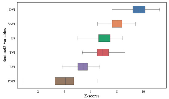
Figure 6.
Z-scores of the identified Sentinel-2 feature variables.
A total of six feature variables were chosen for the screening of Sentinel-2, and out of the twelve original spectral bands considered in the screening process, only one feature variable was selected within the near-infrared band. This selection highlights a strong correlation between the near-infrared band and the AGB (above-ground biomass) of bamboo forests. Additionally, among the twelve vegetation indices included in the screening, five distinct variables were identified as significant. These findings emphasize that vegetation indices such as DVI, SAVI, and TVI play a crucial role in reflecting the AGB of bamboo forests.
According to the analyses conducted, a total of 36 feature variables were chosen for the estimation of aboveground biomass (AGB) in bamboo forests. Among these variables, thirty were obtained from UAV-LiDAR data, while the remaining six were derived from Sentinel-2 data. The specific details can be found in Table 4.
Table 4.
Feature variables screened by Boruta’s algorithm.
4.2. Moso Bamboo Forest AGB Modelling Results
4.2.1. The MLR Model
Figure 7a–c illustrates the association between the estimated and observed AGB values using various remote sensing data sources as determined by the MLR model. As depicted in Figure 7, the MLR model developed using ST data exhibits a relatively lower R2 accuracy of merely 0.29 and a comparatively larger RMSE error of 4.24 Mg/hm2. In contrast, UL data follows with slightly improved performance, while the highest accuracy is achieved when combining UL + ST data. The AGB model accuracy, constructed using UL + ST data, exhibited a 155.17% increase compared with the R2 of single ST data and a 4.22% improvement over single UL data. This suggests that incorporating UL data, which reflects the structural characteristics of Moso bamboo forests, significantly enhances the precision of AGB estimation based on ST data. Certainly, considering an alternative viewpoint, the integration of ST data into UL data to capture the development of Moso bamboo forests, such as NDVI, SAVI, etc., has the potential to enhance the precision of estimating single UL data AGB to some degree.
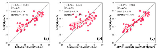
Figure 7.
The MLR model was employed to evaluate the relationship between estimated and measured AGB values of sample plots, utilizing a variety of remote sensing data sources.
4.2.2. The SVR Model
Figure 8a–c depict the correlation between predicted and measured AGB values using various remote sensing data sources, as estimated by the SVR model. It is evident from Figure 8 that the SVR model trained on ST data exhibits a relatively low R2 accuracy of only 0.16 and a higher RMSE error of 4.91 Mg/hm2 compared with UL data. However, when combining UL + ST data, the accuracy significantly improves. The AGB model constructed with UL + ST data demonstrates an R2 accuracy that is 418.75% higher than that of single ST data and 9.21% higher than single UL data, aligning with the findings of the MLR model analysis. Furthermore, considering both Figure 7 and Figure 8 together reveals that the SVR model’s R2 accuracy for UL and ST + UL models surpasses that of the MLR model, indicating superior performance in AGB estimation by the SVR approach compared with MLR modeling techniques.
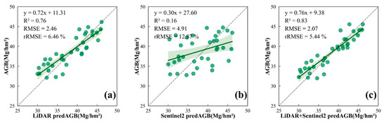
Figure 8.
The SVR model was employed to evaluate the relationship between estimated and measured AGB values of sample plots, utilizing a variety of remote sensing data sources.
4.2.3. The RF Model
Figure 9a–c depict the correlation between predicted and measured AGB values using various remote sensing data sources obtained from RF model estimation. It can be observed that the SVR model, based on ST data, exhibits a lower R2 accuracy of 0.45 and a larger RMSE error of 3.68 Mg/hm2 compared with UL data. However, when UL + ST data is utilized, the accuracy significantly improves with an R2 value of 0.89 and a high degree of model fit. The AGB model constructed using UL + ST data demonstrates a 97.78% higher accuracy than that solely relying on ST data in terms of R2, and it also outperforms the single UL data by 1.13%. This conclusion aligns with findings from MLR and SVR models as well. Furthermore, considering Figure 7, Figure 8 and Figure 9 collectively, it becomes evident that the RF model’s accuracy (measured by R2) surpasses both MLR and SVR models when utilizing three different types of data: UL, ST, and UL + ST. Notably for ST data specifically, the RF model achieves an improved estimation accuracy with an increase in R2 by 55.17% compared with the MLR model results and by 181.25% compared with the SVR model results, respectively, thus indicating its excellent performance in estimating AGB using diverse sources of input data.
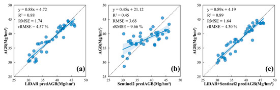
Figure 9.
The RF model was employed to evaluate the relationship between estimated and measured AGB values of sample plots, utilizing a variety of remote sensing data sources.
4.3. Comparative Evaluation of Outcomes in Estimating Aboveground Biomass (AGB)
Figure 10 shows the comparison of AGB estimation accuracy of different remote sensing data sources with different models
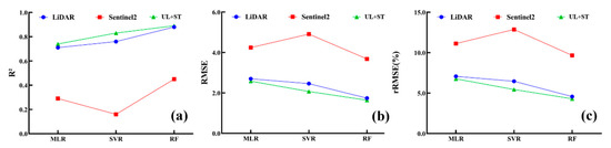
Figure 10.
Assessing the precision of AGB prediction models under varying circumstances.
4.3.1. Comparison of Different Modelling Approaches for the Same Data Source
The accuracy assessment of different schemes’ AGB estimation models is presented in Table 4. It can be observed that, for the UL data, MLR achieves an estimation accuracy R2 of 0.71, while SVR and RF attain R2 values of 0.76 and 0.88 for the nonparametric models, respectively. The results indicate that the estimation of LiDAR feature variables can be more precise when using the sample AGB with three different modeling methods. Among these methods, nonparametric models such as SVR and RF exhibit higher accuracy compared with parametric models such as MLR. Additionally, RF outperforms MLR in terms of accuracy, with an improvement of 7.04% and 23.94% in R2 values, respectively, while also achieving a lower root-mean-square error reduction of 8.89% and 35.56%, respectively.
Regarding ST data used for estimating bamboo forest aboveground biomass (AGB), it was observed that while the parametric modeling method MLR achieved an R-squared value (R2) of 0.29, the non-parametric models SVR and RF yielded respective R2 values of 0.16 and 0.45. These findings suggest that solely relying on Sentinel-2 characteristic variables does not lead to accurate estimations for bamboo forest AGB in either parametric or non-parametric models. Furthermore, there is a tendency towards significant overestimation at lower values while underestimating higher values becomes more pronounced. Nevertheless, when comparing with MLR results alone, employing the RF model demonstrates a notable improvement with a remarkable increase in R-squared value by 55.17% alongside a decrease in root mean square error (RMSE) by 13.21%. Consequently, this enhancement contributes to enhancing overall estimation accuracy to some degree.
When utilizing UL + ST data for estimating bamboo forest aboveground biomass (AGB), it was observed that a parametric modeling approach called MLR achieved an R-squared value of 0.74, while non-parametric models such as SVR and RF attained higher values at 0.83 and 0.89 correspondingly. This indicates that when combining LiDAR with Sentinel-2 data in various modeling techniques, it becomes possible to achieve favorable outcomes. The comparison between these approaches reveals that both nonparametric models (SVR and RF) outperform their parametric counterparts (MLR). Specifically, the R-squared values show improvements of approximately 12.16% and 20.27%, respectively. Moreover, the root-mean-square error demonstrates reductions of about 19.77% and 36.43%. In summary, the integration of LiDAR with Sentinel-2 for estimating bamboo forest AGB favors employing a non-parametric modeling technique, such as random forest (RF), which exhibits superior accuracy compared with support vector regression(SVR).
4.3.2. Comparison of Different Data Sources for the Same Modelling Approach
As indicated in Table 5, the non-parametric modeling approaches MLR and UL + ST data exhibit higher accuracy (R2) in estimating bamboo forest AGB compared with single UL data and ST data. Moreover, the estimation accuracy of UL data surpasses that of ST data. Similarly, the parametric models SVR and RF also demonstrate that the estimation accuracy of UL + ST data source is superior to that of only UL data. In contrast, the estimation accuracy of UL data remains higher than that of ST data. Additionally, it is observed that the model fit improves for these cases.
Table 5.
Accuracy evaluation of AGB estimation models for different scenarios.
5. Discussion
5.1. Feature Screening
Among the LiDAR characteristics examined in this investigation, stand height attributes constituted 60% and exhibited a significant importance score. This finding aligns with real-world observations, as well as previous research that has substantiated the pivotal role of height features in determining aboveground biomass (AGB). Cao Lin et al. [93] used small-spot full-waveform LiDAR data, extracted spatial information, and obtained the point cloud feature variables, the average height, and each stand feature. The correlation between them exhibited a strong association, with the tree height model demonstrating the highest level of accuracy. Among the canopy structural characteristics of the forest stand, canopy cover, gap fraction, and leaf area index emerged as the top five influential factors. Canopy cover (CC) serves as an indicator reflecting the density of the forest stand in general. AGB demonstrates a negative correlation with depression levels, whereby higher canopy cover impacts vegetation growth and light availability, consequently resulting in lower vegetation AGB [55]. The gap fraction (GF) affects the intensity of light received by vegetation under the canopy, which in turn affects the growth status of the vegetation [94]. The leaf area index (LAI) serves as a crucial factor in describing the physiological activities of forests, including photosynthesis, evapotranspiration, and the cycling of carbon and water within vegetation. A higher LAI indicates enhanced utilization of light energy by plants, leading to improved growth conditions and increased aboveground biomass (AGB). According to Zhang et al. [29], the incorporation of a canopy structure variable in the ULS-based AGB estimation model for urban forests resulted in enhanced accuracy in various models. Breast diameter estimation was conducted by Xiong et al. [95] using UAV-LiDAR to extract tree height and crown diameter, which were then utilized in a binary heteroscedastic growth equation for estimating the most suitable aboveground biomass (AGB) method for individual trees (R2 of 0.77, RMSE of 15.99 kg).
After being screened by Boruta, the intensity features skewness and kurtosis obtained the highest scores among all the feature variables. Brennan et al. [96] conducted an analysis of LiDAR data from eight regions regarding land class classification and discovered that incorporating the intensity feature resulted in a significant enhancement of 10–20% in classification accuracy. Antonarakis et al. [97] established kurtosis and skewness models based on LiDAR point elevations, which can effectively distinguish between artificially planted and naturally grown poplar riparian forests. To summarize, the Boruta technique offers improved comprehension of the impact that feature variables have on the dependent variable and efficiently identifies all relevant features associated with it from the original set.
Out of the various Sentinel-2 feature variables examined in the present investigation, only the NIR band and five vegetation indices (DVI, EVI, PSRI, SAVI, and TVI) were chosen. Du et al. [23] explored the correlation between Landsat Thematic Mapper (TM) data and AGB of Moso bamboo. They analyzed how Moso bamboo’s spectral reflectance and NDVI response relate to AGB. The findings also indicated that interpreting the AGB of Moso bamboo relies more on NIR and mid-infrared wavelengths rather than visible wavelengths. The correlation between the normalized vegetation index (NDVI) and Moso bamboo AGB was found to be weak. In contrast, the vertical vegetation index (PVI), enhanced vegetation index (EVI), and soil-adjusted vegetation index (SAVI) exhibited a significant correlation with Moso bamboo AGB. The R2 value of 0.48 indicated that EVI and SAVI were more effective in explaining variations in Moso bamboo AGB compared with NDVI. In this study, Boruta’s algorithm was employed for variable selection, which identified the near-infrared band (NIR) as one of the selected Sentinel-2 features. Chrysafis et al. [11] used Sentinel-2 images to estimate forest growth volume (GSV), and the research study showed that traditional vegetation indices such as NDVI did not improve the correlation intensity, while the differential vegetation index (DVI), enhanced vegetation index (EVI) and vertical vegetation index (PVI) had the strongest inversion intensity for GSV. As Steven et al. [98] pointed out, the vegetation indices of different satellite sensors cannot be directly equivalent. Theofanous et al. [13] used Sentinel-1 and Sentinel-2 time series data to simulate the AGB of Robinia pseudo acacia short-term rotation plantation in northeastern Greece. The research study showed that although NDVI was considered to have a strong correlation with AGB [99], the actual results did not identify NDVI as one of the vegetation indices with a high correlation with Robinia pseudo acacia AGB. Pertille et al. [100] used a Sentinel-1 active sensor and Sentinel-2 passive sensor to estimate the commercial wood yield of Korean pine plantations and established a stepwise regression model. The results showed that only the model fitting effect of the Sentinel-2 index was better, and the differential vegetation index (DVI) had the best correlation with Sentinel-2. Additionally, similar to previous studies, various vegetation indices such as DVI, EVI, and SAVI were utilized. These findings further validate the feasibility and reliability of Boruta’s algorithm for variable screening.
5.2. Analysis of Various Models in Comparison
The findings of this study demonstrate that both SVR and RF machine learning models exhibit superior performance compared with the MLR model, with RF outperforming SVR. MLR, being a statistical regression model, struggles to capture the complexity of extensive data, is sensitive to noise, and tends to suffer from underfitting issues, resulting in poor performance. On the other hand, RF effectively handles high-dimensional data while maintaining good noise immunity. During its operation, RF employs SVR to map the kernel function from low-dimensional to high-dimensional space. It subsequently solves non-linear problems in lower dimensions through linear regression hyperplanes. Although the SVR model fits training data well, it still requires optimization of penalty coefficients and gamma values for achieving an optimal model, which may potentially lead to overfitting. Feng et al. [101] compared the performance of linear, non-linear, RF, and SVR models in estimating vegetation AGB and found that the RF model exhibited superior results. According to a study conducted by Cao et al. [102], the RF model demonstrated superior accuracy in estimating forest biomass using satellite remote sensing compared with other models such as SVR, BPNN, KNN, and generalized linear mixed model (GLMM). The RF model demonstrated high accuracy in estimating forest structural parameters, as evidenced by a study conducted by Peng et al. [103] using UAV-LiDAR data to develop a model for assessing these parameters in tropical forests of China; Zhang Ya et al. [104] conducted a quantitative analysis of biomass using various models (SLR, LNN, BPNN, SVR, RF) in combination with LiDAR and high-resolution remote sensing imagery. The results indicated that the RF model demonstrated the highest level of accuracy in fitting (with an R2 value of 0.69 and RMSE of 26.98 Mg/ha). Zhou et al. [14] employed RF to estimate the biomass of urban ginkgo monocots using UAV-LiDAR data, resulting in accurate estimations. Furthermore, their findings provided evidence supporting the superiority of the RF model over alternative models in estimating AGB.
5.3. Comparative Analysis of Different Remote Sensing Data Sources
Different sensors have their own advantages. Optical satellite remote sensing, such as Sentinel-2, can monitor the growth of vegetation through spectral features, vegetation indices, and texture information; however, the presence of homoscedasticity or heteroscedasticity may result in the occurrence of underestimation and overestimation issues when estimating AGB in bamboo forests using ST data. The UAV-LiDAR point cloud data contains a large amount of forest 3D structural information, which can accurately separate the ground points and vegetation points and thus can obtain the forest vertical structure information that cannot be provided by Sentinel-2 remote sensing imagery. In a prior research study, Chen et al. provided evidence supporting LiDAR as the most precise data source for estimating aboveground biomass (AGB) [105]. This study also confirms that LiDAR provides reliable AGB prediction in bamboo forests using different modeling methods. The estimation accuracy was further improved by adding spectral information and vegetation index, thus proving that it is reasonable and valuable to synergize UAV-LiDAR and Sentinel-2 data sources to estimate AGB in bamboo forests.
6. Conclusions
In this study, we utilized the Moso bamboo forest located in Shanchuan Township, Zhejiang Province, China. We employed UAV-LiDAR (UL), Sentinel-2 (ST), and a combination of UL and ST as our data sources. Based on aboveground biomass surveys conducted in the Moso bamboo forests, we applied three models—MLR, SVR, and RF—to estimate the AGB of the forest. Our findings revealed that (1) the UL point cloud intensity and variables such as canopy cover (CC), gap fraction (GF), leaf area index (LAI), AIH1, AIHiq, and Hiq were significant indicators of Moso bamboo forest structure and AGB estimation. Similarly, vegetation indices such as DVI and SAVI from ST had a notable impact on estimating Moso bamboo forest AGB. (2) The accuracy of AGB estimation models constructed using UL was higher compared with those based solely on ST data. All three models achieved R2 values above 0.7, indicating high accuracy; RF, in particular, exhibited the highest accuracy with an R2 value of 0.88. (3) Combining ST with UL significantly improved the accuracy of AGB estimation for Moso bamboo forests using all three models when compared with using only ST data alone. For instance, when employing the RF model after combining UL + ST data, there was a remarkable improvement in AGB estimation accuracy by 97.7%, accompanied by a reduction in RMSE by 124.4%. Further analysis shows that the LiDAR data reflecting stand structure has an important impact on the AGB estimation of Moso bamboo forests, and UL + ST can significantly improve the accuracy of AGB estimation of Moso bamboo forests based on multispectral remote sensing data, which well solves the problem of low accuracy of AGB estimation due to the saturation of Canopy Cover of Moso bamboo forests with high optical remote sensing data.
7. Reflections and Outlook
In this study, Sentinel-2 data were combined with UAV-LiDAR data, the Boruta algorithm was used to screen remote sensing features, and Moso bamboo forest AGB was estimated based on MLR, SVR, and RF algorithms. Compared with previous studies, the accuracy was significantly improved by adding LiDAR feature variables, which proved that the combination of multispectral remote sensing data, which characterizes the spectral features of the forests, and LiDAR data, which reflects the structure of the stand, is a new way to estimate the AGB of Moso bamboo forest. This proves that the combination of multispectral remote sensing data characterizing forest spectral features and LiDAR data reflecting forest stand structure is a new way to estimate the AGB of the Moso bamboo forest. Meanwhile, there are some shortcomings in this study, which need to be explored and solved in the subsequent research.
- (1)
- In this study, three common models, MLR, SVR, and RF, were used to estimate the bamboo forest biomass, and more deep-learning models can be added to the estimation in future studies under the premise of expanding the sample capacity.
- (2)
- Limited by the flight range of the UAV-LiDAR, this study only explored the quantification of bamboo forest AGB based on the sample level, which can be expanded in future studies to explore the bamboo forest biomass and the changes in the time-space range.
- (3)
- The sample size of this study is limited, but it can be further expanded in future studies to investigate whether the modeling approach based on biomass range stratification can improve the estimation accuracy of AGB.
Author Contributions
L.Z.: Writing-original draft, Data curation, Methodology. Y.Z.: Data curation. C.C.: Data curation. X.L.: Data curation. F.M.: Data curation. L.L.: Data curation. J.Y.: Data curation. M.S.: Data curation. L.H.: Data curation. J.C.: Data curation. Z.Z.: Data curation. H.D.: Writing, review, and editing, Conceptualization, Funding acquisition, Supervision, Project administration. All authors have read and agreed to the published version of the manuscript.
Funding
The research was supported by the Science Technology Department of Zhejiang Province (No. 2023C02035), the National Natural Science Foundation of China (No. 32171785, 32201553), the Talent launching project of scientific research and development fund of Zhejiang A and F University (No. 2021LFR029).
Data Availability Statement
Data is contained within the article.
Conflicts of Interest
The authors declare that they have no known competing financial interests or personal relationships that could have appeared to influence the work reported in this study.
References
- Yen, T.-M.; Lee, J.-S. Comparing aboveground carbon sequestration between moso bamboo (Phyllostachys heterocycla) and China fir (Cunninghamia lanceolata) forests based on the allometric model. For. Ecol. Manag. 2011, 261, 995–1002. [Google Scholar] [CrossRef]
- Mciver, D.K.; Friedl, M.A. Using prior probabilities in decision-tree classification of remotely sensed data. Remote Sens. Environ. 2002, 81, 253–261. [Google Scholar] [CrossRef]
- Guo, Q.; Yang, G.; Du, T.; Shi, J. Carbon Character of Chinese Bamboo Forest. World Bamboo Ratt. 2005, 3, 4. [Google Scholar]
- Song, X.; Zhou, G.; Jiang, H.; Yu, S.; Fu, J.; Li, W.; Wang, W.; Ma, Z.; Peng, C. Carbon sequestration by Chinese bamboo forests and their ecological benefits: Assessment of potential, problems, and future challenges. Environ. Rev. 2011, 19, 418–428. [Google Scholar] [CrossRef]
- Nath, A.J.; Lal, R.; Das, A.K. Managing woody bamboos for carbon farming and carbon trading. Glob. Ecol. Conserv. 2015, 3, 654–663. [Google Scholar] [CrossRef]
- Miro, D.; Kim, C.; Hans, V.; Bert, G. Forest above-ground volume assessments with terrestrial laser scanning: A ground-truth validation experiment in temperate, managed forests. Ann. Bot. 2021, 6, 805–8119. [Google Scholar]
- Dong, L.; Du, H.; Mao, F.; Han, N.; Li, X.; Zhou, G.; Zhu, D.; Zheng, J.; Zhang, M.; Xing, L.; et al. Very High Resolution Remote Sensing Imagery Classification Using a Fusion of Random Forest and Deep Learning Technique—Subtropical Area for Example. IEEE J. Sel. Top. Appl. Earth Obs. Remote Sens. 2019, 13, 113–128. [Google Scholar] [CrossRef]
- Li, L.; Li, N.; Lu, D.; Chen, Y. Mapping Moso bamboo forest and its on-year and off-year distribution in a subtropical region using time-series Sentinel-2 and Landsat 8 data. Remote Sens. Environ. Interdiscip. J. 2019, 231, 111265. [Google Scholar] [CrossRef]
- Zhang, M.; Du, H.; Zhou, G.; Li, X.; Mao, F.; Dong, L.; Zheng, J.; Liu, H.; Huang, Z.; He, S. Estimating Forest Aboveground Carbon Storage in Hang-Jia-Hu Using Landsat TM/OLI Data and Random Forest Model. Forests 2019, 10, 1004. [Google Scholar] [CrossRef]
- Luo, K.; Wei, Y.; Du, J.; Liu, L.; Luo, X.; Shi, Y.; Pei, X.; Lei, N.; Song, C.; Li, J.; et al. Machine learning-based estimates of aboveground biomass of subalpine forests using Landsat 8 OLI and Sentinel-2B images in the Jiuzhaigou National Nature Reserve, Eastern Tibet Plateau. J. For. Res. 2022, 33, 1329–1340. [Google Scholar] [CrossRef]
- Chrysafis, I.; Mallinis, G.; Siachalou, S.; Patias, P. Assessing the relationships between growing stock volume and Sentinel-2 imagery in a Mediterranean forest ecosystem. Remote Sens. Lett. 2017, 8, 508–517. [Google Scholar] [CrossRef]
- Nuthammachot, N.; Askar, A.; Stratoulias, D.; Wicaksono, P. Combined use of Sentinel-1 and Sentinel-2 data for improving above-ground biomass estimation. Geocarto Int. 2022, 37, 366–376. [Google Scholar] [CrossRef]
- Theofanous, N.; Chrysafis, I.; Mallinis, G.; Domakinis, C.; Verde, N.; Siahalou, S. Aboveground Biomass Estimation in Short Rotation Forest Plantations in Northern Greece Using ESA’s Sentinel Medium-High Resolution Multispectral and Radar Imaging Missions. Forests 2021, 12, 902. [Google Scholar] [CrossRef]
- Zhou, L.; Li, X.; Zhang, B.; Xuan, J.; Gong, Y.; Tan, C.; Huang, H.; Du, H. Estimating 3D Green Volume and Aboveground Biomass of Urban Forest Trees by UAV-Lidar. Remote Sens. 2022, 14, 5211. [Google Scholar] [CrossRef]
- Wulder, M.A.; White, J.C.; Næsset, E.; Ørka, H.O.; Coops, N.C.; Hilker, T.; Bater, C.W.; Gobakken, T. LiDAR sampling for large-area forest characterization: A review. Remote Sens. Environ. 2012, 121, 196–209. [Google Scholar] [CrossRef]
- Li, X.; Du, H.; Mao, F.; Zhou, G.; Chen, L.; Xing, L.; Fan, W.; Xu, X.; Liu, Y.; Cui, L.; et al. Estimating bamboo forest aboveground biomass using EnKF-assimilated MODIS LAI spatiotemporal data and machine learning algorithms. Agric. For. Meteorol. 2018, 256–257, 445–457. [Google Scholar] [CrossRef]
- Ji, J.; Li, X.; Du, H.; Mao, F.; Fan, W.; Xu, Y.; Huang, Z.; Wang, J.; Kang, F. Multiscale leaf area index assimilation for Moso bamboo forest based on Sentinel-2 and MODIS data. Int. J. Appl. Earth Obs. Geoinf. 2021, 104, 102519. [Google Scholar] [CrossRef]
- Li, H.; Zhang, G.; Zhong, Q.; Xing, L.; Du, H. Prediction of Urban Forest Aboveground Carbon Using Machine Learning Based on Landsat 8 and Sentinel-2: A Case Study of Shanghai, China. Remote Sens. 2023, 15, 284. [Google Scholar] [CrossRef]
- Li, Y. Spatiotemporal Evolution of Bamboo Forest Carbon Storage and Response to Land Use Dynamic by Remote Sensing in Zhejiang Province; Zhejiang Agriculture & Forestry University: Hangzhou, China, 2018. [Google Scholar]
- Zhang, Y. Carbon Storage Estimation and Its Changes of Phyllostachys edulis Forests in Fujian Province; Chinese Academy of Foresty: Beijing, China.
- Cui, R.; Du, H.; Zhou, G.; Xu, X.; Dong, D.; Lu, Y. Remote sensing-based dynamic monitoring of moso bamboo forest and its carbon stock change in Anji County. J. Zhejiang A F Univ. 2011, 28, 10. [Google Scholar]
- Li, Y.; Han, N.; Li, X.; Du, H.; Mao, F.; Cui, L.; Liu, T.; Xing, L. Spatiotemporal Estimation of Bamboo Forest Aboveground Carbon Storage Based on Landsat Data in Zhejiang, China. Remote Sens. 2018, 10, 898. [Google Scholar] [CrossRef]
- Du, H.; Cui, R.; Zhou, G.; Shi, Y.; Xu, X.; Fan, W.; Lü, Y. The responses of Moso bamboo (Phyllostachys heterocycla var. pubescens) forest aboveground biomass to Landsat TM spectral reflectance and NDVI. Acta Ecol. Sin. 2010, 30, 257–263. [Google Scholar] [CrossRef]
- Du, H.; Zhou, G.; Ge, H.; Fan, W.; Xu, X.; Fan, W.; Shi, Y. Satellite-based carbon stock estimation for bamboo forest with a non-linear partial least square regression technique. Int. J. Remote Sens. 2011, 33, 1917–1933. [Google Scholar] [CrossRef]
- Chen, Y.; Li, L.; Lu, D.; Li, D. Exploring Bamboo Forest Aboveground Biomass Estimation Using Sentinel-2 Data. Remote Sens. 2019, 11, 7. [Google Scholar] [CrossRef]
- Dengsheng, L. The potential and challenge of remote sensing-based biomass estimation. Int. J. Remote Sens. 2006, 27, 1297–1328. [Google Scholar]
- Galidaki, G.; Zianis, D.; Gitas, I.; Radoglou, K.; Karathanassi, V.; Tsakiri–Strati, M.; Woodhouse, I.; Mallinis, G. Vegetation biomass estimation with remote sensing: Focus on forest and other wooded land over the Mediterranean ecosystem. Int. J. Remote Sens. 2016, 38, 1940–1966. [Google Scholar] [CrossRef]
- García, M.; Riaño, D.; Chuvieco, E.; Danson, F.M. Estimating biomass carbon stocks for a Mediterranean forest in central Spain using LiDAR height and intensity data. Remote Sens. Environ. 2010, 114, 816–830. [Google Scholar] [CrossRef]
- Zhang, B.; Li, X.; Du, H.; Zhou, G.; Mao, F.; Huang, Z.; Zhou, L.; Xuan, J.; Gong, Y.; Chen, C. Estimation of Urban Forest Characteristic Parameters Using UAV-Lidar Coupled with Canopy Volume. Remote Sens. 2022, 14, 6375. [Google Scholar] [CrossRef]
- Cao, L.; Coops, N.C.; Sun, Y.; Ruan, H.; Wang, G.; Dai, J.; She, G. Estimating canopy structure and biomass in bamboo forests using airborne LiDAR data. ISPRS J. Photogramm. Remote Sens. 2019, 148, 114–129. [Google Scholar] [CrossRef]
- Lu, D.; Chen, Q.; Wang, G.; Liu, L.; Li, G.; Moran, E. A survey of remote sensing-based aboveground biomass estimation methods in forest ecosystems. Int. J. Digit. Earth 2014, 9, 63–105. [Google Scholar] [CrossRef]
- Laurin, G.V.; Chen, Q.; Lindsell, J.A.; Coomes, D.A.; Frate, F.D.; Guerriero, L.; Pirotti, F.; Valentini, R. Above ground biomass estimation in an African tropical forest with lidar and hyperspectral data. ISPRS J. Photogramm. Remote Sens. 2014, 89, 49–58. [Google Scholar] [CrossRef]
- Rana, P.; Popescu, S.; Tolvanen, A.; Gautam, B.; Srinivasan, S.; Tokola, T. Estimation of tropical forest aboveground biomass in Nepal using multiple remotely sensed data and deep learning. Int. J. Remote Sens. 2023, 44, 5147–5171. [Google Scholar] [CrossRef]
- Wang, Y.; Jia, X.; Chai, G.; Lei, L.; Zhang, X. Improved estimation of aboveground biomass of regional coniferous forests integrating UAV-LiDAR strip data, Sentinel-1 and Sentinel-2 imageries. Plant Methods 2023, 19, 65. [Google Scholar] [CrossRef] [PubMed]
- Jiang, F.; Deng, M.; Tang, J.; Fu, L.; Sun, H. Integrating spaceborne LiDAR and Sentinel-2 images to estimate forest aboveground biomass in Northern China. Carbon Balance Manag. 2022, 17, 12. [Google Scholar] [CrossRef] [PubMed]
- Wang, J.; Du, H.; Li, X.; Mao, F.; Kang, F. Remote Sensing Estimation of Bamboo Forest Aboveground Biomass Based on Geographically Weighted Regression. Remote Sens. 2021, 13, 2962. [Google Scholar] [CrossRef]
- Rosas-Chavoya, M.; López-Serrano, P.M.; Vega-Nieva, D.J.; Hernández-Díaz, J.C.; Wehenkel, C.; Corral-Rivas, J.J. Estimating Above-Ground Biomass from Land Surface Temperature and Evapotranspiration Data at the Temperate Forests of Durango, Mexico. Forests 2023, 14, 299. [Google Scholar] [CrossRef]
- Yukun, G.; Dengsheng, L.; Guiying, L.; Guangxing, W.; Qi, C.; Lijuan, L.; Dengqiu, L. Comparative Analysis of Modeling Algorithms for Forest Aboveground Biomass Estimation in a Subtropical Region. Remote Sens. 2018, 10, 627. [Google Scholar]
- Kursa, M.B.; Rudnicki, W.R. Feature Selection with the Boruta Package. J. Stat. Softw. 2010, 36, 85. [Google Scholar] [CrossRef]
- Kursa, M.B.; Rudnicki, W.R. Boruta: Wrapper Algorithm for All Relevant Feature Selection. 2015. Available online: https://cran.r-project.org/web/packages/Boruta/index.html (accessed on 14 February 2024).
- Mostofa, M.Z. Comparing Prediction Accuracies of Cancer Survival Using Machine Learning Techniques and Statistical Methods in Combination with Data Reduction Methods; North Dakota State University of Agriculture and Applied Science: Fargo, ND, USA, 2022. [Google Scholar]
- Zhao, H.L.; Gan, S.; Yuan, X.P.; Hu, L.; Wang, J.J.; Liu, S. Prediction of low Zn concentrations in soil from mountainous areas of central Yunnan Province using a combination of continuous wavelet transform and Boruta algorithm. Int. J. Remote Sens. 2023, 44, 4753–4774. [Google Scholar] [CrossRef]
- Gilani, N.; Belaghi, R.A.; Aftabi, Y.; Faramarzi, E.; Edgünlü, T.; Somi, M.H. Identifying Potential miRNA Biomarkers for Gastric Cancer Diagnosis Using Machine Learning Variable Selection Approach. Front. Genet. 2022, 12, 779455. [Google Scholar] [CrossRef]
- Uniyal, S.; Purohit, S.; Chaurasia, K.; Rao, S.S.; Amminedu, E. Quantification of carbon sequestration by urban forest using Landsat 8 OLI and machine learning algorithms in Jodhpur, India. Urban For. Urban Green. 2022, 67, 127445. [Google Scholar] [CrossRef]
- Huang, T.; Ou, G.; Wu, Y.; Zhang, X.; Liu, Z.; Xu, H.; Xu, X.; Wang, Z.; Xu, C. Estimating the Aboveground Biomass of Various Forest Types with High Heterogeneity at the Provincial Scale Based on Multi-Source Data. Remote Sens. 2023, 15, 3550. [Google Scholar] [CrossRef]
- Englhart, S.; Keuck, V.; Siegert, F. Modeling Aboveground Biomass in Tropical Forests Using Multi-Frequency SAR Data—A Comparison of Methods. IEEE J. Sel. Top. Appl. Earth Obs. Remote Sens. 2012, 5, 298–306. [Google Scholar] [CrossRef]
- Monnet, J.-M.; Chanussot, J.; Berger, F. Support Vector Regression for the Estimation of Forest Stand Parameters Using Airborne Laser Scanning. IEEE Geosci. Remote Sens. Lett. 2011, 8, 580–584. [Google Scholar] [CrossRef]
- Tamiminia, H.; Salehi, B.; Mahdianpari, M.; Beier, C.M.; Johnson, L. Mapping Two Decades of New York State Forest Aboveground Biomass Change Using Remote Sensing. Remote Sens. 2022, 14, 4097. [Google Scholar] [CrossRef]
- Yu, Y.; Pan, Y.; Yang, X.; Fan, W. Spatial Scale Effect and Correction of Forest Aboveground Biomass Estimation Using Remote Sensing. Remote Sens. 2022, 14, 2828. [Google Scholar] [CrossRef]
- Zhang, L.; Zhang, X.; Shao, Z.; Jiang, W.; Gao, H. Integrating Sentinel-1 and 2 with LiDAR data to estimate aboveground biomass of subtropical forests in northeast Guangdong, China. Int. J. Digit. Earth 2023, 16, 158–182. [Google Scholar] [CrossRef]
- Dong, L.; Du, H.; Han, N.; Li, X.; Zhu, D.; Mao, F.; Zhang, M.; Zheng, J.; Liu, H.; Huang, Z.; et al. Application of Convolutional Neural Network on Lei Bamboo Above-Ground-Biomass (AGB) Estimation Using Worldview-2. Remote Sens. 2020, 12, 958. [Google Scholar] [CrossRef]
- Liu, H.; Zhang, Z.; Cao, L. Estimating forest stand characteristics in a coastal plain forest plantation based on vertical structure profile parameters derived from ALS data. J. Remote Sens. 2018, 22, 17. [Google Scholar] [CrossRef]
- Zhao, X.; Guo, Q.; Su, Y.; Xue, B. Improved progressive TIN densification filtering algorithm for airborne LiDAR data in forested areas. ISPRS J. Photogramm. Remote Sens. 2016, 117, 79–91. [Google Scholar] [CrossRef]
- Guomo, Z. Study on Carbon Storage, Fixation and Its Allocation and Distribution in Moso Bamboo Forest Ecosystems; Zhejiang University: Hangzhou, China, 2006. [Google Scholar]
- Ma, Q.; Su, Y.; Guo, Q. Comparison of Canopy Cover Estimations From Airborne LiDAR, Aerial Imagery, and Satellite Imagery. IEEE J. Sel. Top. Appl. Earth Obs. Remote Sens. 2017, 10, 4225–4236. [Google Scholar] [CrossRef]
- Liu, K.; Shen, X.; Cao, L.; Wang, G.; Cao, F. Estimating forest structural attributes using UAV-LiDAR data in Ginkgo plantations. ISPRS J. Photogramm. Remote Sens. 2018, 146, 465–482. [Google Scholar] [CrossRef]
- Camarretta, N.; Ehbrecht, M.; Seidel, D.; Wenzel, A.; Zuhdi, M.; Merk, M.S.; Schlund, M.; Erasmi, S.; Knohl, A. Using Airborne Laser Scanning to Characterize Land-Use Systems in a Tropical Landscape Based on Vegetation Structural Metrics. Remote Sens. 2021, 13, 4794. [Google Scholar] [CrossRef]
- Estornell, J.; Hadas, E.; Martí, J.; López-Cortés, I. Tree extraction and estimation of walnut structure parameters using airborne LiDAR data. Int. J. Appl. Earth Obs. Geoinf. 2021, 96, 102273. [Google Scholar] [CrossRef]
- Dong, W.; Lan, J.; Liang, S.; Yao, W.; Zhan, Z. Selection of LiDAR geometric features with adaptive neighborhood size for urban land cover classification. Int. J. Appl. Earth Obs. Geoinf. 2017, 60, 99–110. [Google Scholar] [CrossRef]
- Owers, C.J.; Rogers, K.; Woodroffe, C.D. Terrestrial laser scanning to quantify above-ground biomass of structurally complex coastal wetland vegetation. Estuar. Coast. Shelf Sci. 2018, 204, 164–176. [Google Scholar] [CrossRef]
- Michalowska, M.; Rapinski, J. A Review of Tree Species Classification Based on Airborne LiDAR Data and Applied Classifiers. Remote Sens. 2021, 13, 353. [Google Scholar] [CrossRef]
- Francisca, R.D.S.P.; Milton, K.; Mário, G.S.; Gustavo, E.; Cristina, B.; Gregoire, V. Reducing Uncertainty in Mapping of Mangrove Aboveground Biomass Using Airborne Discrete Return Lidar Data. Remote Sens. 2018, 10, 637. [Google Scholar]
- Shi, Y.; Wang, T.; Skidmore, A.K.; Heurich, M. Important LiDAR metrics for discriminating forest tree species in Central Europe. ISPRS J. Photogramm. Remote Sens. 2018, 137, 163–174. [Google Scholar] [CrossRef]
- Tucker, C.; Elgin, J.; McMurtrey, J.; Fan, C. Monitoring corn and soybean crop development with hand-held radiometer spectral data. Remote Sens. Environ. 1979, 8, 237–248. [Google Scholar] [CrossRef]
- Jiang, Z.; Huete, A.R.; Didan, K.; Miura, T. Development of a two-band enhanced vegetation index without a blue band. Remote Sens. Environ. 2008, 112, 3833–3845. [Google Scholar] [CrossRef]
- Broge, N.H.; Leblanc, E. Comparing prediction power and stability of broadband and hyperspectral vegetation indices for estimation of green leaf area index and canopy chlorophyll density. Remote Sens. Environ. 2001, 76, 156–172. [Google Scholar] [CrossRef]
- Tan, Y.; Sun, J.-Y.; Zhang, B.; Chen, M.; Liu, Y.; Liu, X.-D. Sensitivity of a Ratio Vegetation Index Derived from Hyperspectral Remote Sensing to the Brown Planthopper Stress on Rice Plants. Sensors 2019, 19, 375. [Google Scholar] [CrossRef] [PubMed]
- Merzlyak, M.N.; Gitelson, A.A.; Chivkunova, O.B.; Rakitin, V.Y. Non-destructive optical detection of pigment changes during leaf senescence and fruit ripening. Physiol. Plant. 1999, 106, 135–141. [Google Scholar] [CrossRef]
- Chen, D.; Huang, J.; Jackson, T.J. Vegetation water content estimation for corn and soybeans using spectral indices derived from MODIS near- and short-wave infrared bands. Remote Sens. Environ. 2005, 98, 225–236. [Google Scholar] [CrossRef]
- Rouse, E.B.; Coops, N.C.; St-Onge, B.; Begin, J. Estimating Forest Stand Age from LiDAR-Derived Predictors and Nearest Neighbor Imputation. For. Sci. 2014, 60, 128–136. [Google Scholar]
- Rouse, J.W.; Haas, R.H.; Schell, J.A.; Deering, D.W. Monitoring Vegetation Systems in the Great Plains with Erts. NASA Spec. Publ. 1974, 351, 309. [Google Scholar]
- Qiu, M.; Gan, S.; Zhao, L. Watershed Extraction in the Erhai Sea using Sentinel-2 Imagery An Analytical Study of Index Methods. Urban Geotech. Investig. Surv. 2022, 11, 117–122. [Google Scholar]
- Huete, A.R. A soil-adjusted vegetation index (SAVI). Remote Sens. Environ. 1988, 25, 295–309. [Google Scholar] [CrossRef]
- Muhaimin, M.; Fitriani, D.; Adyatma, S.; Arisanty, D. mapping build-up area density using normalized difference built-up index (ndbi) and urban index (ui) wetland in the city banjarmasin. IOP Conf. Ser. Earth Environ. Sci. 2022, 1089, 012036. [Google Scholar] [CrossRef]
- Gitelson, A.A.; Gritz, Y.; Merzlyak, M.N. Relationships between leaf chlorophyll content and spectral reflectance and algorithms for non-destructive chlorophyll assessment in higher plant leaves. J. Plant Physiol. 2003, 160, 271–282. [Google Scholar] [CrossRef]
- Mohammadpour, P.; Viegas, D.X.; Viegas, C.J.R.S. Vegetation Mapping with Random Forest Using Sentinel 2 and GLCM Texture Feature—A Case Study for Lousã Region, Portugal. Remote Sens. 2022, 14, 4585. [Google Scholar] [CrossRef]
- Iqbal, N.; Mumtaz, R.; Shafi, U.; Zaidi, S.M.H. Gray level co-occurrence matrix (GLCM) texture based crop classification using low altitude remote sensing platforms. PeerJ Comput. Sci. 2021, 7, e536. [Google Scholar] [CrossRef] [PubMed]
- Marshall, T.L.; Nickels, L.C.; Brady, P.W.; Edgerton, E.J.; Lee, J.J.; Hagedorn, P.A. Developing a machine learning model to detect diagnostic uncertainty in clinical documentation. J. Hosp. Med. 2023, 18, 405–412. [Google Scholar] [CrossRef] [PubMed]
- Lamine, G.M.; Hilal, K.M.; Rongqin, C.; Fei, L. Potential of Vis-NIR to measure heavy metals in different varieties of organic-fertilizers using Boruta and deep belief network. Ecotoxicol. Environ. Saf. 2021, 228, 112996. [Google Scholar]
- Lumley, T.; Miller, A. leaps: Regression Subset Selection. EMBO J. 2009, 7. [Google Scholar]
- Ding, j.; Huang, w.; Liu, y.; Hu, y. Estimation of Forest Aboveground Biomass in Northwest Hunan Province Based on Machine Learning and Multi-Source Data. Sci. Silvae Sin. 2021, 57, 36–48. [Google Scholar]
- Poorazimy, M.; Shataee, S.; McRoberts, R.E.; Mohammadi, J. Integrating airborne laser scanning data, space-borne radar data and digital aerial imagery to estimate aboveground carbon stock in Hyrcanian forests, Iran. Remote Sens. Environ. 2020, 240, 111669. [Google Scholar] [CrossRef]
- Zhao, X. A Study on Forest Aboveground Biomass Estimation Based on Airborne Excitation Radar; Xi’an University of Science and Technology: Xi’an, China, 2020. [Google Scholar]
- Xiao, Y. Research on the Estimation Method of Forest Volume of Wangyedian Forest Farm Based on Multi-Source Remote Sensing Data; Central South University of forestry & Technology: Changsha, China, 2021. [Google Scholar]
- Breiman, L. Random Forests. Mach. Learn. 2001, 45, 148–156. [Google Scholar]
- Breiman, L. Bagging Predictors. Mach. Learn. 1996, 24, 123–140. [Google Scholar] [CrossRef]
- Ho, T.K. The Random Subspace Method for Constructing Decision Forests. IEEE Trans. Pattern Anal. Mach. Intell 1998, 20, 832–844. [Google Scholar]
- Tang, S. Study on Extraction of Stand Age Information of Typical Coniferous Forests in Northeast China and Its Impact on Tree Species Classification; Nanjing University: Nanjing, China, 2020. [Google Scholar]
- Dong, S.; Huang, Z. A Brief Theoretical Overview of Random Forests. J. Integr. Technol. 2013, 2, 1–7. [Google Scholar]
- Kuangnan, F.; Jianbin, W.; Jianpin, Z.; Bangchang, X. A Review of Research on Random Forest Methods. Stat. Inf. Forum 2011, 26, 32–38. [Google Scholar]
- Chen, L.; Zhou, G.; Du, H.; Liu, Y.; Mao, F.; Xu, X.; Li, X.; Cui, L.; Li, Y.; Zhu, D. Simulation of CO2 Flux and Controlling Factors in Moso Bamboo Forest Using Random Forest Algorithm. Sci. Silvae Sin. 2018, 54, 1–12. [Google Scholar]
- Wen, B.; Zhao, L.; Huang, L. Proof of Asymptotic Equivalence by Cross-Validation of the AIC Criterion with the Leave-One-Out Method. Stat. Decis. 2022, 38, 40–43. [Google Scholar] [CrossRef]
- Lin, C.; Nicholas, C.; Txomin, H.; John, I.; Jinsong, D.; Guanghui, S. Using Small-Footprint Discrete and Full-Waveform Airborne LiDAR Metrics to Estimate Total Biomass and Biomass Components in Subtropical Forests. Remote Sens. 2014, 6, 7110–7135. [Google Scholar]
- Richardson, J.J.; Moskal, L.M.; Kim, S.H. Modeling approaches to estimate effective leaf area index from aerial discrete-return LIDAR. Agric. For. Meteorol. 2009, 149, 1152–1160. [Google Scholar] [CrossRef]
- Xiong, F.; Zeng, H.; Xie, J.; Li, X.; Chen, J. Preliminary study on dry and wet season changes of biomass on Chinese fir forest land based on UAVLidar. Natl. Remote Sens. Bull. 2023, 1–13. [Google Scholar] [CrossRef]
- Brennan, R.; Webster, T.L. Object-oriented land cover classification of lidar-derived surfaces. Can. J. Remote Sens. 2006, 32, 162–172. [Google Scholar] [CrossRef]
- Antonarakis, A.S.; Richards, K.S.; Brasington, J. Object-based land cover classification using airborne LiDAR. Remote Sens. Environ. 2008, 112, 2988–2998. [Google Scholar] [CrossRef]
- Steven, M.D.; Malthus, T.J.; Baret, F.; Xu, H.; Chopping, M.J. Intercalibration of vegetation indices from different sensor systems. Remote Sens. Environ. 2003, 88, 412–422. [Google Scholar] [CrossRef]
- Zhu, X.; Liu, D. Improving forest aboveground biomass estimation using seasonal Landsat NDVI time-series. ISPRS J. Photogramm. Remote Sens. 2015, 102, 222–231. [Google Scholar] [CrossRef]
- Pertille, C.T.; Nicoletti, M.F.; Dobner Jr, M. Estimating the commercial volume of a Pinus taeda L. plantation using active and passive sensors. Cerne 2023, 29, e-013108. [Google Scholar] [CrossRef]
- Feng, Y.; Lu, D.; Chen, Q.; Keller, M.; Moran, E.; Nara Dos-Santos, M.; Luis Bolfe, E.; Batistella, M. Examining effective use of data sources and modeling algorithms for improving biomass estimation in a moist tropical forest of the Brazilian Amazon. Int. J. Digit. Earth 2017, 10, 996–1016. [Google Scholar] [CrossRef]
- Luodan, C.; Jianjun, P.; Ruijuan, L.; Jialin, L.; Zhaofu, L. Integrating Airborne LiDAR and Optical Data to Estimate Forest Aboveground Biomass in Arid and Semi-Arid Regions of China. Remote Sens. 2018, 10, 532. [Google Scholar]
- Peng, X.; Zhao, A.; Chen, Y.; Chen, Q.; Liu, H.; Wang, J.; Li, H. Comparison of Modeling Algorithms for Forest Canopy Structures Based on UAV-LiDAR: A Case Study in Tropical China. Forests 2020, 11, 1324. [Google Scholar] [CrossRef]
- Zang, Y.; Shao, Z. Assessing of Urban Vegetation Biomass in Combination with LiDAR and High-resolution Remote Sensing Images. Int. J. Remote Sens. 2021, 42, 964–985. [Google Scholar] [CrossRef]
- Chen, Q. LiDAR Remote Sensing of Vegetation Biomass. Environ. Sci. 2013, 399, 399–420. [Google Scholar]
Disclaimer/Publisher’s Note: The statements, opinions and data contained in all publications are solely those of the individual author(s) and contributor(s) and not of MDPI and/or the editor(s). MDPI and/or the editor(s) disclaim responsibility for any injury to people or property resulting from any ideas, methods, instructions or products referred to in the content. |
© 2024 by the authors. Licensee MDPI, Basel, Switzerland. This article is an open access article distributed under the terms and conditions of the Creative Commons Attribution (CC BY) license (https://creativecommons.org/licenses/by/4.0/).