Abstract
Forest biomass is expected to remain a key part of the national energy portfolio mix, yet residual forest biomass is currently underused. This study aimed to estimate the potential availability of waste woody biomass in the Aizu region and its energy potential for local bioelectricity generation as a sustainable strategy. The results showed that the available quantity of forest residual biomass for energy production was 191,065 tons, with an average of 1.385 t/ha in 2018, of which 72% (146,976 tons) was from logging residue for commercial purposes, and 28% (44,089 tons) was from thinning operations for forest management purposes. Forests within the biomass–collection radius of a local woody power plant can provide 45,925 tons of residual biomass, supplying bioelectricity at 1.6 times the plant’s capacity, which could avoid the amount of 65,246 tons of CO2 emission per year by replacing coal-fired power generation. The results highlight the bioelectricity potential and carbon-neutral capacity of residual biomass. This encourages government initiatives or policy inclinations to sustainably boost the production of bioenergy derived from residual biomass.
1. Introduction
Energy represents a cornerstone in social development and economic growth by providing fundamental modern services for fulfilling basic social needs, driving economic growth, and fueling human development [1]. The longstanding global dependence on fossil fuels has led to pressing concerns such as air pollution, greenhouse gas emissions, and the formation of a “carbon bubble” [2,3,4]. As the world shifts away from fossil fuels, renewable energy (particularly woody biomass) emerges as a promising alternative after wind, solar, and geothermal technologies’ market penetration [3,4,5,6]. Unlike the variable outputs of solar and wind power due to their fluctuation with weather and season [7], biomass offers consistent energy production throughout the year, positioning it as a reliable base load power source. This stability, combined with its ability to balance the intermittency of other renewables, underscores the potential of biomass in creating a diversified, sustainable energy system [8,9].
In Japan, 88% of the country’s 2019 total primary energy supply relied on fossil fuels, and they heavily depend on imports to meet energy demands [10,11]. As coal is the most carbon-intensive fossil fuel and accounts for 31.6% of Japan’s total power generation [12], transitioning to renewables is not just environmentally beneficial but also crucial for Japan’s 2050 carbon neutrality goal. To accelerate this transition, policies like the feed-in tariff policy have been implemented, promoting coal-fired projects integrating renewable energy since 2012 [5,13]. A total of 307 power generation plants have adopted, or are planning to adopt, biomass co-firing energy resources to phase out coal in the power sector.
A total of 67% of Japan’s total land area is covered by forests, and 41% of the country’s forests are mature post-WWII-planted forests (primarily Japanese cedar (44%) and Japanese cypress (25%)) featuring fast growth and construction suitability [14]. The majority of forest resources have been utilized for papermaking, building, and furniture industries. Residues from lumber (processed wood ready for housing construction or furniture making) preparation or thinning are the main woody fuel resource for power generation [15]. Current wood consumption for electricity is low, accounting for 0.058% of the total wood supply [16]. Challenges like labor shortages, high management and collection costs, and competition with other sectors have hindered optimal utilization of forest residues and often led to the abandonment of residues in the thinning site or landing field [14,17,18,19,20,21,22]. Other reasons that have hindered the expansion of woody biomass for biomass energy include the high initial investment for facilities, fuelwood procurement, transportation costs, lower energy conversion efficiency (25–30%), source competition with other sectors, and a general decrease across the entire domestic forestry industry affected by the import of cheaper foreign timber products (70% of Japan’s total wood supply and 30.7% of fuel wood are imported) [5,16,23,24]. Life-cycle studies on energy consumption and greenhouse gas emissions indicate that substituting fossil fuels with forest residues and fast-growing woods may promote carbon neutrality [25,26]. Tapping into the potential of forest residues could enhance Japan’s domestic energy supplies and reduce fossil fuel reliance, making it imperative to assess their quantity, distribution, and bioelectricity conversion potential. Such data would serve as an important reference for sustainable forest management practices and appropriate strategies to promote renewable energy and revitalize rural society [27,28].
Japan has a long tradition of research into forest biomass and its associated energy utilization, including the estimation of availability, energy supply potential, cost estimation, and technical/economic feasibility [7,18,20,29,30,31,32]. There are studies focusing on forest residues, however they remain in the minority. Moreover, many of them estimated logging residue availability based on the existing forest register book (GIS format) which can be updated every several years. The most used GIS data provided by the New Energy and Industrial Technology Development Organization (2011) features a coarse resolution (1 km2) and the estimations rely on decade-old data, limiting their applicability to smaller-scale regions [33]. Thus, up-to-date forest information and a fine-resolution forest map that enables the classification of detailed tree types from advanced remote sensing images are essential for reflecting field conditions, estimating forest biomass, and conducting economic analysis to achieve more sustainable and efficient forest resource management [34,35,36].
The evolution of satellite remote sensing technology has revolutionized the methods used to observe the land surface. Sentinel-2 stands out for its free-of-charge, fine spatial and temporal resolution, as well as the availability of a red-edge band, achieving higher accuracies compared to images from other medium-resolution satellites [8,25]. Sentinel-2 multispectral satellite products were provided by a joint effort of the European Space Agency (ESA) and the European Union (EU) [37]. Sentinel-2 features 13 multispectral bands and provides fine-resolution (10–60 m) imagery for land cover/use monitoring [38]. Furthermore, GIS methods have become powerful tools for analyzing, visualizing, and interpreting spatial data. The combination of remote sensing, GIS, and ground-based measurements enables a comprehensive and accurate approach for monitoring and evaluating land surfaces, and it has become prevalent in estimating above-ground biomass (AGB) [39,40,41,42,43,44,45,46,47,48].
This study aimed to estimate the availability and energy potential of forest residual biomass derived from thinning and logging activities for electricity generation in the Aizu region of Fukushima for local bioelectricity generation. To do this, residual biomass was estimated based on local forest management practices and a high-resolution forest map extracted from multi-temporal Sentinel-2A images [49]. Road density data was used to filter the availability of residuals for transportation, and the corresponding potential for bioelectricity supply was determined. As there are hundreds of woody biomass power plants that are either operational or planned to be in operation in Japan, we believe that this paper will serve as a valuable reference for informing decision makers as well as those planning or operating woody biomass plants by assessing the potential of residual biomass energy, practicing sustainable forest management (health and harvest), providing guidance to evaluate coal displacement opportunities [27,50].
2. Materials and Methods
2.1. Study Area
Aizu region is located in western Fukushima Prefecture (Figure 1, 36°54′N to 37°50′N and 139°10′E to 140°17′E). The area covers nearly 542,069 ha, which accounts for 39% of Fukushima Prefecture. Administratively, it consists of two cities, eleven towns, and four villages in order of administrative ranking. The average temperature of the warmest month (August) exceeds 20 °C, and the coldest month (January) is below −2.03 °C. The annual precipitation is nearly 1715.6 mm. The average wind speed is 1.4 m/s [51].
Forests covered nearly 415,666 ha in 2010, accounting for 44% of the total forest area of Fukushima Prefecture [52]. The Aizu region has the highest number, accounting for 33% of Fukushima’s total whole tree volume [52]. In 2013, the Aizu region accounted for 14% of the prefecture’s total felling and bucking, and its forest industry contributed 0.08% of the prefecture’s total gross domestic product [53].

Figure 1.
Location of the Fukushima Prefecture (left), and SRTM DEM map (U.S. Geological Survey, 2013 [54]) of Aizu region (right).
The forest is divided into state (40.1% of its total area) and private (59.9% of its total area) forests [52]. In the region’s private forest, sawtooth oak (Quercus acutissima) and jolcham oak (Quercus serrata) are the major broad-leaved species, whereas Japanese cedar (Cryptomeria japonica) and Hinoki cypress (Chamaecyparis obtusa) are the major needle-leaved species [52]. Natural forests are dominated by broad-leaved species such as the Japanese beech (Fagus crenata) and the Japanese mizunara oak (Quercus crispula Blume), whereas Japanese cedar (Cryptomeria japonica) and Japanese larch (Larix kaempferi) are the major needle-leaved species dominating the artificial forest.
2.2. Data Preprocessing and Classification
Sentinel-2A products were used to generate a forest map of the Aizu region. Fifty-one images of Sentinel-2A were acquired from 2018 to 2020 through the online cloud platform Google Earth Engine (GEE) (https://earthengine.google.org, accessed on 23 February 2021). The Sentinel-2A data is already applied with atmospheric correction. The overall methodology used for processing Sentinel-2A images in this study is shown in Figure 2. Initially, within the GEE code editor (https://code.earthengine.google.com/, accessed on), cloud cover filter was utilized and set for a cloud coverage of less than 10% to remove the clouds. A median composition method (by taking the median of each cloud-free pixel available) was performed to composite cloud-free images and cover the entire study area. This method enables the minimization of potential distortions from seasonal or short-term environmental variations [55]. The periods during which the images were acquired were categorized into three seasons: (1) spring (April–May), when broad-leaf trees start to green up; (2) summer (June–August), when forested areas reach peak greenness; (3) autumn (October–November), when some leaves start to gradually change colors. Among the 51 scenes acquired for image composition, 10 scenes were from spring, 34 from summer, and 7 from autumn. As a result, three seasonal composited images were generated.
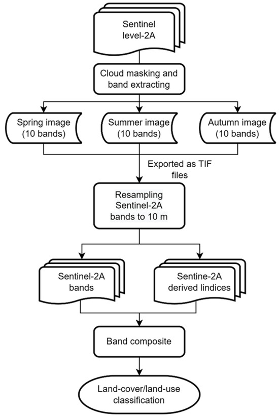
Figure 2.
Flowchart of processing Sentinel-2A images.
Based on the seasonal composited images, three indexes including normalized difference water index (NDWI), soil-adjusted vegetation index (SAVI), and normalized difference vegetation index (NDVI) [56,57,58] were derived for each seasonal composition to facilitate the land cover classification. These indices have been proven to be robust and reliable indicators for discriminating water bodies from vegetation and soil, as well as for tracking changes in vegetation over time [59,60,61,62,63]. As a result, nine index images (three seasonal images × three index images) were generated.
To export the seasonal composited images and their corresponding derived index images, Google Drive was used as an export data receiver. However, due to the size restriction of exportation to Google Drive, the images were exported by dividing each image into three parts of the study area and were stitched again in ENVI 5.6 software (Exelis Visual Information Solutions, Boulder, CO, USA).
Sentinel-2 mission provides multi-spectral (12 bands) at a spatial resolution of 10–60 m. For this study, the 10 m bands (B2, B3, B4, and B8) and 20 m bands (B5, B6, B7, B8, B11, and B12) were used. The bands 1 and 10 were removed as redundant information of coastal aerosol and cirrus-type cloud radiation. To fully utilize the multispectral information provided by the Sentinel-2A satellite, we resampled the bands with a native resolution of 20 m (B5, B6, B7, B8, B11, and B12) down to a finer 10 m resolution in ENVI 5.6 software. The resampled bands were mosaiced with 10 m bands (B2, B3, B4, and B8) to create an image at a resolution of 10 m. Furthermore, the resampled seasonal composition images were ultimately combined with index (NDWI, SAVI, and NDVI) images to form a singular image for land cover/land use classification. Figure 2 shows the flowchart of processing Sentinel-2A images.
Field visits and ancillary datasets were utilized to collect comprehensive landscape information, including land cover/use types and tree species, which facilitated the differentiation of diverse landscapes and improvement of satellite image interpretation. Ground truth data for Sentinel-2A image classification, primarily consisting of homogeneous tree species in the Aizu region, were collected during field visits along major roads and forest trails. A total of 126 sites were visited and the typical land cover and forest types, as well as their GPS locations, were recorded using a MAP64SJZ GPS receiver (Garmin, Olathe, KS, USA) and digitalized. Additionally, the high-quality images and geotagged photos available in Google Earth Pro™ (https://www.google.com/earth/, accessed on 20 March 2021) were used to derive reference information through visual image interpretation. The land cover classes observed were recorded with geo-referenced information, and these records served as an auxiliary reference dataset for selecting regions of interest (ROI). Further supplementary data sources included 10 plots (3 were NLF and 7 were BLF) from the National Forest Inventory (http://www.rinya.maff.go.jp/j/keikaku/tayouseichousa/, accessed on 10 April 2021) for the study area and the forest register of Fukushima Prefecture provided by Forestry Promotion Division of Fukushima, both available in GIS file format. These resources provided crucial tree information (e.g., species, age, and ownership) aiding in tree species identification for satellite image interpretation. Based on our field experience and supplementary data, we selected the sample points (pixels) showing similar features through visual interpretation of images. A total of 23,136 sample points (pixels) of Sentinel-2A images were selected as our ROI. Subsequently, 70% and 30% of these pixels were randomly assigned as training and testing samples following the methodology of Breiman and Spector et al. [64].
Classification categories were defined based on the land use and land cover map products (https://www.eorc.jaxa.jp/ALOS/en/dataset/lulc_e.htm, accessed on 15 March 2021) provided by the Japan Aerospace Exploration Agency (JAXA) and visual interpretation (Table 1).

Table 1.
Land cover and land use classes with descriptions for the Aizu region.
Random forest (RF) classifier was used for image classification. High classification accuracies have been reported for the land cover/use classification of Sentinel-2 data using RF compared with other classifiers such as the maximum likelihood classifier (MLC), support vector machine (SVM), classification tree (CT), and k-nearest neighbor (k-NN) [65,66,67,68]. RF is an ensemble method based on classification and regression trees that can be constructed in parallel without strong dependencies among individual learners [69,70,71]. The decision trees are created based on variables including the object attributes (independent variables) and their visually identified label (dependent variable) of the training set (ROIs) [72]. For each decision tree node, a random subset of the training set is assessed and used to develop other decision trees. By default, two-thirds of the training set (so-called in-bag samples with a total number of 494 samples of all classes) were used for decision tree development, whereas the remaining one-third of the training set (so-called out-of-bag samples with a total number of 277 samples of all classes) were used for assessing the prediction performance of the RF [73]. By aggregating the predictions of all individual decision trees, the final class of a certain land cover type was determined by the prediction with the highest majority vote [72,73,74]. We defined the number of decision trees as 10,000 to build the RF. The classification result was assessed using a confusion matrix [75], the overall classification accuracy, kappa coefficient, producer’s accuracy, and user’s accuracy [76]. Non-forest classes were removed from the resulting classification map so that only forest classes remained.
2.3. Estimation and Mapping of Residual Woody Biomass
2.3.1. Trunk Volume Estimation
As a key parameter in forest ecosystems, trunk volume (TV) (m3/ha) is closely correlated with the aboveground biomass of forest ecosystems and allows for the prediction of all related biomass components (stems, branches, foliage, roots, and understory) for various research purposes.
In this study, we utilized the BGC-ES sub-biomass model developed by Ooba et al. [77] to estimate the TV. The sub-biomass model can estimate the TV based on tree age and tree type information by using the growth function and population function that considers factors like water availability, light, soil nutrients, and forest management. The process began with the estimation of average tree height (hm) as a function of forest age (t), followed by the determination of population number (N), and culminated in the calculation of TV (V).
The average tree height was calculated using a growth function hf (t) as follows:
where hmax is the maximum tree height (m), sc is the site coefficient, and hf (t) is a growth function that is defined by the Mitscherlich [78] (Equation (2)) or Gompertz equations [79] (Equation (3)) as follows:
where hb and hc are species-specific parameters that characterize the growth rate and the shape of the growth curve, respectively.
h = sc hmax hf (t),
hf (t) = 1 − hb exp(−hct),
hf (t) = exp(−hb exp(−hct)),
The population number in a forest unit is estimated using the theoretical 3/2-law [80]. The maximum volume of the trunk of a plant Vmax (m3 ha−1) depends on the maximum population number Nmax (ha−1):
where k and are parameters (Table 2). is an empirical constant typically valued at 1/2. Equation (4) is represented as a line with a slope of −0.5 in a logarithmic coordinated N–V plane.
Table 2.
Parameter values used in equations.
Subsequently, the population number (N) was estimated using the natural mortality curve, which takes into account the intraspecific competition:
where k∗ is a scaling parameter, represents the initial population number (ha−1), and α is an empirical constant typically valued at 1/2, reflecting the 3/2-law of self-thinning.
Finally, trunk volume (V) was calculated by inverting the relationship between volume and population number, integrating the average tree height (hm):
where , , and , were sourced from the National Forestry Agency of Japan [81]. (Table 2), adjusted for the region and tree type. By inputting the age data into these equations, we estimated the TV (V) for individual trees.
To calculate the annual total TV per hectare (Gv, m3 ha−1), TV (V) was multiplied by the population number of trees (ha−1):
Gv = N·V,
It is worth mentioning that the sub-biomass model was developed under relatively simple assumptions (such as an increase in the tree diameter at breast height changes with competition and an increase in the averaged upper-layer tree height mainly depending on the forest age) about the forest ecosystem. Furthermore, the coefficients used for these functions vary with region and tree type. Forest inventory and forest report review are necessary when determining the coefficients. More detailed investigations are necessary for more specific woody biomass estimations.
2.3.2. Trunk Volume Data Preparation
The tree age and tree type information (forest registrator book) of our study area was obtained in GIS file format provided by the Forestry Promotion Division of Fukushima.
As a result of Section 2.3.1, two maps of TV (Gv, m3 ha−1) for NLF and BLF were generated. Then, through the raster calculation in ArcGIS 10.8 software (https://www.esrij.com, accessed on 1 December 2023), the forest map obtained in Section 2.2 was linked geographically with the two TV maps of NLF and BLF by using the information of tree type (NLF or BLF). Thus, an integrated TV (Gv, m3 ha−1) map of 10 m resolution was created.
A flowchart summarizing the preparation of the TV map is shown in Figure 3 (yellow color background).
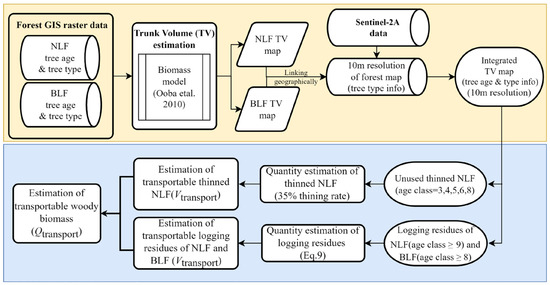
Figure 3.
The flowchart of 10 m resolution of the TV and potential residual woody biomass estimation for the Aizu region. NLF stands for needle-leaf forest and BLF stands for broad-leaf forest. Details of estimation of transportable woody biomass (blue background) are described in Section 2.3.3.
2.3.3. Estimation of Forest Residual Biomass
Forest residual biomass (waste woody biomass) is comprised of residues resulting from two kinds of anthropogenic practices (thinning and logging). Estimations of forest residual biomass were performed separately for the two different practices (thinning and logging) (Figure 3).
Thinning activity, according to the local forestry management plan [53], was performed mainly on certain ages of young needle-leaf trees to improve the health and growth of a forest. Therefore, the estimation of thinned residual biomass was focused on NLF of age classes 3–6 and 8 (one age class is equal to 5 years). BLF was excluded from this step, as there were no thinning plans for BLF. The thinning rate was 35% for trees of all thinning ages combined [53]. The entire portion of each thinned NLF was assumed to be used for bioelectricity generation. The available thinned NLF volume was calculated by multiplying the annual total NLF TV (Gv m3 ha−1) by a thinning rate of 35%.
For logging activity, according to the local forestry management plan [53], cutting ages for logging were performed mainly on NLF trees aged at least 45 years (age class 9 or greater) and BLF trees aged at least 40 years (age class 8 or greater). Unlike in the case of thinning, the logging residue including branches, leaves, stumps, roots, tops, and bark that had been stripped from the harvested raw wood and was assumed to be used for bioenergy generation. In the Aizu region, logging residues are typically found at felling sites in the forest or wood piles alongside the road [53].
The amount of forest logging residue was estimated by using the method developed by Japan’s Forestry and Forest Products Research Institute (Equation (8)):
where
Qresidue represents the quantity of dry wood logging residue (t ha−1);
Gv represents the annual logging of trunk volume per unit (m3 ha−1);
fresidue represents the logging residue generation coefficient (0.07 for NLF and 0.091 for BLF) [82];
Wd represents the 15% air-dry water content of logged woods.
Because the utilization of potential woody biomass is largely restricted by transportation infrastructures for the collection of woody biomasses and its transportation out of the forest, we needed to consider the road network (density of the forest road and the distance from the road required for wood collection) in forests. Therefore, the quantities of transportable (available for energy production) thinned woods and logging residues in each pixel in the raster data were further estimated by integrating the road network information, including the density of the forest road network and the distance from the road at which point wood is collectible using Equation (9). It is worth mentioning that this method has been commonly used in Japan and is interpretable across multiple disciplines and by policymakers [14,33,82]. However, the use of a fixed road density across the study area may not accurately capture the variations in road network densities, potentially leading to overestimations or underestimations of transportable biomass in different sub-regions such as remote mountainous areas (with less road density) and lower areas (with higher road density).
where
Vtransport represents the annual volume of transportable residual woody biomass (m3);
GV thinned/residual represents the annual volume of thinned NLF or logging residues of NLF or BLF (m3 ha−1);
Droad represents the density of the forest road network (6.29 m/ha);
Rcollect represents the collection distance for forest residues, which is assumed to be 25 m from the forest road to the mountain slope and 25 m to the valley slope, equalling a total of 50 m from the roads [83];
10−4 is the scale factor (ha m−2).
The mass of the transportable (available for bioenergy production) forest residual biomass (Qtransport) in tonnes of dry matter per hectare per year (t dry-weight (ha−1) in each pixel was derived from the following formula:
where
Dbulk represents the bulk density of NLF (0.314 t m−3) or BLF (0.573 t m−3) [84].
A flowchart summarizing the process of the overall estimation is shown in Figure 2 (blue color background).
2.3.4. Available Bioelectricity Potential
The available potential of woody bioelectricity represents the available quantity of biomass that can be technically and economically harvested and used for energy purposes [85]. In Japan, wood fuels used for electricity generation are generally made from residuals from the sawmill process, the manufacture of wood products and construction, and harvesting/thinning residuals in the forest. The available bioelectricity potential from combustion was evaluated using Equation (11), developed by Tatebayashi et al. [86].
where
Ebiosolid represents the woody biomass energy (Gigajoule ha−1, hereafter referred to as GJ ha−1);
Qtransport represents the dry wood matter of transportable biomass (t ha−1);
Wp represents the water content percentage, which was set at 10% for air-dried processed wood residues, and (1 − Wp)−1 represents the composition ratio of wood solids;
YR represents the yield (the ratio of the output to the total input of materials in a process), and 20% was set as the output loss of wood materials during the processing;
LHV represents the lower heating value of 16 GJ t−1.
To make the unit of TV map pixel (10 × 10 m2) consistent with the units of the quantity of transportable (collectible) residual biomass and the residual biomass energy (Qtransport and Ebiosolid, respectively), we converted the units of Qtransport and Ebiosolid from t ha−1 and GJ ha−1 to t 100 m−2 and GJ·100 m−2 by multiplying them by a scale factor of 0.01. Each pixel then represented the biomass quantity/volume of a certain type of tree.
At last, the overall quantity of residual biomass over the study area was calculated by multiplying the biomass quantity/volume values with the statistically counted pixel numbers that share the same type of tree and age. Thus, the overall quantity of transportable woody biomass and the energy feedstock potential of the whole study area was obtained.
However, the amount of woody biomass that can be collected and used for power generation is restricted by various factors such as terrain features, the road network for collecting and transporting wood materials, and the collection range from the power plant to the chip processing sites. We selected the Green Power Aizu Power Plant as the target of this analysis as it is the first local woody biomass power plant and is supported by MAFF, aiming to recycle local waste woody biomass into electricity generation. The sources of fuelwood are thinned and logging residues. The electricity generated mainly serves the Aizu region’s largest city of Wakamatsu, catering to power producers and suppliers of industrial electricity. The plant’s electricity generation capacity (generating-end output) is about 5700 kW, and the total annual electricity generation capacity is 167,443.2 GJ. Operating 24 h a day for 340 days a year, the plant requires an annual feedstock of 36,000 t of dried chips.
Therefore, to more accurately estimate the realistic potential of accessible woody biomass for the power plant, we used data from the forest plan of the Aizu Region [53] to set and apply several filters to the local forest register data. The filters and the reasons for their application were as follows:
- (1)
- Because the national average woody material collection radius is 50 km [87], which is also the operating radius of the towable wood chippers that are adopted by most of the small scale power plants, the area within 50 km was set as the maximum biomass-collection buffer radius to the Green Energy Aizu Power Plant.
- (2)
- Under the distance reachable by lumber-collecting machinery, the distance from the center of each unit of each forest land unit (forest compartment) to the nearest road was set at no more than 500 m.
- (3)
- The slope of land was set at no more than 35° due to difficulties in logging/thinning, collecting, and transporting operations. Moreover, many areas with slopes greater than 35° are classified as protected land to prevent natural disasters such as landslides and soil erosion.
- (4)
- Forests in which cutting was forbidden were not included, as local government has strict land-use rules to protect national parks or lands that are at a high risk of natural disasters.
Based on the estimated bioelectricity potential within a 50 km radius of the power plant, we estimated the potential reduction in CO2 emissions by replacing coal-fired power generation with biomass-fired power generation. This estimation was derived from the difference in CO2 emissions between the biomass-fired generation system (0.0618 tons CO2/MWh) and the coal-fired generation system (0.96 tons CO2/MWh) in Japan [88].
3. Results
3.1. Forest Cover Mapping
A total of 84% of the study area was classified as forest (Figure 4). Almost 32% of the forest was BLF, distributed below an elevation of 1400 m across the study area. Most of these BLFs are secondary woods planted after clean cutting for woodfires and mainly distributed around villages. A total of 52% of the forest was NLF, most of which had been planted along streams, rivers, urban areas, and villages below 1000 m elevation.
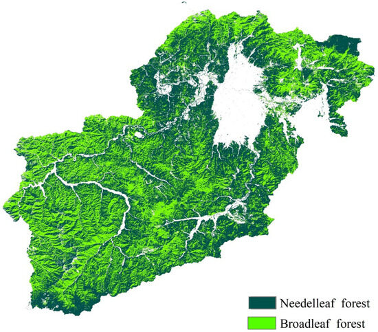
Figure 4.
Forest cover map of the Aizu region. The blank areas are other non-forest land types including rivers, roads, built-up areas, and cropland.
Table 3 gives an accuracy assessment of land cover classification results. The class-specific producer’s accuracies were 97.93% and 92.57% for NLF and BLF, respectively. An overall accuracy of 92.32% and a Kappa index of 0.9086 indicate a satisfactory accuracy, which underscores the robustness of the RF classifier in incorporating the multi-temporal dimension of the dataset into the analysis and evaluating the different features which are critical for accurate classification. In previous research, multitemporal data and RF classification showed satisfying forest mapping and facilitated further above-ground biomass estimation [89,90,91,92].
Table 3.
Accuracy of forest classification for the Aizu region.
However, class confusion between NLF and BLF did occur. Some tree species have different patterns of phenological variation in their leaves and flowering over seasons (e.g., BLF leaves do not always turn yellow or red in autumn, and the leaves of certain pine tree species (such as Metasequoia) turn reddish in autumn and winter). This could have caused confusion between NLF and BLF, as the spectral reflection of plants was one of the indicators used in our classification. Some of the pixels of Sentinel-2A contained mixed forest stands (e.g., broad-leaf and needle-leaf, or mixed-age) and were classified into homogeneous forest types (NLF/BLF). Furthermore, due to the limited data set that contained forest information about our study area, we only used two general forest types (NLF and BLF) for the biomass estimation. As the biomass varies among different tree species, there might be some discrepancies between our estimation with the actual forest biomass. Combining active remote sensing data such as LiDAR/SAR that can be used to extract forest structural attributes including tree height and classifying tree species can enhance the precision of detailed forest mapping and biomass estimation.
3.2. Spatial Analysis of Forest Residual Biomass
3.2.1. Analysis of Thinned Residue Biomass
For thinned residue biomass, we mapped the spatial distribution of transportable thinned residue biomass (Figure 5a) and bioelectricity potential (Figure 5b).
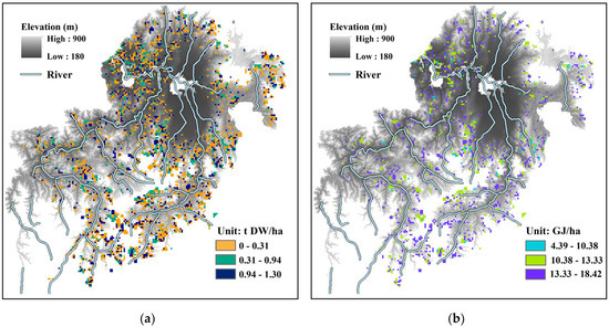
Figure 5.
Spatial distribution of (a) Transportable quantity of biomass of thinned NLF (t dry-weight ha−1); (b) Bioelectricity potential of thinned NLF based on transportable biomass (GJ ha−1). DW stands for dry-weight. NLF stands for needle-leaf forest and BLF stands for broad-leaf forest.
There was a uniform distribution pattern of both low and high biomass quantity across the study area. According to elevation information provided by the forest register, the residue biomass left by thinning was distributed mainly at elevations of 180 m to 900 m along the rivers over the study area, except in populated areas such as Wakamatsu city.
The TV (Gv in table) of NLF (ages 15, 20, 25, 30, and 40) ranged from 89.34 to 374.54 m3 ha−1 year−1. The volume of residues (Gv-residue) extracted from thinned NLF trees ranged from 31.27 to 131.09 m3 ha−1 year−1. The corresponding mass of residues (Qresidue) ranged from 9.82 to 41.46 t dry-weight ha−1 year−1 with a mean value of 24.08 t dry-weight ha−1 year−1. Of this residue mass, the transportable amount of residues (Qtransport) varied from 0.31 to 1.29 t dry-weight ha−1 year−1, available for delivery to a power plant for energy production. Consequently, the bioelectricity potential (Ebiosolid) of this transportable mass of residues ranged from 4.1 to 18.10 GJ ha−1 with a mean value of 10.77 GJ ha−1 (Table 3).
3.2.2. Analysis of Logging Residue Biomass
The distributions of logging residue biomass and corresponding bioelectricity production potential of NLF (Figure 6a,b) and BLF (Figure 6c,d) were mapped separately.
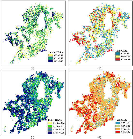
Figure 6.
Spatial distributions of (a) Transportable quantity of biomass of NLF logging residues (t dry-weight ha−1); (b) Bioelectricity potential of NLF logging residues based on transportable biomass (GJ ha−1); (c) Transportable quantity of biomass of BLF logging residues (t dry-weight ha−1); (d) Bioelectricity potential of BLF logging residues based on transportable biomass (GJ ha−1). NLF stands for needle-leaf forest, and BLF stands for broad-leaf forest.
As in the case of thinning residues, the logging residues also showed a general uniform distribution pattern over the study area. However, some high biomass values (dark blue in Figure 6a) were distributed in the south-western part of our study area, which is a remote mountainous area with relatively higher elevation than other parts of the study area and has less residential area.
The TV of NLF (aged at least 45 years) ranged from 89.34 to 374.54 m3 ha−1 year−1. The logging residue mass ranged from 9.17 to 14.26 t dry-weight ha−1 with a mean value of 12.79 t ha−1, while the mean value of mass available for energy production (transportable amount) reduced to 0.29–0.45 t dry-weight ha−1 with a mean value of 0.4 t ha−1. The corresponding bioelectricity potential ranged from 4.1 to 6.38 GJ ha−1 with a mean value of 5.72 GJ ha−1 (Figure 7).The TV of BLF (aged at least 40 years) did not vary markedly (range, 128.5 to 138.58 t dry-weight ha−1) because the growing volume tends to be stable for mature BLF. Compared with NLF, their mean values of logging residues were close, but the minimum value of BLF was greater than NLF while the maximum value of BLF was smaller than NLF. The corresponding bioelectricity potential ranged from 3 to 3.23 GJ—which is lower than NLF (Figure 7).
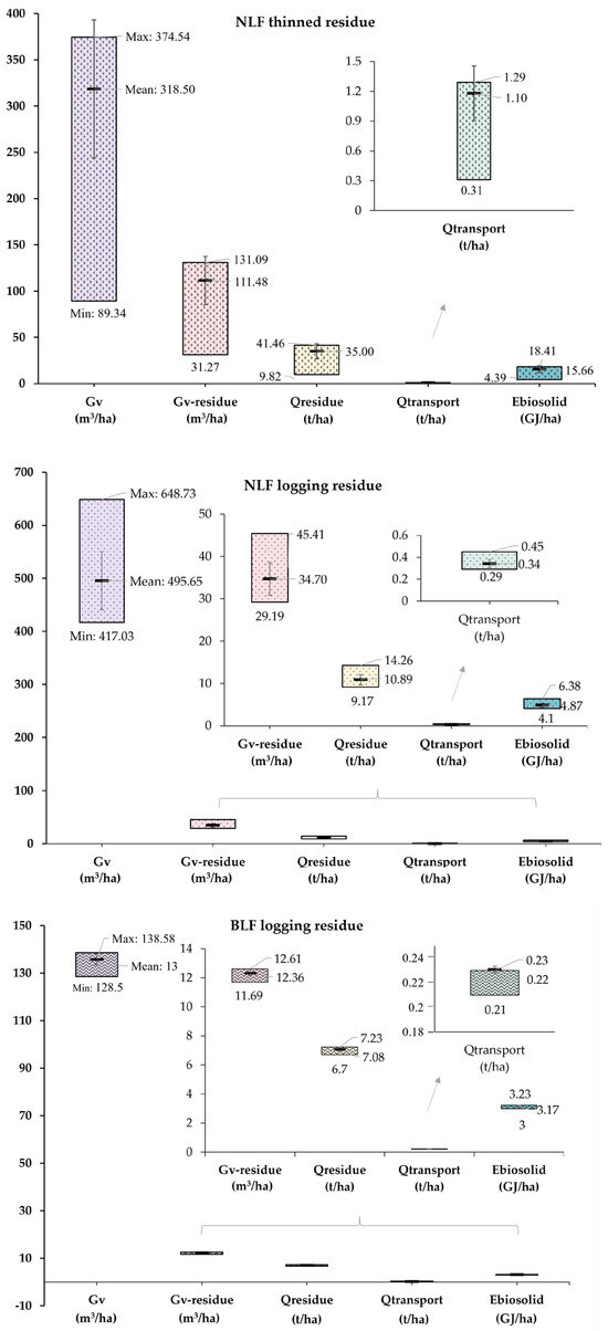
Figure 7.
Values of parameters of thinning and logging activities in needle-leaf and broad-leaf forests. Gv refers to trunk volume, Gv-residue refers to thinned residue volume, Qresidue refers to thinned residue mass, Qtransport refers to thinned residue mass available for energy production, and Ebiosolid refers to bioelectricity production potential. NLF stands for needle-leaf forest, BLF stands for broad-leaf forest. Lines inside the boxes represent error bars.
3.2.3. Estimation of Potential Bioelectricity
By using the pixel-based values of estimated bioelectricity for different tree age classes of the residues of thinned NLF and the logging residues of BLF and NLF, we calculated the total amount of potential bioelectricity for each tree age class by multiplying the pixel values of bioelectricity by the number of pixels that shared the same values. The sum value of the calculated total potential bioelectricity was then regarded as the overall potential bioelectricity of the entire study area. All the transportable amounts of forest residues can provide 744,964 tons of woody biomass. The relative potential bioelectricity of 2018 was approximately 2,717,366 GJ (627,046 GJ for thinned NLF, 1,031,436 GJ for BLF logging residues, and 1,058,884 GJ for NLF logging residues), which is 16.2 times the plant’s power-generating capacity. NLF logging residues contributed to 39% of the Aizu region’s total bioelectricity potential, BLF logging residues contributed to 38%, and thinned NLF contributed to 23%. According to the Wood Demand Chart of 2020 [16], the coefficients for converting wood to chips are 2.2 for NLF and 1.7 for BLF. After conversion of the collectable dry-matter biomass quantity to chip production, the total dried-chip production potential was approximately 246,052 t (63,823 t for thinned NLF; 74,451 t for BLF logging residues; and 107,778 t for NLF logging residues). The potential chip production is more than 6.8 times the annual chip demand of the Green Energy Aizu Power Plant which requires an annual feedstock of 36,000 t of dried chips.
Within the extracted 50 km radius of the Green Energy Aizu Power Plant, approximately 70% of the extracted forest was NLF and 30% was BLF. The forest residues within the extracted area can provide 45,925 tons of woody biomass. The total dried-chip production potential was approximately 22,960 t, which can meet the 64% of the annual chip demand of the power plant. The spatial distribution of potential chip production indicated the values range from 0.0005 to 0.645 t/ha with a majority of 0.233–0.645 t/ha (Figure 8a). The estimated total energy potential was 261,507 GJ—approximately 1.6 times the annual electricity-generation capacity of the power plant. The spatial distribution of potential bioelectricity indicated that most forests within the area have the potential to provide 3.2–6.3 GJ/ha of bioelectricity (as represented by the blue color in Figure 8b). The potential bioelectricity would also supply 2% of the total population-based energy consumption of Wakamatsu city in 2015 (102.43 GJ/person for a population of 124,100 people) [93,94]. Additionally, the substitution of coal fuel with this residual biomass is estimated to reduce CO2 emissions by approximately 65,246 tons/year. The reduction of CO2 emissions from the entire study area’s residual biomass-fired power generation was estimated to be 677,983 tons/year, which corresponds to 1.84% of the Fukushima Prefecture’s CO2 emissions as of 2019 (36,876,452 tons/year) [95].
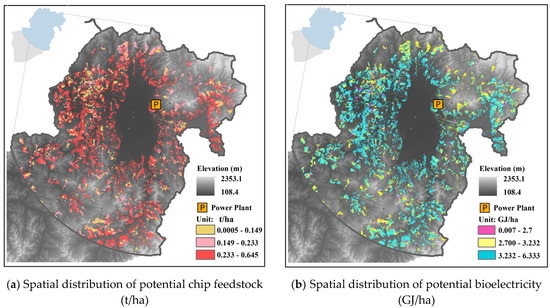
Figure 8.
Distribution map of (a) Potential bioelectricity and (b) Potential chip feedstock of the extracted forest area within 50 km of the Green Energy Aizu Power Plant for the Aizu region.
4. Discussion
This study used growth and population functions from a sub-biomass model of BGC-ES developed by Ooba [29]. BGC-ES is advantageous for estimating forest resource dynamics as it incorporates factors such as water, light, soil nutrients, and forest management into the simulation. It also facilitates area-wide estimations easily, particularly when using satellite imagery-based land cover classifications as the data source. However, since it provides estimations of average size and growth of trees, more detailed investigations are necessary for more specific woody biomass projects. In the present study, it was observed that although NLF for thinning has a lower TV (mean value: 219.1 m3 ha−1) compared to NLF for logging (mean values: 581.99 m3 ha−1) due to the younger age of the thinned trees, it yields more residues per unit (mean value: 76.68 m3 ha−1), as the whole tree was cut down and considered as a biomass resource in thinning activities (Figure 9). In logging activities, only the stripped parts of the tree, excluding the merchantable trunk, are considered as residual biomass. Among the logging residues, the BLF has a lower TV and fewer residues compared to NLF. This is because most of the trees in BLF areas are mature, and their trunk volumes are relatively stable. NLF and BLF logging residues together account for 77% of the total residual biomass in the study area (Figure 9), indicating that they are the primary contributors to the bioenergy production potential.
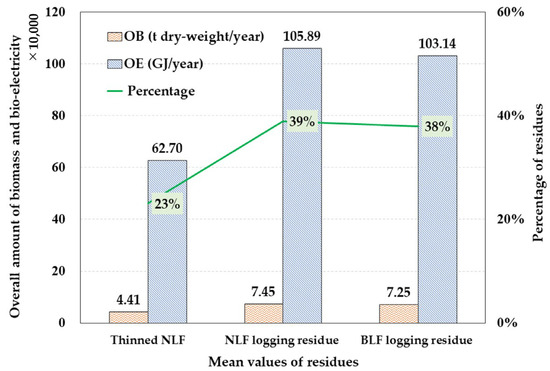
Figure 9.
Overall amount of residual biomass and potential energy for bioelectricity.
In the present study, the estimations for transportable biomass were based on the existing forest road network and ground slope. As a result, the calculated values for both biomass and bioelectricity potential were significantly lower than potential utilization of the abundant forest resources in the study area. One limitation of our study is the adoption of a fixed road density and thinning/logging intensity to represent the entire study area, which may not capture the variations in road network densities in individual sub-compartments of forest. Estimating availability based on road density in each sub-compartment would yield a more accurate biomass availability estimation and facilitate the investigation of optimized strategies adapted to different availabilities and logistics.
According to Yoshioka et al. [22], the lowest costs for hauling, transporting, and chipping residues range from USD 150/t to USD 227/t of dry biomass. Consequently, the total cost for transporting residual biomass in our study area was calculated to range from USD 28,659,750 to USD 43,371,755. Compared to processing residues alongside forest roads or at plants, processing them directly at thinning/logging sites using advanced machinery is preferable for cost minimization. This is particularly challenging given the current state of the Japanese forestry industry, which suffers from low-capacity forestry machines and a lack of well-trained operators [96]. The shortage of well-trained operators is a multifaceted issue, driven by an aging workforce, insufficient training and education, and the slow adoption of technology in the forestry industry [24]. To achieve more efficient harvesting, processing, and management of forest resources, thereby minimizing procurement costs and increasing overall productivity, it is essential to have better machines and well-trained operators skilled in the use of advanced forestry equipment and implementing sustainable forest management practices [22,97]. Government initiatives that provide skill-building opportunities in forestry and revitalizing the forestry workforce is necessary [5]. Furthermore, subsidies aimed at expanding current road density in woodland areas and supporting the development of efficient forestry techniques are crucial for improving this situation. Such measures would attract more forestry businesses and facilitate the conversion of forest waste into energy.
Additionally, power generation based on residual biomass has the potential to reduce CO2 emissions by replacing coal-fired power generation. To promote renewable energy use and reduce CO2 emissions, Japan has implemented policies and measures such as the feed-in tariff (FIT) system and a carbon tax. However, the level of carbon tax in Japan is lower than in many other countries. Therefore, the introduction of more robust measures such as large-scale carbon pricing and emissions trading systems, is essential to further incentivize the shift towards renewable energy sources and achieve more substantial reductions in CO2 emissions.
Removing waste residual biomass has potential ecological impacts on soil nutrients, biodiversity, and carbon cycling. Its removal could lead to soil nutrient depletion, reduced habitat complexity, and altered forest dynamics [98]. Careful management is essential to balance biomass removal with ecological sustainability.
5. Conclusions
The availability and potential of forest biomass and its energy utilization from logging residues and thinned trees were discussed with the combination of BGC-ES sub-biomass model, remote sensing, and GIS tools. Firstly, a distribution map of forest biomass map was completed by combing Sentinel-2A-derived forest maps and tree trunk volume modeling. Then, the transportable availability of residual biomass was estimated taking into consideration thinning/logging intensities, road density, and wood collectable range. Finally, the corresponding bioelectricity generation potential and its CO2 reduction effects was discussed.
As a result, NLF logging residue (the annual available amount was 74,453 t/y (dry weight)) proved to be the primary biomass contributor to the bioelectricity potential (2,717,366 GJ), followed by broad-leaved forests (72,523 t/y (dry weight)) and thinned trees (44,089 t/y (dry weight)). The forests located within a 50 km radius of this power plant can supply biomass (45,925 t/y (dry weight)) that equates to 1.6 times the facility’s capacity, also fulfilling 2% of the energy demands of the region’s central city. By substituting a coal-fired power generation system with a biomass-fired system, a reduction of CO2 emissions of 677,983 tons/year can be achieved from the study area’s residual biomass, which can potentially be contributed to a reduction of 1.84% of the Fukushima Prefecture’s yearly CO2 emissions. The results highlight the bioelectricity potential and carbon-neutral capacity of residual biomass. This encourages government initiatives and policy inclinations to sustainably boost the production of bioenergy derived from residual biomass.
A significant challenge in harnessing this potential is the existing forest road network as well as forestry machinery, which poses constraints on the forwarding and transportation of usable residual wood biomass. This underscores the critical need to enhance the forest road infrastructure and calls for both technical and financial support for the forestry sector. Future studies could apply economic feasibility analyses to assess the collection and transportation of residual forest biomass for supplying sustainable and low-carbon bioenergy feedstocks.
Author Contributions
Conceptualization, T.Q., M.O. and M.F.; methodology, T.Q. and M.O.; software, T.Q.; validation, T.Q. and S.N.; formal analysis, T.Q., T.M., C.H. and A.N.; investigation, T.Q.; resources, M.O., T.M., C.H. and A.N.; writing—original draft preparation, T.Q.; writing—review and editing, M.O., S.N. and M.F.; visualization, T.Q.; supervision, M.F.; funding acquisition, M.F. All authors have read and agreed to the published version of the manuscript.
Funding
This work was funded by the Environment Research and Technology Development Fund (JPMEERF20223C02) of Environmental Restoration and Conservation Agency of Japan.
Data Availability Statement
Data are available upon request.
Acknowledgments
The authors are grateful to Saritha Sudharmma Vishwanathan, Yanyan Yu, and Ziyan He for their helpful suggestions regarding the manuscript. The authors thank Watanabe for her assistance in obtaining data and contribution to the analysis.
Conflicts of Interest
The authors declare no conflicts of interest.
References
- United Nations Development Programme. Access to Energy and Human Development. 2008. Available online: https://hdr.undp.org/system/files/documents/gayeamiepdf.pdf (accessed on 20 January 2022).
- Harvey, F. ‘Carbon bubbble’ poses serious threat to UK economy, MPs warn. The Guardian, 6 March 2014. [Google Scholar]
- Mercure, J.-F.; Pollitt, H.; Viñuales, J.E.; Edwards, N.R.; Holden, P.B.; Chewpreecha, U.; Salas, P.; Sognnaes, I.; Lam, A.; Knobloch, F. Macroeconomic impact of stranded fossil fuel assets. Nat. Clim. Change 2018, 8, 588–593. [Google Scholar] [CrossRef]
- Wuebbles, D.J.; Jain, A.K. Concerns about climate change and the role of fossil fuel use. Fuel Process. Technol. 2001, 71, 99–119. [Google Scholar] [CrossRef]
- Goh, C.S.; Aikawa, T.; Ahl, A.; Ito, K.; Kayo, C.; Kikuchi, Y.; Takahashi, Y.; Furubayashi, T.; Nakata, T.; Kanematsu, Y.; et al. Rethinking sustainable bioenergy development in Japan: Decentralised system supported by local forestry biomass. Sustain. Sci. 2020, 15, 1461–1471. [Google Scholar] [CrossRef]
- Baker, J.S.; Crouch, A.; Cai, Y.; Latta, G.; Ohrel, S.; Jones, J.; Latané, A. Logging residue supply and costs for electricity generation: Potential variability and policy considerations. Energy Policy 2018, 116, 397–409. [Google Scholar] [CrossRef] [PubMed]
- Matsuoka, Y.; Shirasawa, H.; Hayashi, U.; Aruga, K. Annual Availability of Forest Biomass Resources for Woody Biomass Power Generation Plants from Subcompartments and Aggregated Forests in Tohoku Region of Japan. Forests 2021, 12, 71. [Google Scholar] [CrossRef]
- Brown, M.A.; Favero, A.; Thomas, V.M.; Banboukian, A. The economic and environmental performance of biomass as an “intermediate” resource for power production. Util. Policy 2019, 58, 52–62. [Google Scholar] [CrossRef]
- Li, M.; Lenzen, M.; Yousefzadeh, M.; Ximenes, F.A. The roles of biomass and CSP in a 100% renewable electricity supply in Australia. Biomass Bioenergy 2020, 143, 105802. [Google Scholar] [CrossRef]
- International Energy Agency (IEA). Japan 2021—Energy Policy Review. 2021. Available online: www.iea.org/t&c/ (accessed on 12 July 2022).
- International Energy Agency (IEA). “World Balance Documentation,” Paris, France. 2021. Available online: https://iea.blob.core.windows.net/assets/20a89a1b-634c-41f1-87d1-d218f07769fb/WORLDBAL_Documentation.pdf (accessed on 14 July 2022).
- Agency for Natural Resources and Energy. Inefficient Coal Phasing out and Renewable Dominated Power Generation. 2020. Available online: https://www.meti.go.jp/shingikai/enecho/denryoku_gas/denryoku_gas/pdf/026_03_00.pdf (accessed on 15 July 2022).
- Ministry of Economy, Trade and Industry (METI). Japan’s 2050 Carbon Neutral Goal. 2020. Available online: https://www.meti.go.jp/english/policy/energy_environment/global_warming/roadmap/index.html (accessed on 5 April 2022).
- Ministry of Agriculture, Forestry and Fishery (MAFF). Annual Report on Forest Forestry in Japan FY 2018. 2018. Available online: https://www.rinya.maff.go.jp/j/kikaku/hakusyo/30hakusyo_h/all/index.html (accessed on 15 July 2022).
- Yoshioka, T.; Sakurai, R.; Aruga, K.; Sakai, H.; Kobayashi, H.; Inoue, K. A GIS-based analysis on the relationship between the annual available amount and the procurement cost of forest biomass in a mountainous region in Japan. Biomass Bioenergy 2011, 35, 4530–4537. [Google Scholar] [CrossRef]
- Ministry of Agriculture, Forestry and Fishery (MAFF). Wood Demand Chart of 2020. 2021. Available online: https://www.maff.go.jp/j/tokei/kouhyou/mokuzai_zyukyu/index.html (accessed on 20 July 2022).
- Ooba, M.; Hayashi, K.; Fujii, M.; Fujita, T.; Machimura, T.; Matsui, T. A long-term assessment of ecological-economic sustainability of woody biomass production in Japan. J. Clean. Prod. 2015, 88, 318–325. [Google Scholar] [CrossRef]
- Ahl, A.; Eklund, J.; Lundqvist, P.; Yarime, M. Balancing formal and informal success factors perceived by supply chain stakeholders: A study of woody biomass energy systems in Japan. J. Clean. Prod. 2018, 175, 50–59. [Google Scholar] [CrossRef]
- Hondo, H.; Moriizumi, Y. Employment creation potential of renewable power generation technologies: A life cycle approach. Renew. Sustain. Energy Rev. 2017, 79, 128–136. [Google Scholar] [CrossRef]
- Kinoshita, T.; Inoue, K.; Iwao, K.; Kagemoto, H.; Yamagata, Y. A spatial evaluation of forest biomass usage using GIS. Appl. Energy 2009, 86, 1–8. [Google Scholar] [CrossRef]
- Nagatomo, Y.; Ozawa, A.; Kudoh, Y.; Hondo, H. Impacts of employment in power generation on renewable-based energy systems in Japan—Analysis using an energy system model. Energy 2021, 226, 120350. [Google Scholar] [CrossRef]
- Yoshioka, T.; Aruga, K.; Nitami, T.; Sakai, H.; Kobayashi, H. A case study on the costs and the fuel consumption of harvesting, transporting, and chipping chains for logging residues in Japan. Biomass Bioenergy 2006, 30, 342–348. [Google Scholar] [CrossRef]
- Ohta, H. The Analysis of Japan’s Energy and Climate Policy from the Aspect of Anticipatory Governance. Energies 2020, 13, 5153. [Google Scholar] [CrossRef]
- Forestry Agency. State of Japan’s Forests and Forest Management. 2019. Available online: https://www.maff.go.jp/e/policies/forestry/attach/pdf/index-8.pdf (accessed on 25 July 2022).
- Yoshioka, T.; Aruga, K.; Nitami, T.; Kobayashi, H.; Sakai, H. Energy and carbon dioxide (CO2) balance of logging residues as alternative energy resources: System analysis based on the method of a life cycle inventory (LCI) analysis. J. For. Res. 2005, 10, 125–134. [Google Scholar] [CrossRef]
- Zanchi, G.; Pena, N.; Bird, N. Is woody bioenergy carbon neutral? A comparative assessment of emissions from consumption of woody bioenergy and fossil fuel. GCB Bioenergy 2012, 4, 761–772. [Google Scholar] [CrossRef]
- Fujioka, Y. Annual Report on Forest and Forestry in Japan, Fiscal Year 2014 (Notes) (Review of Government Report). For. Econ. 2015, 68, 29–34. [Google Scholar] [CrossRef]
- Jackson, S.L. Dusty roads and disconnections: Perceptions of dust from unpaved mining roads in Mongolia’s South Gobi province. Geoforum 2015, 66, 94–105. [Google Scholar] [CrossRef]
- Ooba, M.; Fujita, T.; Mizuochi, M.; Fujii, M.; Machimura, T.; Matsui, T. Sustainable Use of Regional Wood Biomass in Kushida River Basin, Japan. Waste Biomass Valoriz. 2012, 3, 425–433. [Google Scholar] [CrossRef]
- Battuvshin, B.; Matsuoka, Y.; Shirasawa, H.; Toyama, K.; Hayashi, U.; Aruga, K. Supply potential and annual availability of timber and forest biomass resources for energy considering inter-prefectural trade in Japan. Land Use Policy 2020, 97, 104780. [Google Scholar] [CrossRef]
- Yamaguchi, R.; Aruga, K.; Nagasaki, M. Estimating the annual supply potential and availability of timber and logging residue using forest management records of the Tochigi prefecture, Japan. J. For. Res. 2014, 19, 22–33. [Google Scholar] [CrossRef]
- Yanagida, T.; Yoshida, T.; Kuboyama, H.; Jinkawa, M. Relationship between Feedstock Price and Break-Even Point of Woody Biomass Power Generation under FIT Program. J. Jpn. Inst. Energy 2015, 94, 311–320. [Google Scholar] [CrossRef]
- New Energy and Industrial Technology Development Organization (NEDO). GIS Database of the Estimation of Biomass Potential and Effective Usable Capacity. 2011. Available online: http://app1.infoc.nedo.go.jp/biomass/ (accessed on 11 January 2020).
- Grabska, E.; Hostert, P.; Pflugmacher, D.; Ostapowicz, K. Forest Stand Species Mapping Using the Sentinel-2 Time Series. Remote Sens. 2019, 11, 1197. [Google Scholar] [CrossRef]
- Lister, A.J.; Andersen, H.; Frescino, T.; Gatziolis, D.; Healey, S.; Heath, L.S.; Liknes, G.C.; McRoberts, R.; Moisen, G.G.; Nelson, M.; et al. Use of Remote Sensing Data to Improve the Efficiency of National Forest Inventories: A Case Study from the United States National Forest Inventory. Forests 2020, 11, 1364. [Google Scholar] [CrossRef]
- Shifley, S.R.; He, H.S.; Lischke, H.; Wang, W.J.; Jin, W.; Gustafson, E.J.; Thompson, J.R.; Thompson, F.R.; Dijak, W.D.; Yang, J. The past and future of modeling forest dynamics: From growth and yield curves to forest landscape models. Landsc. Ecol. 2017, 32, 1307–1325. [Google Scholar] [CrossRef]
- European Space Agency (ESA). Sentinel-2 Missions-Sentinel Online; European Space Agency (ESA): Paris, France, 2014. Available online: https://sentinels.copernicus.eu/web/sentinel/missions/sentinel-2 (accessed on 9 February 2020).
- Malenovský, Z.; Rott, H.; Cihlar, J.; Schaepman, M.E.; García-Santos, G.; Fernandes, R.; Berger, M. Sentinels for science: Potential of Sentinel-1, -2, and -3 missions for scientific observations of ocean, cryosphere, and land. Remote Sens. Environ. 2012, 120, 91–101. [Google Scholar] [CrossRef]
- Belgiu, M.; Csillik, O. Sentinel-2 cropland mapping using pixel-based and object-based time-weighted dynamic time warping analysis. Remote Sens. Environ. 2018, 204, 509–523. [Google Scholar] [CrossRef]
- Kindu, M.; Schneider, T.; Teketay, D.; Knoke, T. Land Use/Land Cover Change Analysis Using Object-Based Classification Approach in Munessa-Shashemene Landscape of the Ethiopian Highlands. Remote Sens. 2013, 5, 2411–2435. [Google Scholar] [CrossRef]
- Nelson, M. Evaluating Multitemporal Sentinel-2 Data for Forest Mapping Using Random Forest. Available online: http://www.diva-portal.org/smash/get/diva2:1138282/FULLTEXT01.pdf (accessed on 4 September 2019).
- Franklin, J.; Hiernaux, P.H.Y. Estimating foliage and woody biomass in Sahelian and Sudanian woodlands using a remote sensing model. Int. J. Remote Sens. 1991, 12, 1387–1404. [Google Scholar] [CrossRef]
- Steininger, M.K. Satellite estimation of tropical secondary forest above-ground biomass: Data from Brazil and Bolivia. Int. J. Remote Sens. 2000, 21, 1139–1157. [Google Scholar] [CrossRef]
- Dai, S.; Zheng, X.; Gao, L.; Xu, C.; Zuo, S.; Chen, Q.; Wei, X.; Ren, Y. Improving maps of forest aboveground biomass: A combined approach using machine learning with a spatial statistical model. Biogeosci. Discuss. 2020, 1–35, preprint. [Google Scholar] [CrossRef]
- Zheng, D.; Rademacher, J.; Chen, J.; Crow, T.; Bresee, M.; Le Moine, J.; Ryu, S.-R. Estimating aboveground biomass using Landsat 7 ETM+ data across a managed landscape in northern Wisconsin, USA. Remote Sens. Environ. 2004, 93, 402–411. [Google Scholar] [CrossRef]
- Lu, D. The potential and challenge of remote sensing-based biomass estimation. Int. J. Remote Sens. 2006, 27, 1297–1328. [Google Scholar] [CrossRef]
- Lu, D.; Chen, Q.; Wang, G.; Liu, L.; Li, G.; Moran, E. A survey of remote sensing-based aboveground biomass estimation methods in forest ecosystems. Int. J. Digit. Earth 2014, 9, 63–105. [Google Scholar] [CrossRef]
- Brown, S.; Gaston, G. Use of forest inventories and geographic information systems to estimate biomass density of tropical forests: Application to tropical Africa. Environ. Monit. Assess. 1995, 38, 157–168. [Google Scholar] [CrossRef]
- Drusch, M.; Del Bello, U.; Carlier, S.; Colin, O.; Fernandez, V.; Gascon, F.; Hoersch, B.; Isola, C.; Laberinti, P.; Martimort, P.; et al. Sentinel-2: ESA’s Optical High-Resolution Mission for GMES Operational Services. Remote Sens. Environ. 2012, 120, 25–36. [Google Scholar] [CrossRef]
- Jackson, R.W.; Neto, A.B.F.; Erfanian, E. Woody biomass processing: Potential economic impacts on rural regions. Energy Policy 2018, 115, 66–77. [Google Scholar] [CrossRef]
- Japan Meteorological Agency. Past Climate Data. 2018. Available online: http://www.data.jma.go.jp/gmd/risk/obsdl/index.php (accessed on 8 February 2021).
- Forestry Promotion Division. Handbook of Fukushima’s Steady Supply of Woody Biomass. 2013. Available online: https://www.pref.fukushima.lg.jp/download/1/ringyoushinkou_biomas_tebiki.pdf (accessed on 10 June 2021).
- Fukushima Prefecture. Forest Plan of Aizu Region. 2016. Available online: https://www.pref.fukushima.lg.jp/uploaded/attachment/483435.pdf (accessed on 21 May 2021).
- USGS. The Shuttle Radar Topography Mission. 2013. Available online: https://www2.jpl.nasa.gov/srtm/ (accessed on 12 January 2021).
- Yeh, C.; Perez, A.; Driscoll, A.; Azzari, G.; Tang, Z.; Lobell, D.; Ermon, S.; Burke, M. Using publicly available satellite imagery and deep learning to understand economic well-being in Africa. Nat. Commun. 2020, 11, 2583. [Google Scholar] [CrossRef] [PubMed]
- Gao, B.-C. NDWI—A normalized difference water index for remote sensing of vegetation liquid water from space. Remote Sens. Environ. 1996, 58, 257–266. [Google Scholar] [CrossRef]
- Huete, A.; Jackson, R. Soil and atmosphere influences on the spectra of partial canopies. Remote Sens. Environ. 1988, 25, 89–105. [Google Scholar] [CrossRef]
- Rouse, J.W.; Haas, R.H.; Schell, J.A.; Deering, D.W. Monitoring vegetation in the Great Plains with ERTS. In Proceedings of the Third ERTS Symposium, Washington, DC, USA, 10–14 December 1974; pp. 309–317. [Google Scholar]
- Bannari, A.; Morin, D.; Bonn, F.; Huete, A.R. A review of vegetation indices. Remote Sens. Rev. 1995, 13, 95–120. [Google Scholar] [CrossRef]
- Huete, A.; Didan, K.; Miura, T.; Rodriguez, E.P.; Gao, X.; Ferreira, L.G. Overview of the radiometric and biophysical performance of the MODIS vegetation indices. Remote Sens. Environ. 2002, 83, 195–213. [Google Scholar] [CrossRef]
- Fensholt, R.; Proud, S.R. Evaluation of Earth Observation based global long term vegetation trends—Comparing GIMMS and MODIS global NDVI time series. Remote Sens. Environ. 2012, 119, 131–147. [Google Scholar] [CrossRef]
- Hu, Y.; Gou, X.; Tsunekawa, A.; Cheng, Y.; Hou, F. Assessment of the vegetation sensitivity index in alpine meadows with a high coverage and toxic weed invasion under grazing disturbance. Front. Plant Sci. 2022, 13, 1068941. [Google Scholar] [CrossRef] [PubMed]
- Chao, Z.; Liu, N.; Zhang, P.; Ying, T.; Song, K. Estimation methods developing with remote sensing information for energy crop biomass: A comparative review. Biomass Bioenergy 2019, 122, 414–425. [Google Scholar] [CrossRef]
- Breiman, L.; Spector, P. Submodel Selection and Evaluation in Regression. The X-Random Case. Int. Stat. Rev. 1992, 60, 291. [Google Scholar] [CrossRef]
- Miranda, E.; Mutiara, A.B.; Wibowo, W.C. Classification of Land Cover from Sentinel-2 Imagery Using Supervised Classification Technique (Preliminary Study). In Proceedings of the 2018 International Conference on Information Management and Technology (ICIMTech), Jakarta, Indonesia, 3–5 September 2018; pp. 69–74. [Google Scholar] [CrossRef]
- Nomura, K.; Mitchard, E.T.A. More Than Meets the Eye: Using Sentinel-2 to Map Small Plantations in Complex Forest Landscapes. Remote Sens. 2018, 10, 1693. [Google Scholar] [CrossRef]
- Mura, M.; Bottalico, F.; Giannetti, F.; Bertani, R.; Giannini, R.; Mancini, M.; Orlandini, S.; Travaglini, D.; Chirici, G. Exploiting the capabilities of the Sentinel-2 multi spectral instrument for predicting growing stock volume in forest ecosystems. Int. J. Appl. Earth Obs. Geoinf. 2018, 66, 126–134. [Google Scholar] [CrossRef]
- Phiri, D.; Simwanda, M.; Salekin, S.; Nyirenda, V.R.; Murayama, Y.; Ranagalage, M. Remote sensing Sentinel-2 Data for Land Cover/Use Mapping: A Review. Remote Sens. 2020, 2291, 14. [Google Scholar]
- Oliphant, A.J.; Thenkabail, P.S.; Teluguntla, P.; Xiong, J.; Gumma, M.K.; Congalton, R.G.; Yadav, K. Mapping cropland extent of Southeast and Northeast Asia using multi-year time-series Landsat 30-m data using a random forest classifier on the Google Earth Engine cloud. Int. J. Appl. Earth Observ. Geoinf. 2019, 81, 110–124. [Google Scholar] [CrossRef]
- Rodriguez-Galiano, V.F.; Ghimire, B.; Rogan, J.; Chica-Olmo, M.; Rigol-Sanchez, J.P. An assessment of the effectiveness of a random forest classifier for land-cover classification. ISPRS J. Photogramm. Remote Sens. 2012, 67, 93–104. [Google Scholar] [CrossRef]
- Mitchell, P.J.; Downie, A.-L.; Diesing, M. How good is my map? A tool for semi-automated thematic mapping and spatially explicit confidence assessment. Environ. Model. Softw. 2018, 108, 111–122. [Google Scholar] [CrossRef]
- Breiman, L. Random forests. Mach. Learn. 2001, 45, 5–32. [Google Scholar] [CrossRef]
- Chen, C.; Bagan, H.; Xie, X.; La, Y.; Yamagata, Y. Combination of Sentinel-2 and PALSAR-2 for Local Climate Zone Classification: A Case Study of Nanchang, China. Remote Sens. 2021, 13, 1902. [Google Scholar] [CrossRef]
- Vogels, M.; de Jong, S.; Sterk, G.; Addink, E. Agricultural cropland mapping using black-and-white aerial photography, Object-Based Image Analysis and Random Forests. Int. J. Appl. Earth Obs. Geoinformation 2017, 54, 114–123. [Google Scholar] [CrossRef]
- Stehman, S.V. Selecting and interpreting measures of thematic classification accuracy. Remote Sens. Environ. 1997, 62, 77–89. [Google Scholar] [CrossRef]
- Congalton, R.G. A review of assessing the accuracy of classifications of remotely sensed data. Remote Sens. Environ. 1991, 37, 35–46. [Google Scholar] [CrossRef]
- Ooba, M.; Wang, Q.; Murakami, S.; Kohata, K. Biogeochemical model (BGC-ES) and its basin-level application for evaluating ecosystem services under forest management practices. Ecol. Model. 2010, 221, 1979–1994. [Google Scholar] [CrossRef]
- Ricker, W.E. Growth Rates and Models. Fish Physiol. 1979, 8, 677–743. Available online: http://sfx5.usaco.co.jp/nies?ctx_ver=Z39.88-2004&url_ver=Z39.88-2004&ctx_enc=info%3Aofi%2Fenc%3AUTF-8&rfr_id=info%3Asid%2Fcir.nii.ac.jp%3ACiNiiR&rfe_dat=crid%2F1363388844508012288&rft_val_fmt=info%3Aofi%2Ffmt%3Akev%3Amtx%3Ajournal&rft.genre=article&rft.at (accessed on 5 August 2021).
- Winsor, C.P. The Gompertz Curve as a Growth Curve. Proc. Natl. Acad. Sci. USA 1932, 18, 1–8. [Google Scholar] [CrossRef]
- Yoda, K. Self-thinning in overcrowded pure stands under cultivated and natural conditions (Intraspecific competition among higher plants XI.). J. Inst. Polytech. Osaka City Univ. Ser. D Biol. 1963, 14, 107–129. Available online: https://cir.nii.ac.jp/crid/1571417125749892480.bib?lang=en (accessed on 24 December 2023).
- Ministry of the Environment, Government of Japan. Overview of the Plan for Global Warming Countermeasures Cabinet Decision on 13 May 2016; Ministry of the Environment, Government of Japan: Tokyo, Japan, 2016.
- Ministry of Agriculture, Forestry and Fishery (MAFF). Plan for Biomass Industry of Biradori. 2020. Available online: https://www.maff.go.jp/j/shokusan/biomass/b_sangyo_toshi/attach/pdf/H27sentei_kousou-5.pdf (accessed on 6 September 2021).
- National Institute for Land and Infrastructure Management. Technical Note on Methods for Energy Utilization of Plant Waste. 2015. Available online: https://iss.ndl.go.jp/books/R100000002-I026635461-00 (accessed on 20 September 2021).
- Ministry of the Environment; Greenhouse Gas Inventory Office of Japan (GIO); Center for Global Environmental Research (CGER); National Institute for Environmental Studies (NIES). “National Greenhouse Gas Inventory Report of JAPAN 2021,” Japan. 2021. Available online: http://www.cger.nies.go.jp/en/activities/supporting/publications/report/index.html%0ACopyright (accessed on 21 September 2021).
- Voivontas, D.; Assimacopoulos, D.; Koukios, E. Aessessment of biomass potential for power production: A GIS based method. Biomass Bioenergy 2001, 20, 101–112. [Google Scholar] [CrossRef]
- Tatebayashi, K.; Matsui, T.; Ooba, M.; Machimura, T.; Tani, Y.; Nakao, A.; Yamamoto, Y. A development of optimization model of timber production and utilization system for reduction of carbon in areas. J. Jpn. Soc. Civ. Eng. Ser. G (Environ. Res.) 2015, 71, II_297–II_308. [Google Scholar] [CrossRef]
- Japan Woody Biomass Association. Final Report of Woody Biomass Fuel Supply and Demand Trends Survey. 2023. Available online: https://jwba.or.jp/project-report/fuelwood-demand-survey/ (accessed on 25 September 2021).
- Uchiyama, Y. Greenhouse Effect Analysis of Power Generation Plants (Research Report Y91005), Tokyo. 1992. Available online: https://www.osti.gov/etdeweb/biblio/6676748 (accessed on 2 October 2021).
- Saini, R.; Ghosh, S.K. Exploring capabilities of sentinel-2 for vegetation mapping using random forest. Int. Arch. Photogramm. Remote Sens. Spat. Inf. Sci. 2018, XLII-3, 1499–1502. [Google Scholar] [CrossRef]
- Radoux, J.; Chomé, G.; Jacques, D.C.; Waldner, F.; Bellemans, N.; Matton, N.; Lamarche, C.; D’andrimont, R.; Defourny, P. Sentinel-2’s Potential for Sub-Pixel Landscape Feature Detection. Remote Sens. 2016, 8, 488. [Google Scholar] [CrossRef]
- Khudinyan, M.; Silva, J.; Guerrero, I. The Use of Remotely Sensed Data for Forest Biomass Monitoring: A Case of Forest Sites in North-Eastern Armenia. 2019. Available online: https://run.unl.pt/bitstream/10362/63694/1/TGEO0209.pdf (accessed on 22 August 2019).
- Persson, M.; Lindberg, E.; Reese, H. Tree Species Classification with Multi-Temporal Sentinel-2 Data. Remote Sens. 2018, 10, 1794. [Google Scholar] [CrossRef]
- Agency for Natural Resources and Energy (ANRE). Prefectural Sorted Energy Consumption. 2015. Available online: https://www.enecho.meti.go.jp/ (accessed on 10 November 2021).
- Ministry of Internal Affairs and Communications (MIC). 2015 Population Census of Fukushima Prefecture. 2015. Available online: http://www.stat.go.jp/english/index.html (accessed on 10 November 2021).
- Ministry of the Environment. Greenhouse Gas Emission Calculation, Reporting, and Disclosure System Based on the Law Concerning the Promotion of Measures to Cope with Global Warming. 2022. Available online: https://ghg-santeikohyo.env.go.jp/files/result/r01/result_R1_20221213.pdf (accessed on 11 October 2023).
- Bumpas, B.; Sasatani, D. Japanese New Forest Management System to Increase Log Production. 2019. Available online: https://fas.usda.gov/data/japan-japanese-new-forest-management-system-increase-log-production (accessed on 2 December 2023).
- Ministry of Agriculture, Forestry and Fishery (MAFF). Annual Report on Forest and Forestry in Japan of Fiscal 2016. 2017. Available online: http://www.rinya.maff.go.jp/j/kikaku/hakusyo/26hakusyo/pdf/h26summary.pdf (accessed on 20 November 2022).
- Liang, S.; Wang, J. (Eds.) Chapter 14—Aboveground Biomass. In Advanced Remote Sensing: Terrestrial Information Extraction and Applications, 2nd ed.; Academic Press: Cambridge, MA, USA, 2020; pp. 543–580. [Google Scholar]
Disclaimer/Publisher’s Note: The statements, opinions and data contained in all publications are solely those of the individual author(s) and contributor(s) and not of MDPI and/or the editor(s). MDPI and/or the editor(s) disclaim responsibility for any injury to people or property resulting from any ideas, methods, instructions or products referred to in the content. |
© 2024 by the authors. Licensee MDPI, Basel, Switzerland. This article is an open access article distributed under the terms and conditions of the Creative Commons Attribution (CC BY) license (https://creativecommons.org/licenses/by/4.0/).