Abstract
The increasing amount of space debris poses a significant threat to operational satellites and space-based services. This article updates the community on the current status of the development of ATLAS, a tracking radar that is part of the EUSST network and aims to detect space objects in low Earth orbits. This article focuses on the latest activities performed: calibration of the pointing system and initial observations of space objects. The calibration procedure consisted of cross-scanning the Solar disk and yielded great results, obtaining an offset of 5.3° in azimuth and 0.10° in elevation. The first observation campaign resulted in 33 range detections of the International Space Station (ISS) with a probability of false alarm of . The observations were then used to readjust the radar equation to assess the real-world performance of the system.
1. Introduction
Since the beginning of the Space Age in the 1950s, humanity has launched an increasing amount of objects into the Earth’s orbit [1]. A consequence of the unregulated launch of objects into orbit is the increasing amount of space debris—defunct, non-operational man-made objects and fragments that orbit the Earth. Many space-based assets are the backbone of an array of services essential for the progress and safety of economies and societies, such as communication, navigation, and Earth observation. Space debris poses a significant threat to these assets, as their presence can lead to collisions with active satellites.
To mitigate the risk of collision and ensure the long-term operation of current satellites, many organizations have created sensor networks comprising telescopes, radars, and lasers to monitor the orbits of space objects and warn satellite operators. This proactive approach is central to the field of Space Situational Awareness (SSA) and Space Surveillance and Tracking (SST) and is vital for safeguarding the interests of nations and upholding international agreements set forth by the United Nations for the peaceful use of outer space [2]. In this context, understanding and addressing the issue of space debris has become imperative for the safe and sustainable utilization of Earth’s near-space environment.
In the European effort, there are mainly two initiatives: the ESA SSA Programme and European Space Surveillance and Tracking (EUSST). The ESA SSA Programme is a multifaceted initiative with many objectives, including monitoring space weather, tracking near-Earth objects, cataloging space debris, and providing essential services like satellite collision avoidance [3]. EUSST is a support framework designed to establish an independent monitoring network dedicated to detecting and tracking space debris, as well as issuing alerts when preventative maneuvers may be required [4]. The primary objective of EUSST is to create an SST capability at the European level, ensuring a suitable degree of European self-sufficiency. Portugal is a participant in the EUSST program, actively developing expertise and capabilities in both optical and radar sensors to contribute to this initiative [5,6].
This paper updates the community on the current status of the development of ATLAS (rAdio TeLescope pAmpilhosa Serra), a monostatic tracking radar that is part of the EUSST network. Section 1 briefly explains the problem of space debris. Section 2.1 introduces ATLAS, explains how it has evolved since its infancy in 2020, and outlines its current operational status. Section 2.2 provides a technical summary of the transmitting and receiving chains. Section 2.3 explores the task of tracking space objects with ground-based radar, the main constraints and problems that arise, and how to approach them to perform successful observations. Section 2.4 is dedicated to explaining the procedure used in ATLAS to calibrate the pointing system. Section 2.5 explains the signal model assumed and used to develop the signal processing chain. Section 2.6 is dedicated to the signal processing chain: echo processing and detection. Section 3 showcases the results obtained during the calibration and first space object observations. Section 4 is dedicated to discussing the results and drawing conclusions from them. Section 5 concludes this article and reveals the next steps in the development of ATLAS.
2. Materials and Methods
2.1. ATLAS: Overview and Current Status
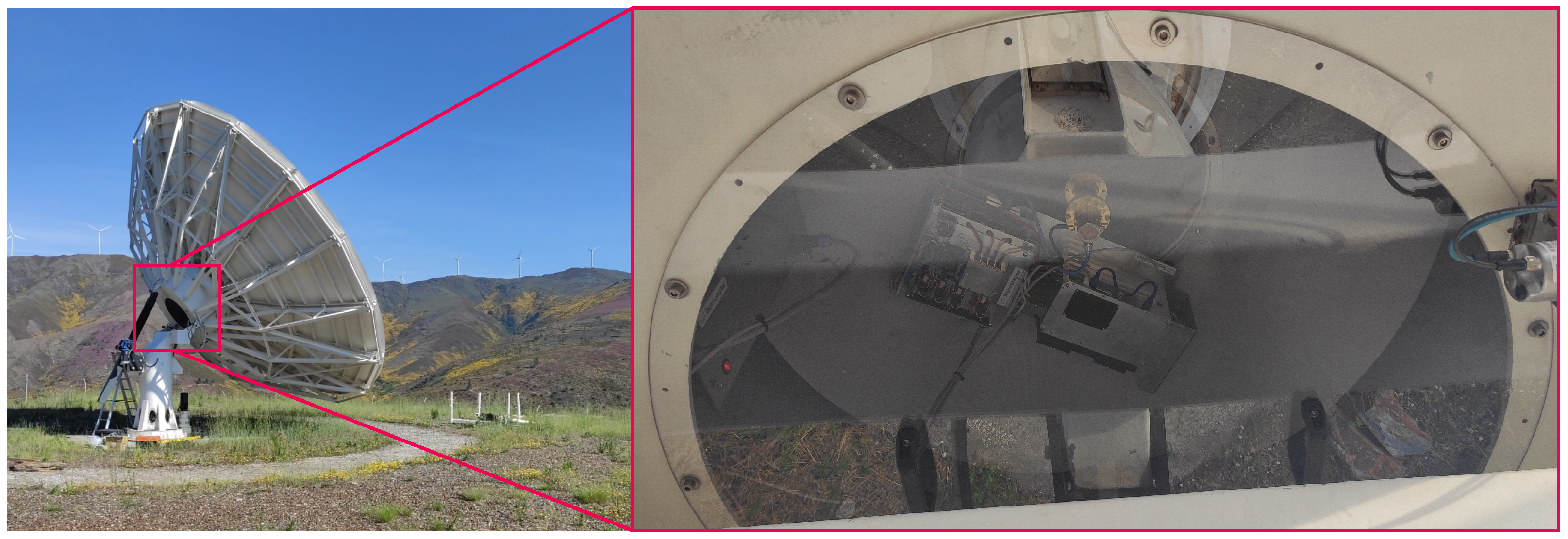
ATLAS was designed to consolidate national resources in preparation for the establishment of an SST sensor network. In 2019, Instituto de Telecomunicações initiated a major retrofit of its 9-m Cassegrain Antenna located in Pampilhosa da Serra Space Observatory (PASO), Portugal, to attach ATLAS, a complete radar system operating in the C-band (5.56 GHz) (Figure 1). A comprehensive technical overview of the system was presented in [5], accompanied by simulation studies on its expected operational performance. At the time of publication [5] in 2021, the generation and processing of the baseband signals were being thoroughly tested in a laboratory. These experiments led to several studies on the design of waveforms and signal processing chains for the system [5] (Section 4) [7]. The studies culminated in the first real-life scenario tests, where the whole system (except the antenna and power amplifiers) was tested in a setup with a major reflector at a well-defined distance [8].
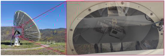
Figure 1.
Antenna located in PASO, with the radar system inside the hub.
After completing the preliminary functional tests in the lab and the field, we proceeded to the deployment phase. The deployment consisted of connecting the output of the power amplifier to the antenna feed through a polarizer. The polarizer underwent a matching procedure to maximize the isolation between the input/output ports and minimize reflections [9]. As part of the developments in 2022, we also presented the ATLAS Cloud Service API (ACSA) in [9]. ACSA enables monitoring and controlling of the radar through a web-based API, allowing the system to be accessed by multiple clients remotely. PASO houses many other sensors and systems [6,10], allowing ATLAS to act as a complete SST ground station with the following features:
- Monitoring and prediction of weather and sky conditions [11];
- Generation of schedules for optimal observation of a given catalog of space objects;
- Data fusion of optical and radar observations [12];
2.2. ATLAS: Technical Summary
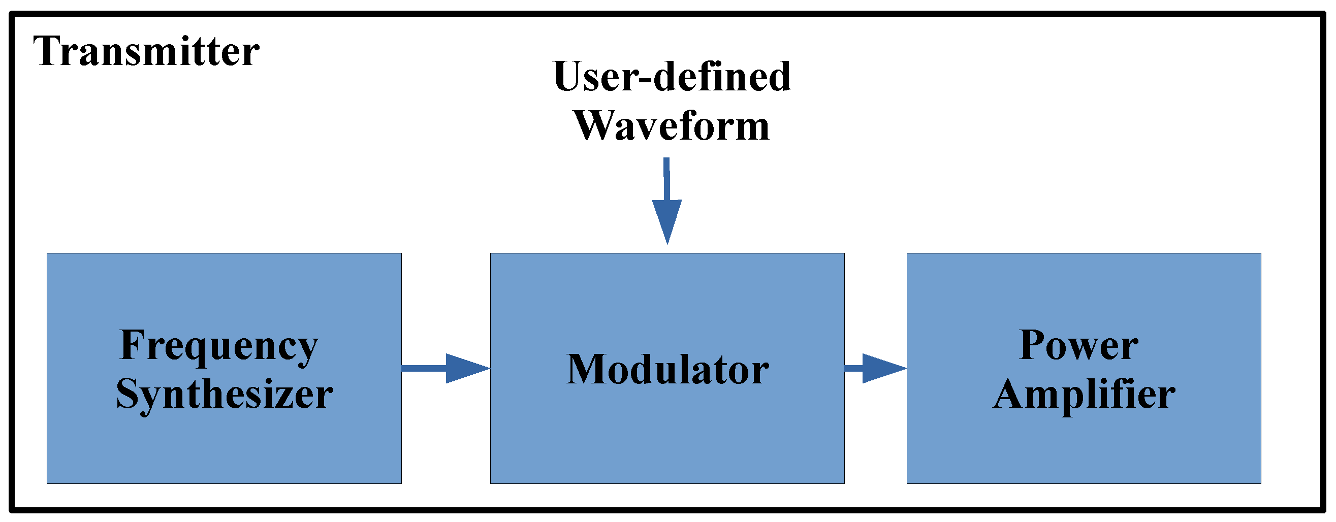
ATLAS is divided into a transmitting part and a receiving part. The transmitter, illustrated in a simplified depiction in Figure 2, is the subsystem responsible for generating and outputting the RF signal. Signal generation commences with a frequency synthesizer that generates the carrier frequency set at 5.56 GHz. This carrier signal is subsequently directed into a PIN modulator, which modulates the carrier in amplitude. The PIN modulator is controlled by a user-defined pulse shape. Following modulation, the signal proceeds to the power amplifier, where its peak power is adjustable within a range spanning from 155 W to 2 kW, facilitating versatile power configurations. For the observations shown in this article, the peak power was set to 1.6 kW. Table 1 summarizes all relevant parameters of the transmitter chain.
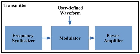
Figure 2.
Functional diagram of the transmitter subsystem.

Table 1.
ATLAS transmitter characteristics.
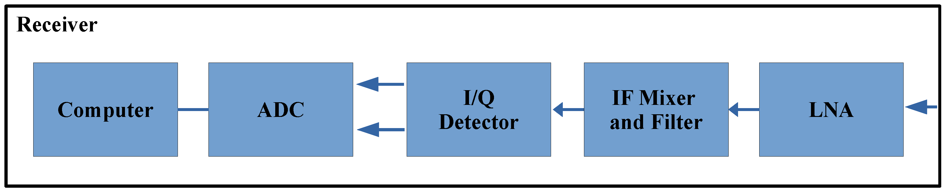
The receiver, depicted in Figure 3, includes an analog chain that is responsible for the demodulation and amplification of the received echoes. It starts with a low-noise amplifier (LNA), followed by a downconversion to a 400 MHz intermediate frequency (IF) and filtering (80 MHz of bandwidth). The local oscillator is provided by the same reference signal from the transmitter, guaranteeing a coherent conversion. The IQ detector converts the signal to a baseband and separates it into the I/Q components, which are then digitized at a maximum sample rate of 100 MS/s and stored in a computer for further processing. Table 2 summarizes all relevant parameters of the receiver chain.
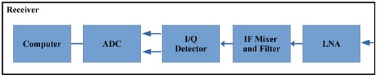
Figure 3.
Functional diagram of the receiver subsystem.
Table 2.
ATLAS receiver characteristics.
2.3. Space Object Tracking in LEO: Error Sources and Observation Strategy
Observing space objects in low Earth orbit (LEO) with a monostatic tracking radar is no trivial task due to the dynamics between the radar and the space objects and because of the multiple sources of error that arise. Tracking radars feature narrow beamwidths to increase the resolution and signal-to-noise ratio (SNR). On the other hand, objects in LEO have very high velocities [13]. These two facts make the window of opportunity for observation very short. Errors in both the pointing system and the orbit prediction can easily lead to missing objects.
The most complete source of orbital information is the US Two-Line Element (TLE) catalog. Given the sheer number of objects present in this catalog and the speed at which the orbital information is updated, the majority of SST stations, including ours, use it to perform predictions of the objects to observe.
The correct method for propagating TLE orbital data is by using an SGP propagator, with the most popular one being the SGP4 [14]. Although using TLE+SGP4 is a fast, convenient, and sufficient approach for other use cases, our experience suggests that it is less than ideal for uncooperative tracking in LEO given the errors associated with the usage of mean elements and simplified propagation models. Accuracy depends on sensor quality, data quantity, and space conditions, none of which are disclosed by the US Space Surveillance Network. ESA published a notable article, where it was estimated that TLE orbit errors in LEO were around 0.102 km (radial), 0.471 km (along-track), and 0.126 km (out-of-plane) [14]. These errors increase as we propagate further from the epoch, but it is difficult to quantify how much. TLE data do not include any information related to maneuvers, making it very difficult to predict a satellite’s position after one. The history of the TLE sets of a given object can be used to understand whether it has undergone maneuvers, which can be useful information when dealing with uncooperative satellites [15].
Inaccurate geo-referencing of the antenna homing system may lead to biases in the azimuth and elevation measurements. Once the homing system is correctly geo-referenced, a finer calibration can be performed using celestial sources like the Sun/Moon to further decrease the offset errors [16]. Periodic calibration routines involving celestial sources should be performed to ensure the pointing system remains accurate.
The selection of resident space objects (RSOs) to track during the calibration phase can also play an essential role in mitigating these sources of error. The International Space Station (ISS) serves as an ideal candidate for initial measurements due to its significantly large Radar Cross-Section (RCS), approximately 400 m2, and its ability to orbit within the lower LEO region (below 500 kilometers in altitude), resulting in the reception of higher-energy echoes compared to other RSOs. Position and velocity state vectors for the ISS are provided by NASA and are publicly available [17,18]. These vectors are listed at four-minute intervals over the last 15 days, and during maneuvers, the vectors are reported at two-second intervals [18]. The ephemeris files also contain other important information, such as the mass of the ISS, drag area, drag coefficient, solar radiation area, and solar radiation coefficient, allowing orbit propagation with special perturbation techniques [19].
Other LEO operational satellites such as CRYOSAT-2 and Jason-3 are equipped with telemetry and retroreflectors, which provide precise ephemeris information [20]. This information can be used for highly accurate predictions of their passages, offering valuable data for both calibration procedures and evaluating the performance of ground-based sensors [21]. Passive calibration satellites, like STELLA and STARLETTE, were designed to have high reflectivity and spherical shapes, ensuring that their RCS remains independent of the viewing angle [22]. They play a critical role in fine-tuning RCS measurements obtained by the sensors, as they provide a reliable reference point for RCS values.
In light of the foregoing discussion, the following are some key ideas that every SST ground station should be aware of:
- Use the most recent TLE sets available to reduce propagation errors and unaccounted maneuvers;
- Perform regular calibration routines using celestial sources;
- Use well-behaved satellites that provide precise ephemeris information and/or constantly updated TLEs to refine the pointing system;
Finally, the observation strategy used can also help mitigate some of the aforementioned errors. We suggest implementing a semi-surveillance approach. This approach entails positioning the antenna at a predicted location in the sky for the target satellite and illuminating it both before and after the expected time of the object’s passage within the antenna’s beamwidth. By adopting this method, the likelihood of successfully capturing the target increases, and the resulting echoes yield valuable insights into how to rectify discrepancies in orbit predictions and offsets of the system. By assuming a symmetric illumination time before and after the expected time of passage, it is expected that the echoes will appear centered around the middle of the illumination time window. By assuming a range acquisition window centered on the object’s expected range, the echoes are expected to appear centered in the range window. Deviations from the center of the range-pulse map can be used to compensate for pointing, timing, and orbit prediction errors.
2.4. Calibration Procedure
Calibration of both the radar performance and the pointing system requires well-characterized and stable sources of electromagnetic energy, preferably located in the far-field region of the antenna. The far field of an antenna is the distance from the source necessary to approximate the electromagnetic wavefronts as approximately planar [23] (Chapter 1). This condition is met if the distance from the source to the aperture is at least . This approximation is typically used as a condition in the radar equation, so we need to ensure that targets are in this region. The far-field distance of ATLAS is approximately 3 km, so we consider all satellites in orbit and celestial bodies (including the Sun) to meet this criterion.
The use of EM energy from the Sun is a well-established method for checking antenna alignment and receiver sensitivity, and it is quite common for manufacturers to provide Sun calibration tools as part of their software packages. In [24], the authors presented a method for locating the Sun’s coordinates and determining the pointing offsets. A method for determining the true elevation of a target using observations of the Sun was introduced in [25]. In [26], the authors presented an improved method for pointing calibration with the Sun using operational weather radar scans made at very low elevation angles. When calibrating radar using the Sun, the radar is, in fact, used as a radiometer. The transmitter is not used since we expect no echo from the Sun due to its distance from the Earth [27]. Because of this, only the receiving chain can be calibrated using the Sun, and to calibrate the whole system, other techniques have to be used, such as the ones explained in Section 2.3.
The Sun is one of the preferred candidates for calibration because of the following:
- It can be regularly observed from any point on Earth;
- Its position in the sky can be precisely calculated at any time and location [26,28];
- It radiates at all wavelengths, and the radiation is generally unpolarized [29];
- The solar flux incident on the Earth’s surface varies between 100 and 300 solar flux units. The solar flux is measured constantly by many stations worldwide, and these measurements are public;
The diameter of the Sun in the visible wavelengths is approximately 695,700 km, as defined by the International Astronomical Union (IAU) [30], which results in an apparent arc of approximately 0.53°. At centimeter wavelengths, this value is different, and an effective RF diameter can be obtained [31]. For ATLAS’s operating frequency, the Sun can be considered a homogeneous disc with a diameter of approximately 0.57° [27] (and the references therein).
It is common to use the horizontal coordinate system [32] when working on a radar ground station. This system uses the station’s (observer’s) local horizon as the plane to define two angles: azimuth and elevation. Azimuth is the angle around the horizon; it starts at 0° at true north and increases eastward. Elevation is the angle above the horizon starting at 0° at the horizon and increasing until 90° at the zenith, for visible objects. The horizontal coordinate system is always referenced to the station position, which is the origin, so to obtain the position of the object referenced to the Earth, the location of the station on the Earth is necessary. The equations for the elevation and azimuth calculations of the Sun are:
where and are the elevation and azimuth of the Sun, respectively. is the declination of the Sun, is the latitude of the ground station, and is the hour angle of the Sun. The up-to-date declination and hour angle of the Sun are made public by many observatories. The elevation angle is affected by changes in the refractivity of the atmosphere with altitude. The authors of [28] provided an extensive explanation of the equations necessary for calculating the refractivity index and compensating for the apparent elevation obtained in (1). These equations usually require access to local meteorological parameters such as ambient temperature and pressure. The effect of refraction should be taken into account, especially when collecting data at low elevations (<10 deg [26]).
Measurement of solar noise is a relatively straightforward, accurate, reproducible, and convenient method for assessing receiver performance. It consists of measuring the ratio between the power received by the antenna when pointed at the Sun and when pointed at the cold sky [33]. This metric proves valuable in receiver optimization because a higher measured solar noise correlates with improved G/T, allowing for the detection of weaker signals.
The basic principle of pointing calibration with the Sun consists of scanning the azimuth/elevation positions around the predicted position of the Sun and measuring the received power [16]. When the antenna is pointing to the center of the solar disk, it will receive the maximum power. The difference between the sensor angle readings at the peak power and the predicted position of the Sun corresponds to the bias in the positioning system.
The cross-scanning routine consists of the following steps:
- 1.
- Define a vector of N offset angles .
- 2.
- Define a vector of N time instants .
- 3.
- Predict the azimuth positions of the Sun for the defined time instants: .
- 4.
- Compute the scanning positions: .
- 5.
- Point the antenna to positions S at time instants T and compute the power received for each position.
- 6.
- Locate the peak power and update the offset with the new angle value.
- 7.
- Repeat for the elevation angle.
The scan should be performed by alternating between azimuth and elevation to avoid the coupling error of moving azimuth and elevation simultaneously and for several iterations until the obtained offsets converge within a given uncertainty. This routine ensures that the calculated positions compensate for the Sun’s movement during the scan. The operator should make sure the timestamps between points are long enough to be able to move the antenna and record the signal at the correct time.
This method should only be used when the beamdwith is larger than the diameter of the Sun. In cases where the beamwidth is larger, the scanning will return the beam pattern of the antenna, and we can confidently say that the maximum noise reading corresponds to the center of the Sun. However, if the beamwidth is smaller than the diameter of the Sun, there will be multiple maximum values when passing inside the solar disk, which will result in a beam pattern with a flat top instead of a peak.
2.5. Signal Model
Let us consider a radar system emitting a pulse with a carrier at frequency , modulated with a complex baseband linear frequency modulation (LFM)
where is the pulse duration, t is the fast time, B is the signal bandwidth, and . Now let us assume that the radar is illuminating a target with a constant radial velocity, causing the range to change according to
where is the slow time, is the initial range, is the radial velocity, and CPI is the coherent processing interval. The slow time can be written as dependent on the pulse number
where is the pulse repetition interval, and M is the number of pulses in a CPI.
If the radar emits a burst of identical pulses, given by (3), the received echoes after carrier demodulation are given by
where is the complex amplitude of the echo, c is the speed of light, , and is the additive noise term. The sources of noise arise from inside and outside a circuit: solar noise, cosmic and galactic noise, interference from other antennas, and instrumental noise. Different noise sources are modeled by different distributions, with the most predominant one being thermal noise [23] (Chapter 1), which is white and follows a normal distribution in amplitude. Given that the final noise signal is a byproduct of interference from potentially many different sources, the Central Limit Theorem can be applied, and it is reasonable to assume additive white Gaussian noise (AWGN) with a zero mean and a variance : .
After passing the signal through a matched filter, the target’s echoes are given by
where is the complex amplitude of the compressed echoes, and is the range. Equation (7) contains a sinc term [23] (Chapter 20), which is centered at and migrates during the CPI.
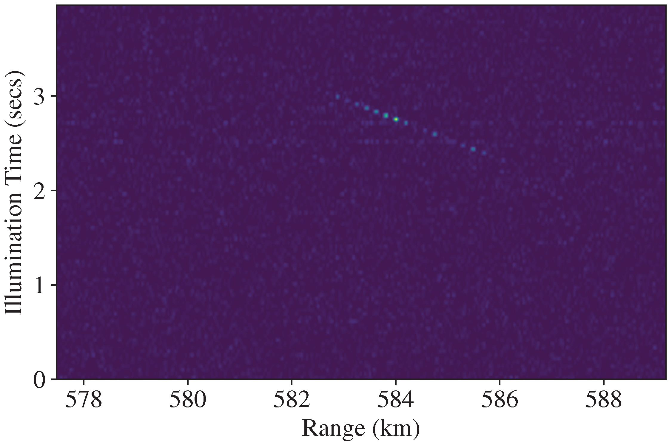
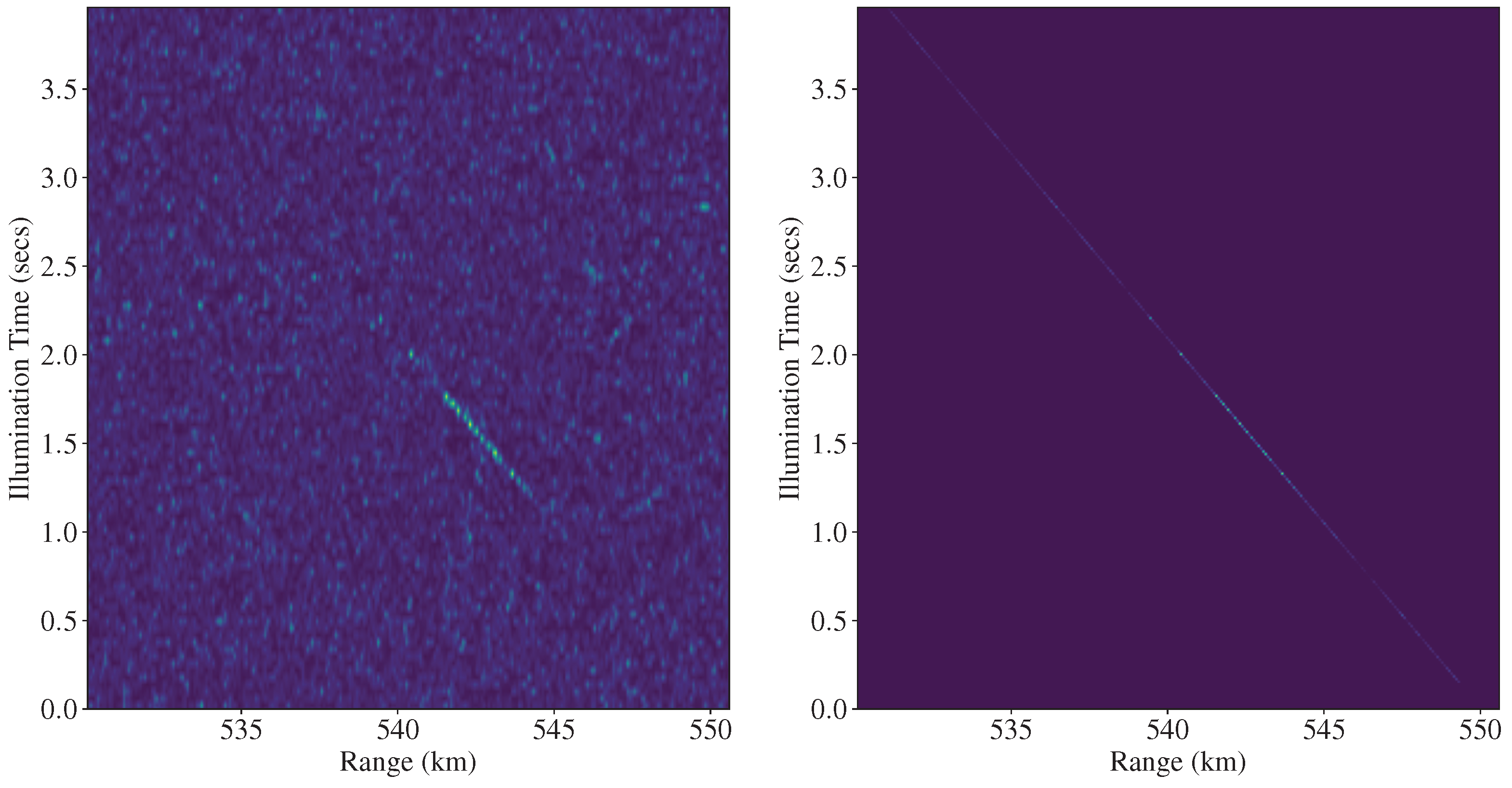
Real examples of the signal model in Equation (7) are presented in Figure 4 and Figure 5 ( is the range axis, and is the Illumination time axis). These figures correspond to the squared magnitude of the pulse-compressed echoes received during the observation of two satellites. In both cases, it is possible to see a distinct line that corresponds to range migration during the illumination time.

Figure 4.
NORAD ID: 25544, ISS. A streak is formed by the echoes received from the sattelite.
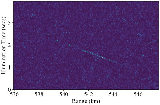
Figure 5.
NORAD ID: 54216, CSS (MENGTIAN). A streak is formed by the echoes received from the sattelite.
The complex exponential term at the end of Equation (7) can be developed into
where is the Doppler shift. The sequence of phase-change terms along the slow time forms a complex sinusoid at the Doppler frequency and is sometimes called the spatial Doppler signal.
2.6. Signal Processor
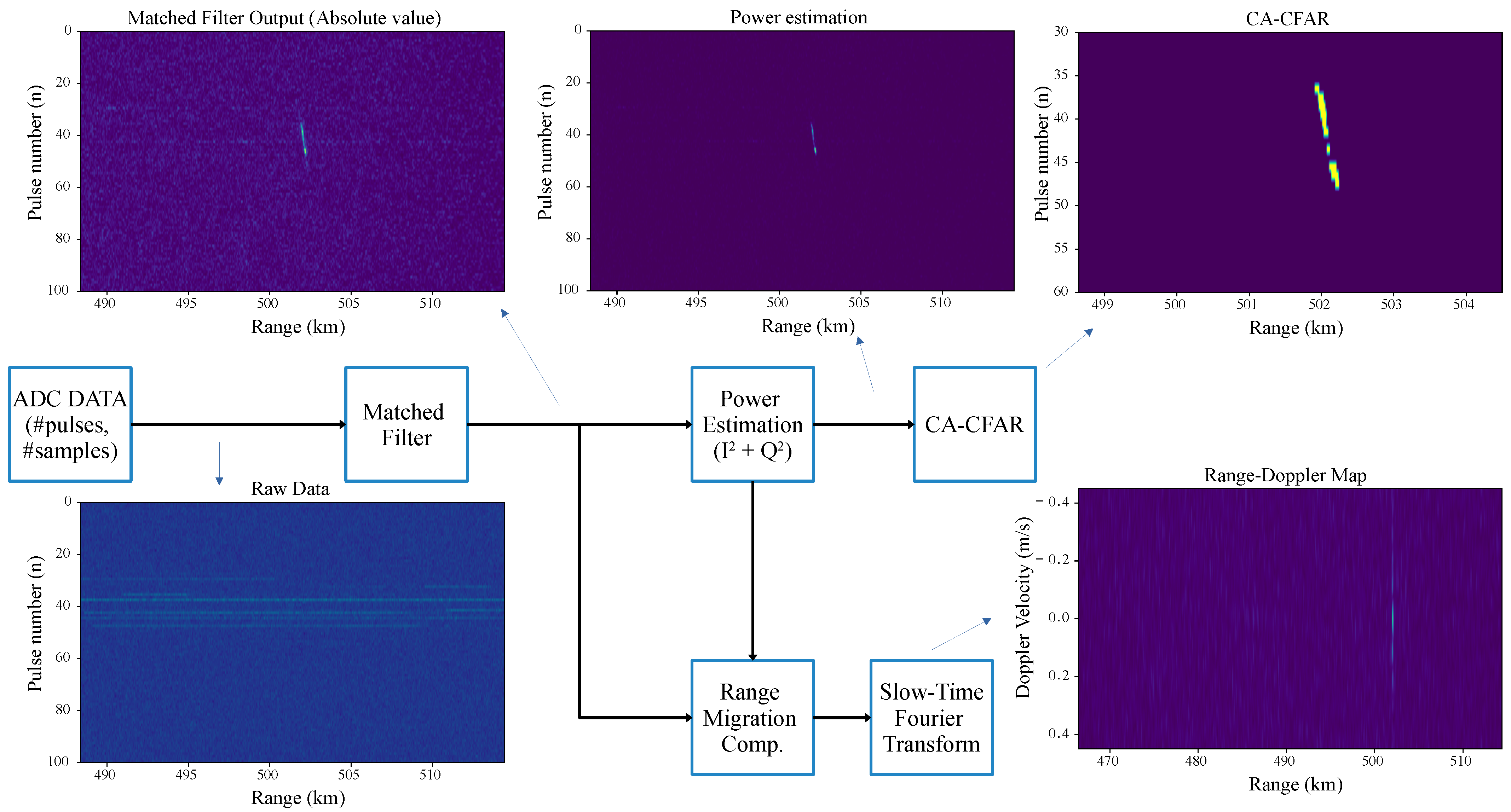
ATLAS uses an AM Chirp waveform with a bandwidth of 2 MHz and emits bursts of 100 pulses at a frequency of 33 Hz. This configuration results in a range resolution of 75 m after pulse compression and a Doppler resolution of 0.009 m/s. The maximum unambiguous range is 4545 km, and the maximum unambiguous velocity is 0.44 m/s. The signal processor is depicted in Figure 6. The raw data acquired by the ADCs for each pulse are stacked in a range-pulse complex matrix [34] (Chapter 3). The complex data are processed by a matched filter [34] (Chapter 4) and then split into two branches.
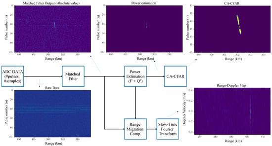
Figure 6.
ATLAS signal processor. The output of the signal processor consists of a list of detections containing range and velocity information.
The first one computes the sample power and passes the signal through a cell-averaging constant false-alarm ratio (CA-CFAR) [34] (Chapter 6) detector with a probability of false alarm of . At the end of this branch, a list of range detections is obtained. The second branch compensates for range migration and performs pulse-Doppler processing.
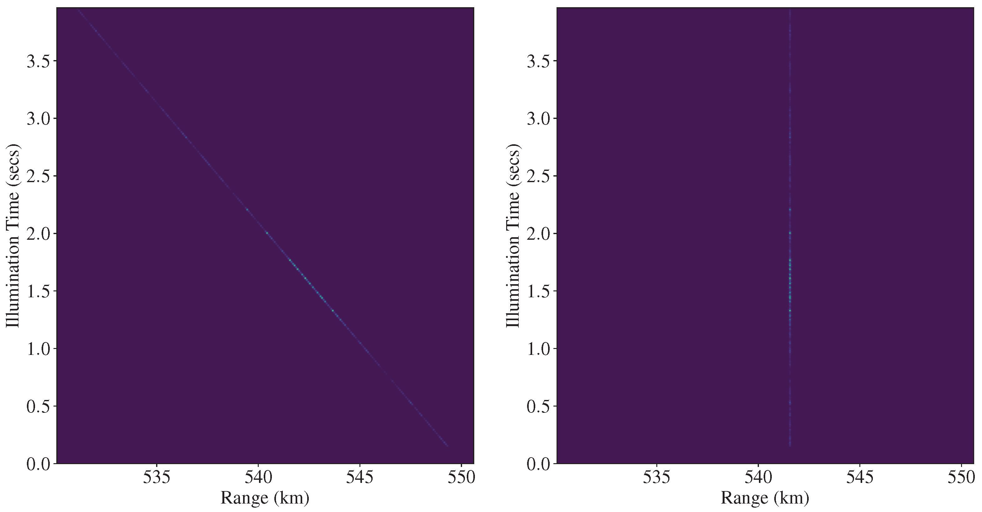
Range migration compensation is achieved using the Radon transform (RT) for line detection [35] and envelope cross-correlation for range alignment [36,37]. The RT of a function is defined as [38]
where p is the slope of the line and is its intercept with the y-axis. So, is the line integral of over the line defined by the parameters p and . By applying the RT across a range of slopes and intercepts with the y-axis, we obtain the sinogram of , which contains maximums for the pairs of that define existing lines in the domain.
By combining (7) and (9), it is possible to obtain the RT of the received signal in terms of the range and the radial velocity
where is the pulse repetition interval, and is the range resolution.
The radial velocity can also be defined as the anticlockwise angle from the slow time axis to the range walk line
If there is one line in , it can be detected using
where and are estimates for the initial range and radial velocity computed with the RT. After detecting the line, we can filter out the rest of the components in the sinogram (by setting them to 0) and apply the inverse Radon transform (IRT), resulting in the detected line being isolated, denoted as

Figure 7.
Line detection based on the Radon transform applied to an observation of CSS (MENGTIAN).
Applying the envelope cross-correlation to estimates the range cell shift between the peaks in the line, which are then used to align the predominant scatterer within the same range bin, as depicted in Figure 8.
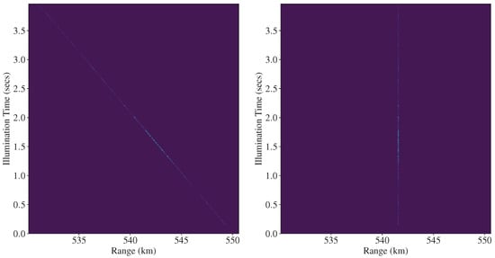
Figure 8.
Range alignment of the observation shown in Figure 7.
Now that the range alignment is completed, we need to correct for the Doppler term (Equation (8)). To do this, we can implement a filterbank, with each filter tuned to a different Doppler frequency. This can be obtained by applying the Fourier transform along the slow time, generating a range-Doppler map [34] (Chapter 5). Due to the usage of a low PRF, the Doppler velocity obtained is highly ambiguous. Unambiguous velocity estimation is obtained from the line parameters found with the RT.
3. Results
3.1. Calibration
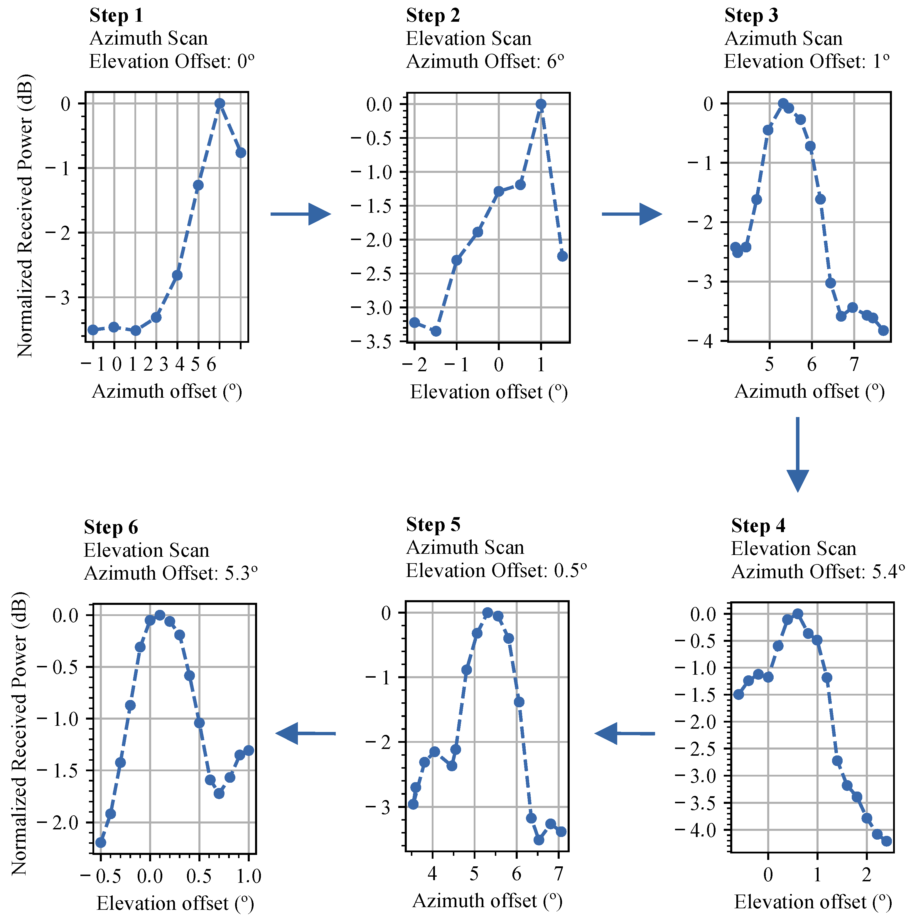
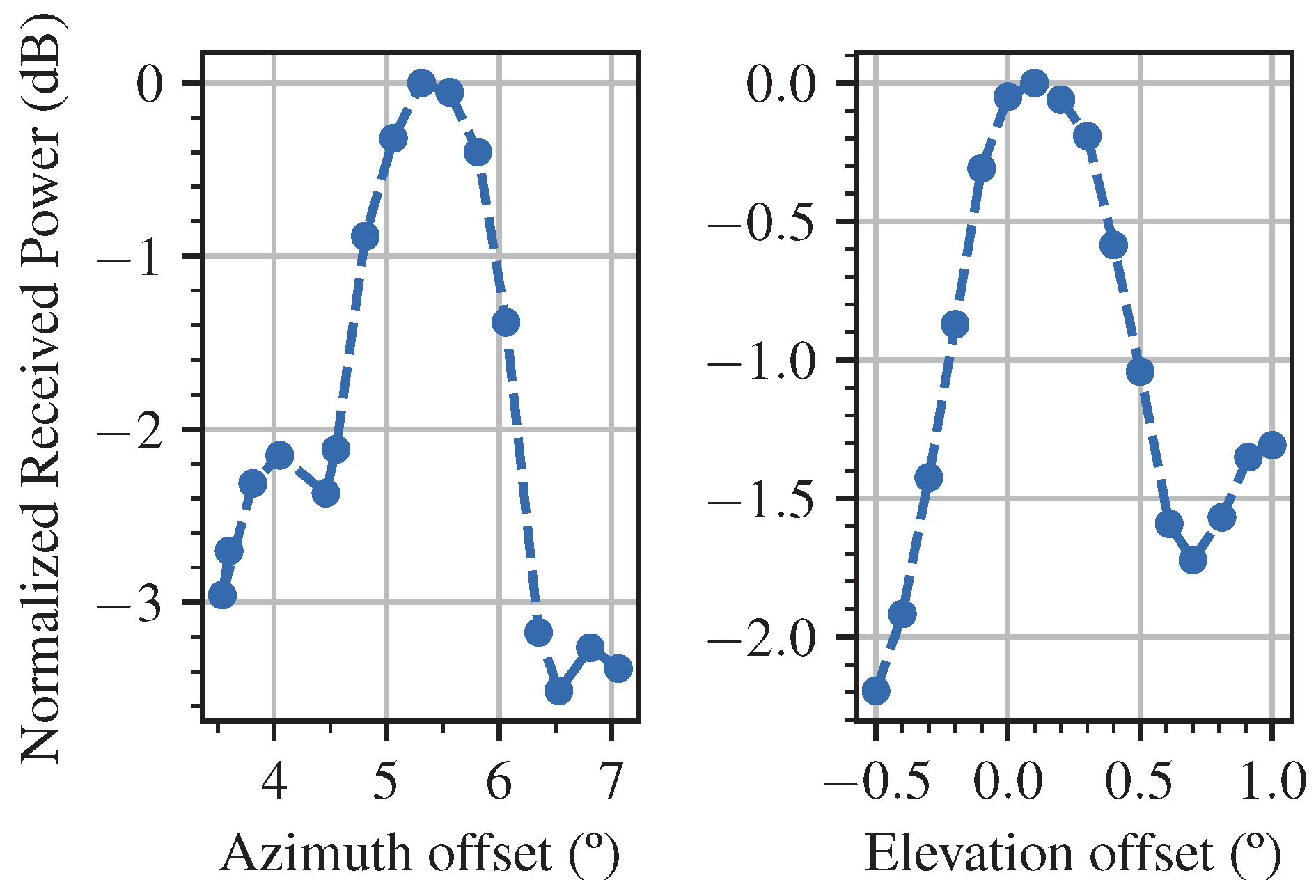
The results from the last calibration procedure with cross-scanning using the Sun are depicted in Figure 9 and Figure 10. Figure 9 showcases some of the steps of scanning. Initially, an azimuth scan with an 8° searching angle yielded an offset estimate of 6°. Then, an elevation scan with a 4° searching angle provided an initial estimate of 1°. Subsequently, finer-resolution scans were conducted around these initial offsets, and the azimuth offset was corrected to 5.4°, and the elevation offset was corrected to 0.5°. The convergence was obtained after the offset in azimuth stabilized within an uncertainty of 0.2° and the offset in elevation stabilized within an uncertainty of 0.05°. The results in Figure 10 correspond to the last iteration on each axis after convergence was obtained.
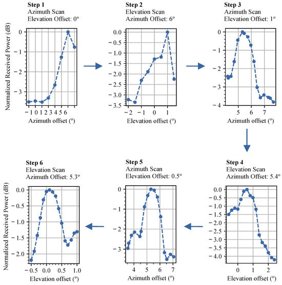
Figure 9.
Example of the steps of the calibration procedure. In Step 1, an azimuth scan was performed with an 8° searching angle to obtain an initial guess of the offset, where a peak was obtained at 6°. In Step 2, the 6° offset in azimuth was fixed, and an elevation scan was performed with a 4° searching angle to obtain an initial guess of the offset, where a peak was obtained at 1°. Once an initial guess for both offsets was obtained, the same process was repeated but with finer resolution around the new offsets (Steps 3 and 4), where the azimuth offset was corrected to 5.4° and the elevation offset was corrected to 0.5°. The process converged in Steps 5 and 6, as detailed in Figure 10. The number of scans required until convergence may vary, and for illustration purposes, intermediary scans were omitted.
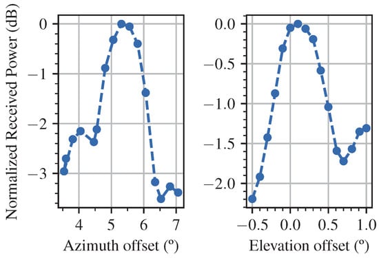
Figure 10.
Offsets obtained for azimuth and elevation after convergence in the cross-scanning procedure. The azimuth offset is 5.3 ± 0.2°, where the mainlobe can be identified roughly in the region between 4.9° and 5.7°, the left sidelobe is visible between 3.5° and 4.5°, and the right sidelobe is between 6.5° and 7° (incomplete). The elevation offset is 0.10 ± 0.05°, where the mainlobe can be identified roughly in the region between −0.27° and 0.47°, and the right sidelobe is between 0.6° and 1° (incomplete).
3.2. Space Object Observations
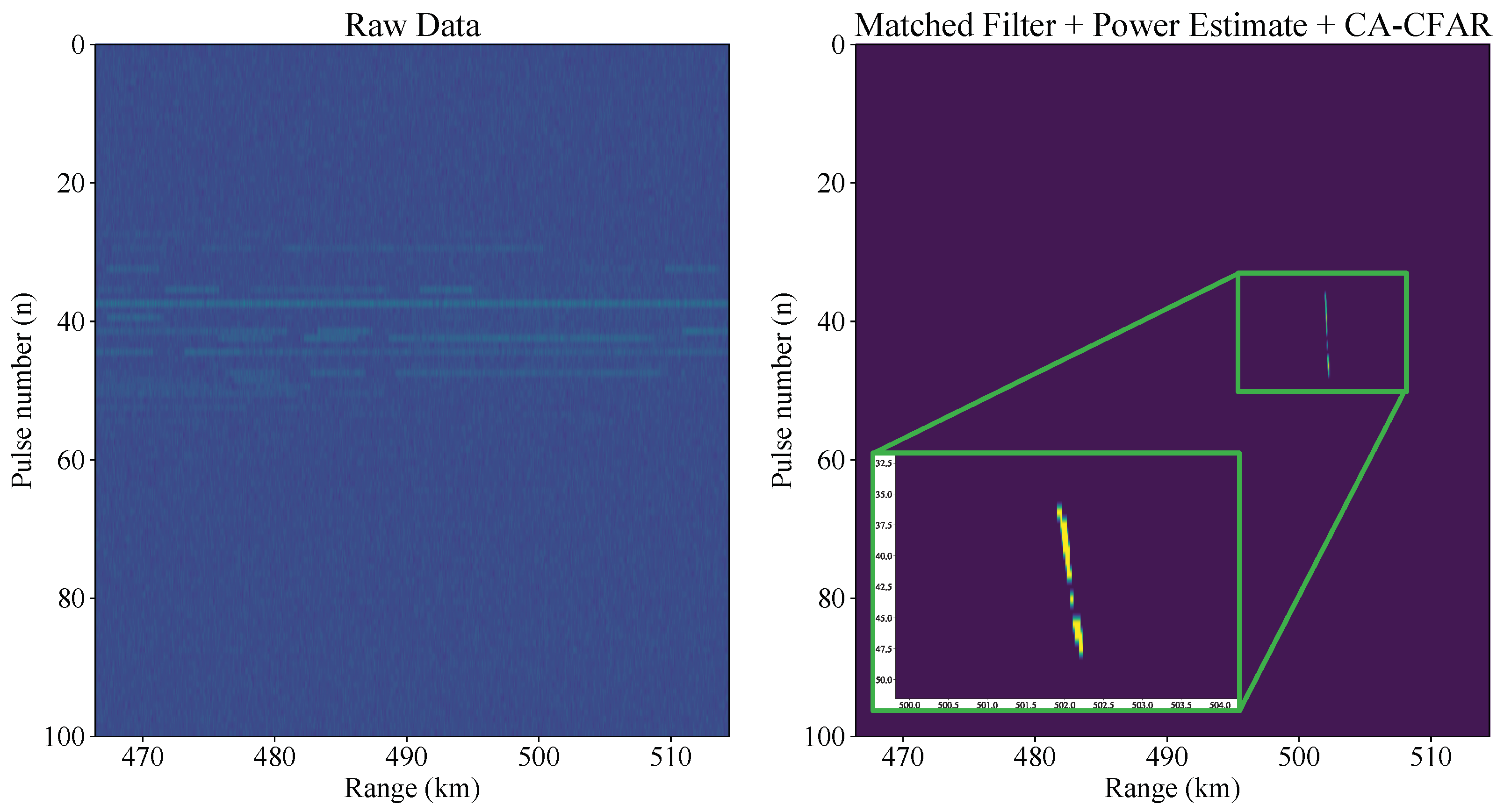
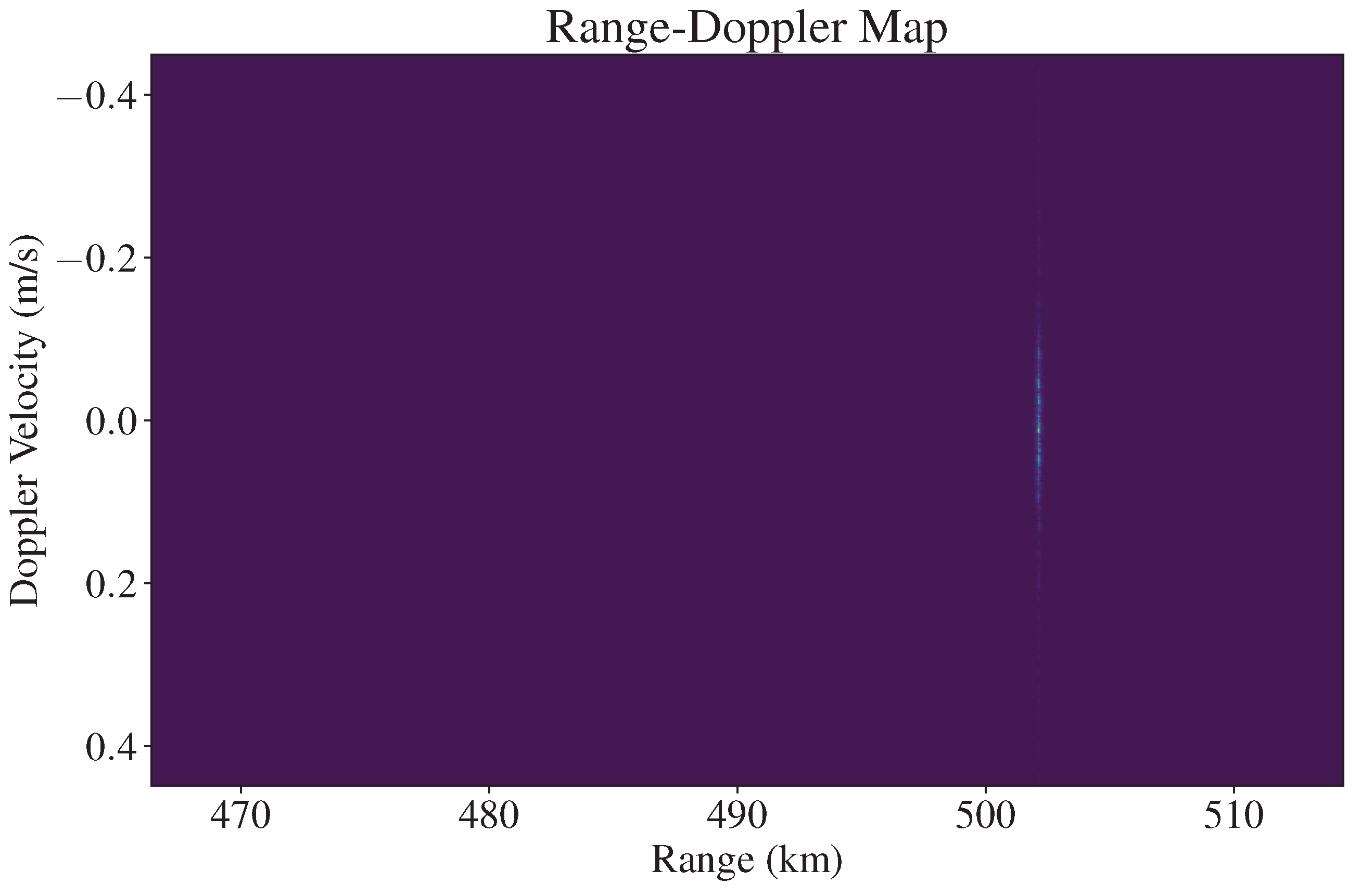
The observations presented in this section resulted from the first campaign of observations performed with ATLAS in July 2023 and a second campaign during the last week of January 2024. The preferred candidate for observation was the ISS, as explained in Section 2.2. Figure 11 showcases one of the observations obtained. After applying the signal processing chain to the raw data, a streak of detections is visible. The object returned reflections from pulses 35 to 48 out of the 100 pulses emitted. Range migration is obvious given that the object moved to other range cells from pulse to pulse. Figure 12 depicts the range-Doppler map obtained for the observation in Figure 11.
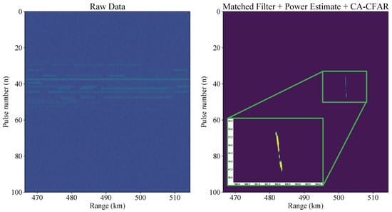
Figure 11.
Image on the left shows the absolute value of the complex raw data recorded by the ADCs. The image on the right shows the detections obtained. The detections cluster into a streak, a common pattern when observing space objects due to the effect of range migration.
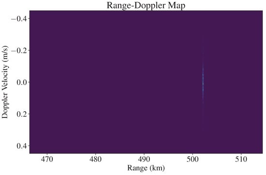
Figure 12.
Range-Doppler map with detection at 502.0 km of range and 0.014 m/s of Doppler velocity.
A total of 35 range detections and 5 velocity detections were obtained from the campaign. Table 3 shows the complete data for some of the observations. The rest of the observations were used to assess the performance of the system, as explained in Section 4.2.
Table 3.
Some examples of observations.
4. Discussion
4.1. Calibration
Figure 10 shows not only the offset of the main beam but also the shape of the main beam and sidelobes. The sidelobes of the antenna are not symmetric and require re-alignment. This is due to it being an old antenna that was moved and underwent several upgrades and repairs over the years. A 3D point cloud was recently obtained using LIDAR, showing that the feed and the secondary reflector are aligned, but some of the panels of the main reflector are misaligned, compromising the parabolic shape. This issue is currently being addressed.
4.2. Revisiting the Radar Equation
By adapting one of the many forms of the radar equation, the single pulse signal-to-noise ratio () after pulse compression is given by [39]:
where is the transmitted peak power (W), G is the antenna gain, is the operating wavelength (m), is the target radar cross-section (RCS) (), is the pulse width (s), is the bandwidth of the waveform (), R is the distance to the object (m), is the noise factor of the receiver, k is the Boltzmann constant (), T is the receiver temperature (K), B is the bandwidth of the receiver (), and accounts for all losses.
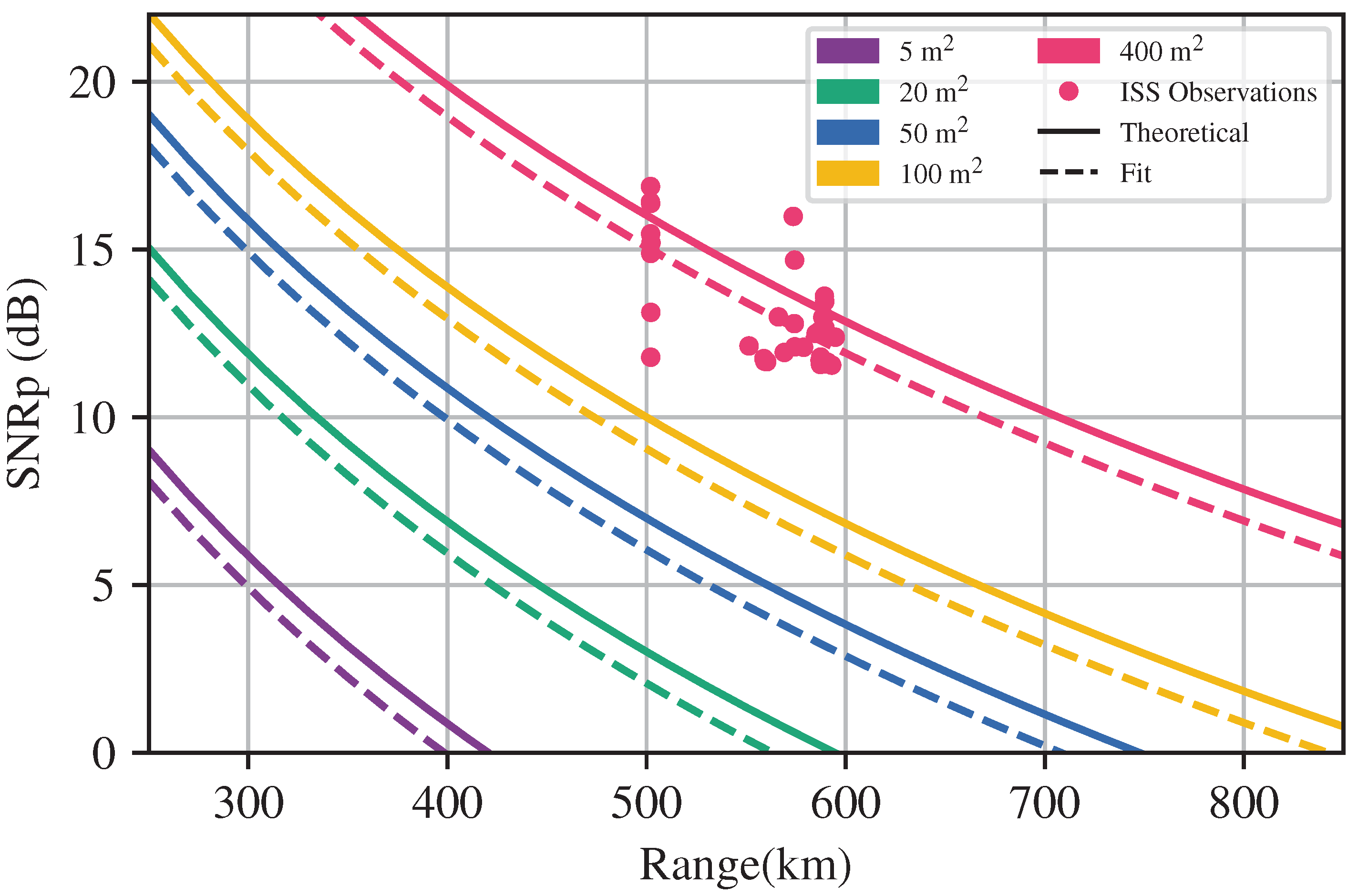
The loss term represents all the factors that are difficult to obtain/identify, e.g., system losses and atmospheric losses. While an educated guess can be a useful starting point to evaluate the future performance of a radar system, ideally, this term should be updated by performing measurements with the system. Figure 13 represents the theoretical curves obtained for ATLAS for different RCS values, represented as solid lines. Since we have now made observations of the ISS, we decided to use these to revisit the equation and improve it. To do this, we fixed the equation terms for an RCS of 400 m2 and fitted the loss term to the observations using a non-linear least-squares method. The fitting resulted in an of 15.94 dB with a variance of 6.09 dB. The fit curves are represented as dashed lines. The variance of the estimate is high due to the dispersion and number of measurements. We can see that for ranges around 500 km, the detections have variations of around 5 dB in the SNR, which can be due to many factors such as the scintillation of the object or variations in the gains of the system during pulse emission/reception. We are currently investigating the cause of these differences in the SNR for the same range and RCS. Currently, the number of observations is limited, and the objective is to gather more observations at different ranges and RCSs to obtain a better estimate of .
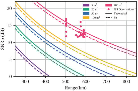
Figure 13.
SNR dependence on the range for different RCSs. The theoretical curves (solid lines) were adjusted using the ISS observations to obtain a better estimate of the performance of ATLAS in real scenarios (dashed lines).
5. Conclusions and Future Work
After 4 years of development, testing, and validation, the ATLAS system has successfully achieved its first uncooperative observations of space objects. These results were only possible due to the efforts invested in creating an adequate observation strategy, implementing calibration techniques, and exploring the capabilities of the system in terms of baseband waveform generation and processing.
As of now, ATLAS is evolving to be not only a radar system but a fully-fledged SST ground station with the capacity for orbit prediction, schedule generation, and maintenance of an internal catalog. ATLAS is still a work in progress that is moving closer to being used in an operational scenario. Ongoing and future work comprises the following:
- Obtain more observations of well-known objects at different ranges and RCSs to obtain a better estimate of the radar’s performance;
- Compare range and range-rate measurements with precise ephemeris to correct unaccounted bias terms;
- Increase the probability of detection by designing more sophisticated detectors. This includes exploring subspace detector design [40,41], multi-stage adaptive detectors [42,43], and machine learning-based detectors [44,45];
- Address ambiguous Doppler velocity extraction using multiple PRFs [46,47];
- Increase the peak power, bandwidth, and PRF of the system to increase the SNR, range resolution, and Doppler resolution.
Author Contributions
Conceptualization, J.P., M.B. and P.M.; methodology J.P., M.B. and P.M.; software, J.P.; validation, M.B., P.M. and B.C.; formal analysis, J.P., M.B., P.M. and B.C.; investigation, J.P., M.B., P.M. and B.C.; resources, J.P.; data curation, J.P. and B.C.; writing—original draft preparation, J.P.; writing—review and editing, M.B., P.M., B.C., D.B. and M.F.; visualization, J.P.; supervision, P.M. and M.B.; project administration, D.B. All authors have read and agreed to the published version of the manuscript.
Funding
This work was supported by the Fundação para a Ciência e Tecnologia (FCT), Ph.D. grant No. 2022.12341.BDANA.
Data Availability Statement
Data were obtained from the Portuguese Ministry of Defense and are available from the corresponding author with the permission of the Portuguese Ministry of Defense.
Acknowledgments
The team acknowledges the European Commission’s Horizon 2020 Programme under the Space Surveillance and Tracking (SST) grant agreement 2-3SST2018-20. Additionally, the team acknowledges LC Technologies for their technical developments in close collaboration with Instituto de Telecomunicações. We also acknowledge the support from the European Regional Development Fund (FEDER) through the Competitiveness and Internationalization Operational Programme (COMPETE 2020) of the Portugal 2020 framework (Project SmartGlow with No. 069733 (POCI-01-0247-FEDER-069733)). The team further acknowledges the support from the ENGAGE-SKA Research Infrastructure, Ref. POCI-01-0145-FEDER-022217, funded by COMPETE 2020 and FCT, Portugal. IT team members acknowledge the support from Projecto Lab. Associado UID/EEA/50008/2019. Finally, the team acknowledges the Portuguese Ministry of Defense for allowing the usage and dissemination of the results.
Conflicts of Interest
Authors M.B. and B.C. are employed by ATLAR Innovation. The remaining authors declare that the research was conducted in the absence of any commercial or financial relationships that could be construed as a potential conflict of interest.
Abbreviations
The following abbreviations are used in this manuscript:
| SSA | Space Situational Awareness |
| SST | Space Surveillance and Tracking |
| ESA | European Space Agency |
| NASA | National Aeronautics and Space Administration |
| EUSST | European Space Surveillance and Tracking |
| ATLAS | rAdio TeLescope pAmpilhosa Serra |
| PASO | Pampilhosa da Serra Space Observatory |
| ACSA | ATLAS Cloud Service API |
| LEO | Low Earth Orbit |
| SGP | Simplified General Perturbation |
| SNR | Signal-to-Noise Ratio |
| PRF | Pulse Repetition Frequency |
| TLE | Two-Line Element |
| RSO | Resident Space Object |
| ISS | International Space Station |
| RCS | Radar Cross-Section |
| MDPI | Multidisciplinary Digital Publishing Institute |
| LIDAR | Light Detection and Ranging |
| ADC | Analogue-to-Digital Converter |
References
- ESA’S Annual Space Environment Report; Technical report; ESA Space Debris Office: Darmstadt, Germany, 2023.
- United Nations Office for Outer Space Affairs. Treaty on Principles Governing the Activities of States in the Exploration and Use of Outer Space, including the Moon and Other Celestial Bodies. Available online: https://www.unoosa.org/oosa/en/ourwork/spacelaw/treaties/introouterspacetreaty.html (accessed on 8 January 2021).
- European Space Agency. SSA Programme Overview. Available online: https://www.esa.int/Space_Safety/SSA_Programme_overview (accessed on 12 February 2024).
- EU SST. Eusst-European Space Surveillance and Tracking Projects. Available online: https://www.eusst.eu (accessed on 12 February 2024).
- Pandeirada, J.; Bergano, M.; Neves, J.; Marques, P.; Barbosa, D.; Coelho, B.; Ribeiro, V. Development of the First Portuguese Radar Tracking Sensor for Space Debris. Signals 2021, 2, 122–137. [Google Scholar] [CrossRef]
- Coelho, B.; Barbosa, D.; Bergano, M.; Correia, A.; Freitas, J.; Marques, P.; Pandeirada, J.; Ribeiro, V. New SST optical sensor of Pampilhosa da Serra—Studies on image processing algorithms and multi-filter characterization of space debris. In Proceedings of the 8th European Conference on Space Debris (Virtual), Darmstadt, Germany, 20–23 April 2021; ESA Space Debris Office: Darmstadt, Germany, 2021; pp. 1–4. [Google Scholar]
- Pandeirada, J.; Bergano, M.; Marques, P.; Barbosa, D.; Freitas, J.; Ribeiro, V. Design of Pulsed Waveforms for Space Debris Detection with Atlas. In Proceedings of the 8th European Conference on Space Debris (Virtual), Darmstadt, Germany, 20–23 April 2021. [Google Scholar]
- Pandeirada, J.; Bergano, M.; Marques, P.; Barbosa, D.; Coelho, B.; Ribeiro, V.; Freitas, J.; Nunes, D.; Eduardo, J. A Portuguese radar tracking sensor for Space Debris monitoring. arXiv 2022, arXiv:2111.02232. [Google Scholar] [CrossRef]
- Pandeirada, J.; Bergano, M.; Marques, P.; Barbosa, D.; Coelho, B.; Freitas, J.; Nunes, D. ATLAS: Deployment, Control Platform and First RSO Measurements. arXiv 2023, arXiv:2211.03586. [Google Scholar] [CrossRef]
- Gonçalves, L.F.P. Space Data Processing Pipeline for PASO (Pipeline de Análise de Detritos Espaciais Para o PASO). Master’s Thesis, University of Aveiro, Aveiro, Portugal, 5 July 2023. [Google Scholar]
- Gonçalves, L.F.P.; Sousa, A. CLOWN: A new tool for cloud detection with an All-Sky camera for optimization of space-debris surveys. In Proceedings of the 73rd International Astronautical Congress (IAC), Paris, France, 18–22 September 2022. [Google Scholar]
- Coelho, B.; Barbosa, D.; Berganoa, M.; Pandeirada, J.; Marques, P.; Correia, A.C.M.; Freitas, J.M.d. Developing a data fusion concept for radar and optical ground based SST station. In Proceedings of the 73rd International Astronautical Congress (IAC), Paris, France, 18–22 September 2022; International Astronautical Federation: Paris, France; pp. 1–3. [Google Scholar]
- Fossa, C.; Raines, R.; Gunsch, G.; Temple, M. An overview of the IRIDIUM (R) low Earth orbit (LEO) satellite system. In Proceedings of the IEEE 1998 National Aerospace and Electronics Conference. NAECON 1998. Celebrating 50 Years (Cat. No.98CH36185), Dayton, OH, USA, 17 July 1998; pp. 152–159, ISSN 0547-3578. [Google Scholar] [CrossRef]
- Flohrer, T.; Krag, H.; Klinkrad, H. Assessment and Categorization of TLE Orbit Errors for the US SSN Catalogue. In Proceedings of the Advanced Maui Optical and Space Surveillance Technologies Conference, Maui, HI, USA, 17–19 September 2008. [Google Scholar]
- Kelecy, T.; Hall, D.; Hamada, K.; Stocker, M.D. Satellite Maneuver Detection Using Two-line Element (TLE) Data. In Proceedings of the Advanced Maui Optical and Space Surveillance Technologies Conference, Maui, HI, USA, 12–15 September 2007. [Google Scholar]
- Qi, X.; Wang, J.; Zhao, L.; Ji, J. Antenna beam angle calibration method via solar electromagnetic radiation scan. J. Eng. 2019, 2019, 7890–7893. [Google Scholar] [CrossRef]
- National Aeronautics and Space Administration Jet Propulsion Laboratory. Horizons System. Available online: https://ssd.jpl.nasa.gov/horizons/ (accessed on 12 February 2024).
- National Aeronautics and Space Administration Jet Propulsion Laboratory. Spot the Station. Available online: https://spotthestation.nasa.gov/trajectory_data.cfm# (accessed on 7 February 2024).
- Vallado, D.A.; McClain, W.D. Fundamentals of Astrodynamics and Applications, 3rd ed.; Number 21 in Space technology library; Microcosm Press: Hawthorne, CA, USA, 2007. [Google Scholar]
- Pearlman, M.R.; Noll, C.E.; Pavlis, E.C.; Lemoine, F.G.; Combrink, L.; Degnan, J.J.; Kirchner, G.; Schreiber, U. The ILRS: Approaching 20 years and planning for the future. J. Geod. 2019, 93, 2161–2180. [Google Scholar] [CrossRef]
- Mochan, J.; Stophel, R.A. Dynamic Calibration of Space Object Tracking Systems. In Proceedings of the Space Congress, Brevard County, FL, USA, 1 April 1968. [Google Scholar]
- Krebs, G.D. Starlette/Stella. Available online: https://space.skyrocket.de/doc_sdat/starlette.htm (accessed on 12 February 2024).
- Richards, M.A.; Scheer, J.A.; Holm, W.A. (Eds.) Principles of Modern Radar: Basic Principles; Institution of Engineering and Technology: London, UK, 2010. [Google Scholar] [CrossRef]
- Whiton, R.C.; Smith, P.L., Jr.; Harbuck, A.C. Calibration of weather radar systems using the sun as a radio source. In Proceedings of the 17th Conference on Radar Meteorology, Seattle, WA, USA, 26–29 October 1976; pp. 60–65. [Google Scholar]
- Mano, K.; Altshuler, E.E. Tropospheric refractive angle and range error corrections utilizing exoatmospheric sources. Radio Sci. 1981, 16, 191–195. [Google Scholar] [CrossRef]
- Huuskonen, A.; Holleman, I. Determining Weather Radar Antenna Pointing Using Signals Detected from the Sun at Low Antenna Elevations. J. Atmos. Ocean. Technol. 2007, 24, 476–483. [Google Scholar] [CrossRef]
- Reimann, J.; Hagen, M. Antenna Pattern Measurements of Weather Radars Using the Sun and a Point Source. J. Atmos. Ocean. Technol. 2016, 33, 891–898. [Google Scholar] [CrossRef]
- Holleman, I.; Huuskonen, A. Analytical formulas for refraction of radiowaves from exoatmospheric sources. Radio Sci. 2013, 48, 226–231. [Google Scholar] [CrossRef]
- Appleton, E.V. Departure of Long-Wave Solar Radiation from Black-Body Intensity. Nature 1945, 156, 534–535. [Google Scholar] [CrossRef]
- Meftah, M.; Corbard, T.; Hauchecorne, A.; Morand, F.; Ikhlef, R.; Chauvineau, B.; Renaud, C.; Sarkissian, A.; Damé, L. Solar radius determined from PICARD/SODISM observations and extremely weak wavelength dependence in the visible and the near-infrared. Astron. Astrophys. 2018, 616, A64. [Google Scholar] [CrossRef]
- Morgan, M. Determination of Earth Station Antenna G/T Using the Sun or the Moon as an RF Source. In Proceedings of the 32nd Annual AIAA/USU Conference on Small Satellites, Logan, UT, USA, 4–9 August 2018. [Google Scholar]
- Roy, A.E.; Clarke, D. Astronomy: Principles and Practice, 4th ed.; Institute of Physics Pub: Bristol, UK; Philadelphia, PA, USA, 2003. [Google Scholar]
- Cakaj, S.; Keim, W.; Malaric, K. Sun noise measurement at low Earth orbiting satellite ground station. In Proceedings of the 47th International Symposium ELMAR, Zadar, Croatia, 8–10 June 2005; pp. 345–348. [Google Scholar] [CrossRef]
- Richards, M.A. Fundamentals of Radar Signal Processing, 2nd ed.; McGraw-Hill Education: New York, NY, USA, 2014. [Google Scholar]
- Xu, J.; Yu, J.; Peng, Y.N.; Xia, X.G. Radon-Fourier Transform for Radar Target Detection, I: Generalized Doppler Filter Bank. IEEE Trans. Aerosp. Electron. Syst. 2011, 47, 1186–1202. [Google Scholar] [CrossRef]
- Uysal, F.; Goodman, N. The effect of moving target on range-doppler map and backprojection algorithm for focusing. In Proceedings of the 2016 IEEE Radar Conference (RadarConf), Philadelphia, PA, USA, 2–6 May 2016; pp. 1–5, ISSN 2375-5318. [Google Scholar] [CrossRef]
- Chen, V.C.; Martorella, M. Inverse Synthetic Aperture Radar Imaging: Principles, Algorithms and Applications; Institution of Engineering and Technology: London, UK, 2014. [Google Scholar] [CrossRef]
- Tian, J.; Xia, X.G.; Cui, W.; Yang, G.; Wu, S.L. A Coherent Integration Method via Radon-NUFrFT for Random PRI Radar. IEEE Trans. Aerosp. Electron. Syst. 2017, 53, 2101–2109. [Google Scholar] [CrossRef]
- Skolnik, M.I. Introduction to Radar Systems, 2nd ed.; McGraw-Hill: New York, NY, USA, 1980. [Google Scholar]
- Kraut, S.; Scharf, L.; McWhorter, L. Adaptive subspace detectors. IEEE Trans. Signal Process. 2001, 49, 1–16. [Google Scholar] [CrossRef]
- Pulsone, N.; Rader, C. Adaptive beamformer orthogonal rejection test. IEEE Trans. Signal Process. 2001, 49, 521–529. [Google Scholar] [CrossRef]
- De Maio, A.; Orlando, D. Feature article: A survey on two-stage decision schemes for point-like targets in Gaussian interference. IEEE Aerosp. Electron. Syst. Mag. 2016, 31, 20–29. [Google Scholar] [CrossRef]
- Bandiera, F.; Orlando, D.; Ricci, G. A Subspace-Based Adaptive Sidelobe Blanker. IEEE Trans. Signal Process. 2008, 56, 4141–4151. [Google Scholar] [CrossRef]
- Ball, J.E. Low signal-to-noise ratio radar target detection using Linear Support Vector Machines (L-SVM). In Proceedings of the 2014 IEEE Radar Conference, Cincinnati, OH, USA, 19–23 May 2014; IEEE: New York, NY, USA, 2014; pp. 1291–1294. [Google Scholar] [CrossRef]
- Coluccia, A.; Fascista, A.; Ricci, G. A k-nearest neighbors approach to the design of radar detectors. Signal Process. 2020, 174, 107609. [Google Scholar] [CrossRef]
- Trunk, G.; Brockett, S. Range and velocity ambiguity resolution. In Proceedings of the The Record of the 1993 IEEE National Radar Conference, Lynnfield, MA, USA, 20–22 April 1993; IEEE: New York, NY, USA, 1993; pp. 146–149. [Google Scholar] [CrossRef]
- Lei, W.; Long, T.; Han, Y. Resolution of range and velocity ambiguity for a medium pulse Doppler radar. In Proceedings of the Record of the IEEE 2000 International Radar Conference [Cat. No. 00CH37037], Alexandria, VA, USA, 12 May 2000; IEEE: New York, NY, USA, 2000; pp. 560–564. [Google Scholar] [CrossRef]

Disclaimer/Publisher’s Note: The statements, opinions and data contained in all publications are solely those of the individual author(s) and contributor(s) and not of MDPI and/or the editor(s). MDPI and/or the editor(s) disclaim responsibility for any injury to people or property resulting from any ideas, methods, instructions or products referred to in the content. |
© 2024 by the authors. Licensee MDPI, Basel, Switzerland. This article is an open access article distributed under the terms and conditions of the Creative Commons Attribution (CC BY) license (https://creativecommons.org/licenses/by/4.0/).