Abstract
Monitoring vegetation health and its response to climate conditions is critical for assessing the impact of climate change on urban environments. While many studies simulate and map the health of vegetation, there seems to be a lack of high-resolution, low-scale data and easy-to-use tools for managers in the municipal administration that they can make use of for decision-making. Data related to climate and vegetation indicators, such as those provided by the C3S Copernicus Data Store (CDS), are mostly available with a coarse resolution but readily available as freely available and open data. This study aims to develop a systematic approach and workflow to provide a simple tool for monitoring vegetation changes and health. We built a toolbox to streamline the geoprocessing workflow. The data derived from CDS included bioclimate indicators such as the annual moisture index and the minimum temperature of the coldest month (BIO06). The biophysical parameters used are leaf area index (LAI) and fraction of absorbed photosynthetically active radiation (FAPAR). We used a linear regression model to derive equations for downscaled biophysical parameters, applying vegetation indices derived from Sentinel-2, to identify the vegetation health status. We also downscaled the bioclimatic indicators using the digital elevation model (DEM) and Landsat surface temperature derived from Landsat 8 through Bayesian kriging regression. The downscaled indicators serve as a critical input for forest-based classification regression to model climate envelopes to address suitable climate conditions for vegetation growth. The results derived contribute to the overall development of a workflow and tool for and within the CoKLIMAx project to gain and deliver new insights that capture vegetation health by explicitly using data from the CDS with a focus on the City of Constance at Lake Constance in southern Germany. The results shall help gain new insights and improve urban resilient, climate-adaptive planning by providing an intuitive tool for monitoring vegetation health and its response to climate conditions.
1. Introduction
Climate change presents one of the most significant challenges for the global environment and society at large today [1]. It impacts ecosystems and their biodiversity by stressing and sometimes even threatening current habitats due to heat and water stress. It can also cause health-related effects and socio-economic impacts induced by increasing heat waves, droughts, and flooding events [2]. Although climate change effects have a global impact, these challenges must be addressed locally to build and foster resilience, be better prepared, and manage accompanying risks [3]. Hence, urban and municipal administrations play a crucial role in implementing effective measures to protect their cities and their citizens, especially the more vulnerable population groups, against these threats. For instance, those who are vulnerable include children, the elderly, socioeconomically disadvantaged, disabled, or underinsured individuals, or those with certain medical conditions [4]. Nevertheless, constrained resources at the municipal level, such as minimal or a lack of financial means, ability, and expertise, often impede progress. This is especially true for smaller, less well-off municipalities to advance and improve adaptative planning and climate change mitigation measures [5].
The European Copernicus program, the earth observation branch of the European Union space program, celebrated its 25th anniversary in June 2023. Initially known as the Global Monitoring for Environment and Security Programme (GMES), Copernicus was introduced in 1998 with the goal of supplying environmental data to support a diverse range of fields, such as urban planning, agriculture, disaster relief, and climate change. Hence, the program aims to not only integrate and provide satellite data but also non-space data to provide insights from earth observation. There are several thematic platforms. One of them is the Copernicus Climate Change Service (C3S), which provides information and data specifically related to climate indicators. Others, for instance, focus on land, marine, air, or atmospheric monitoring [6]. The platform offers a wide range of earth observation data, such as environmental and ecological projections and climate monitoring, stored in the Climate Data Store (CDS) with different spatial resolutions [7]. Although some climate indicators and gridded products may have coarser resolution and may not capture all urban-scale details, they are still valuable. For example, these can be biophysical or climate indicators and parameters, which help to understand vegetation health responses to climate variations [8]. Extensive data processing is needed and essential to gain new insights from the results and help decision-makers formulate new or better climate change adaptation and mitigation strategies or measures. Finer resolution data and a more detailed scale analysis shall also be conducted to better understand and learn from the data what happens at a local scale [9].
Monitoring vegetation dynamics is useful for climate adaptation purposes, especially at the municipal level, considering vegetation provides a range of ecological benefits, such as reducing the urban heat island effect. Numerous studies have been conducted and emphasise the intrinsic relationship between climate and vegetation [7,8,9], for example, by monitoring vegetation response to weather conditions [10].
The climate envelope model is used by scientists to calculate scenarios and derive new insights and knowledge. The models describe the relationships between species occurrences and bioclimate variables. The derived results of the model may indicate where plant species can thrive under specific climate conditions. It may also help identify regions and plant species that are prone to being more vulnerable to climatic changes [11,12]. Despite their limitations, such as often being investigated under equilibrium conditions that do not account for competition, dispersal, or nutrient supply [9], climate envelopes are quite useful in understanding vegetation responses to climate change overall.
This study aims to investigate the health status of the vegetation and its correlation with climate conditions in the respective study area, the City of Constance, at Lake Constance, in southern Germany (Chapter 2). We developed a systematic approach and a simple tool for monitoring vegetation changes and health status on a smaller urban scale with a finer resolution compared to the coarse climate data from the Climate Data Store. We downscaled leaf area index (LAI), a fraction of absorbed photosynthetically active radiation (FAPAR), and bioclimate indicators in coarse resolution data using finer resolution data obtained from satellite images and local authorities, including Sentinel-2, Landsat 8, and a digital elevation model (DEM), to generate vegetation health and climatic parameters [10,13,14]. Using the climate envelope model, we used the result as the input for modelling vegetation–climate relationships. The processing steps were carried out through the model builder in ArcGIS Pro 3.2, which can be transformed into toolboxes and a series of Python codes [15]. This approach can provide knowledge and tools to support municipal decision-makers in identifying vulnerable locations and vegetation types for effective climate adaptation strategies, thereby enhancing local climate resilience.
2. Study Area
The City of Constance, located in Baden-Württemberg, Germany, covers an area of 55.65 square kilometres and houses approximately 83,000 residents. Characterised by a moderately suboceanic climate, the city experiences a relatively mild average annual temperature of approximately 9 °C and an average annual precipitation of 900 mm. [16]. The area is characterised by diverse vegetation, including deciduous woodland, meadows, and farmland [17]. Nevertheless, the municipality confronts substantial challenges attributed to climate change, specifically focusing on the adjacent Lake of Constance. The escalating lake temperature threatens water quality and the broader environment, thereby impacting the utilisation of the lake [18]. The map of the study area is presented in Figure 1.
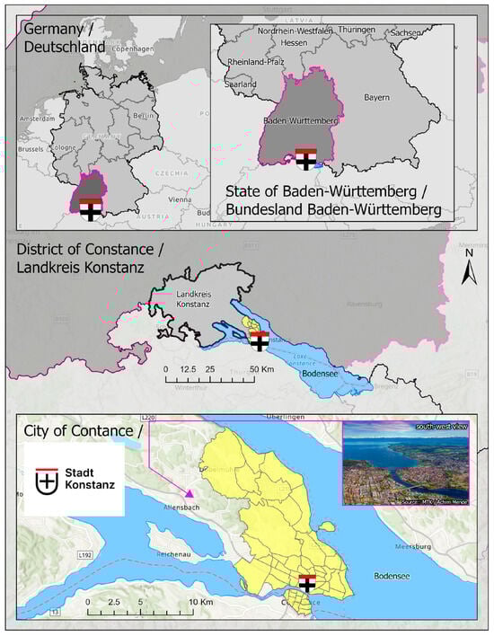
Figure 1.
The location of the City of Constance.
3. Data and Processing Methods
Figure 2 summarises the steps to create the model and the subsequent data processing and analysis. The methodology encompasses data preparation and preprocessing steps aimed at deriving vegetation health indicators, including the leaf area index (LAI), fraction of absorbed photosynthetically active radiation (FAPAR), and various vegetation indices. The process involves generating linear model equations to produce a fine resolution of LAI and FAPAR as proxies for vegetation health. Additionally, forest-based regression and classification models are constructed to generate the vegetation climate model to analyse the relationship between bioclimate indicators and vegetation health.
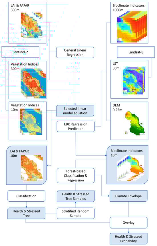
Figure 2.
Flow chart of the methods applied to this study, outlining the steps taken to model, data processing, and the various analyses conducted.
3.1. Data Collection
This study developed vegetation–climate models by integrating spatial data from the C3S Climate Data Store (CDS) and remote sensing data. Given the limitations in data availability, models were parameterised based on the best available data and the local literature. The data obtained from CDS included ten-daily gridded datasets of LAI and FAPAR at a resolution of 300 m for July 2018 as the most current data available at the peak of vegetation’s growing seasons [19] and six variables of bioclimate indicators consists of mean temperature of the warmest quarter (BIO10), mean temperature of the coldest quarter (BIO11), annual temperature range (BIO07), minimum temperature of the coldest month (BIO06), precipitation of the driest month (BIO14), and annual moisture index (MI) in the time frame of 2009–2030. The time frame was chosen as close as possible to the year when this study commenced.
We used Sentinel-2, acquired in July 2018 and July 2022, for multispectral bands at the resolutions of 10 m and 20 m (the bands used are described in Table 1. Sentinel-2 was used because it was freely available for the study area and because it provided many multispectral bands to derive vegetation indices as the indicators for downscaling LAI and FAPAR. A topographic correction (ATCOR) algorithm was used to obtain bottom-of-atmosphere reflectance in a cartographic projection. The Landsat 8 thermal infrared bands from 2012 to 2022 were used to derive land surface temperature at a 30 m resolution. The time frame was chosen as close as possible to the bioclimate indicator time frame. We also used a 0.25 m digital elevation model (DEM) obtained from the State Office for Geoinformation and Land Development of Baden-Württemberg.

Table 1.
Description and equations for vegetation indices.
The vegetation cover was obtained from the WorldCover Land Cover product at 10 m resolution for 2020, as the most recent data available [20]. This dataset was derived from Sentinel-1 C-band Synthetic Aperture Radar (SAR) and Sentinel-2 multispectral bands using the Land Cover Classification System (LCCS) by the Food Agriculture Organization of the United Nations, achieving a global accuracy of 74.4%. We also used the most updated Tree Street Layer 2018 data from Copernicus Land Monitoring Services to identify tree patches in urban areas [21].
3.2. Data Preparation and Preprocessing
This section outlines the preparation and preprocessing steps undertaken on the downloaded data prior to its subsequent analysis. These measures were implemented to standardise the data, ensuring uniformity in both extent and format.
3.2.1. Vegetation Cover
This study focused on urban ecosystems with varying densities and morphological features, particularly urban forests. The vegetation cover was derived from the Copernicus database, utilising land cover data with accuracies of ≥74.4% for ESA WorldCover and ≥85% for Corine Land Cover, which was suitable for this study due to minimal land cover changes in the past two years. The classification involved trees, non-trees, and non-vegetation all over the City of Constance. Tree cover was reclassified based on land cover from the WorldCover Land Cover product, identified as areas dominated by at least 10% tree canopy as tree cover, including urban forests and other trees. Copernicus Tree Street Layer 2018 data were also incorporated to fill the tree’s gaps in settlement areas [21]. Other vegetation types were reclassified as other non-trees, and the rest as non-vegetation. Overall, the trees were distributed in the northern and middle west of the city, along with some parts of the southern and urban areas, comprising various coniferous and broadleaf trees.
3.2.2. Vegetation Indices
Atmospherically corrected and spectrally calibrated Sentinel-2 images were utilised to generate five vegetation indices at 300 m and 10 m resolutions. These indices include the Moisture Stress Index (MSI) for plant water stress, the Normalised Difference Vegetation Index (NDVI) for greenness, the Plant Senescence Reflectance Index (PSRI) for plant senescence, the Red Edge Normalised Difference Vegetation Index (RNDVI) for chlorophyll content, and the Soil-Adjusted Vegetation Index (SAVI) to account for soil brightness in low vegetation cover areas, as explained in Table 1.
The computation was performed at a finer resolution of 10 m to align with the red-edge band acquired in July 2022 and at a coarse resolution of 300 m to match the LAI and FAPAR products of CDS acquired in July 2018. The SAVI index was introduced to reduce soil effects, which identified the variables affecting vegetation index performance, including soil reflectance, vegetation amount, and canopy architecture [22]. The calculation for SAVI included the index’s multiplication factor (1 + L), which maintains the dynamic range. An adjustment factor (L) was decided based on the vegetation densities. An optimal factor L of 0.5 was chosen in the study area to reduce soil noise in the canopy cover because the study area is covered by various vegetation densities [23].
3.2.3. Land Surface Temperature
Landsat 8 TIRs were used to retrieve the land surface temperature (LST) by inverting the radiative transfer according to the equation referred to by Onačillová et al. (2022) from 2012 to 2022 [15]. LST was derived as one of the data points to downscale several coarse bioclimatic indicators from CDS with a 20-year temporal resolution. The time frame was chosen to align the selected bioclimatic indicators between 2009 and 2030. Three distinct LSTs were obtained, each corresponding to a specific bioclimatic indicator. The first LST represents the average LST to downscale BIO11 (the mean temperature of the coldest quarter). The dataset is available as a three-month period dataset, holding the months December to February for each consecutive year. The second LST dataset includes the months June to August to downscale BIO10 (the mean temperature of the warmest quarter). Lastly, the third LST dataset obtained by subtracting the temperatures of the warmest and coldest quarter helped downscale BIO07 (the annual temperature range).
3.3. Vegetation Health Proxies
The proxies were constructed to derive vegetation health using biophysical parameters, specifically LAI and FAPAR, employing an empirical approach coupled with a data-driven method.
3.3.1. Linear Model
An empirical approach was used through linear regression to establish the relationships between the vegetation indices and biophysical variables, specifically for LAI and FAPAR. Vegetation indices are a common indicator of vegetation status or growth model assimilation used to estimate LAI and FAPAR using remote sensing [24]. Five vegetation indices derived from Sentinel-2 in July 2018 were resampled to a coarser resolution of 300 m. The resampled images served as explanatory variables in the linear regression model of LAI and FAPAR from CDS. The relationships between vegetation indices and LAI/FAPAR at 300 m resolution were then used as a reference to develop a generalised linear regression model for estimating LAI and FAPAR at a higher resolution of 10 m.
The equation for LAI and FAPAR calculation at 300 m resolution is derived using the output coefficient (a0 − a4):
LAI300m = a0 + a1 × VI300m (1) + a2 × VI300m (2) + … + an × VI300m (n)
LAI10m at the finer resolution is computed by applying the Equation (1) model, where vegetation indices at 10 m resolution replace the input vegetation indices at 300 m resolution. The following equation is used:
LAI10m = a0 + a1 × VI10m (1) + a2 × VI10m (2) + … + an × VI10m (n)
This study made use of the abovementioned Equation (1) and the most recent available 2018 CDS dataset [25], which were used to calculate the 2022 Equation (2), assuming that there are no significant changes in vegetation cover between the different years, especially for vegetation cover, since there were no major climate-induced events that could have a major impact on the vegetation in the study area.
The model performance was measured using the Akaike Information Criterion (AIC), the corrected Akaike Information Criterion (AICc), multiple R-squared, and adjusted R-squared. AIC considers the model’s complexity useful for comparing models with different explanatory variables, while AICc applies bias correction to AIC for small sample sizes. AIC with a lower value is considered more accurate. Meanwhile, multiple R-squared measures the goodness of fits, with higher values preferable. Adjusted R-squared compensates for the number of variables in the model, where the value is almost always less than multiple R-squared.
The linear model has been used for similar studies to generate the equation to predict the result in higher resolution; for example, utilising Sentinel-2 for land surface temperature production in higher resolution based on Landsat [26] and utilising vegetation indices and CDS bioclimate indicators to predict LAI. The limitation of this empirical relationship is that it can be influenced by external factors that cannot be easily implemented in the model, such as sun–surface–sensor geometry of satellite imagery, crop management practices, and environmental and climatic conditions.
3.3.2. Vegetation Health Classification
The healthy and stressed vegetation classification was conducted using a data-driven method. The threshold for healthy and stressed vegetation types was established, referring to previous studies that examined LAI and FAPAR values for different vegetation types and their statistical characteristics. Healthy vegetation was classified for all pixel values above the first quartile of LAI and FAPAR, while stressed vegetation has mean values equal to or below the minimum reference values (Table 2 and Table 3) of each corresponding vegetation type. The mean values of LAI and FAPAR for several vegetation types in Table 2 and Table 3 show no significant difference between the Visible/Infrared Image Radiometer Suite (VIR) and MODIS (MOD) [27].
Table 2.
The comparison of LAI and FAPAR on several vegetation types [27].
Table 3.
The LAI value of several vegetation types [28].
We produced two vegetation health maps based on LAI and FAPAR data. In the final step, we classified healthy vegetation if either LAI or FAPAR indicated a healthy status. Stressed vegetation was classified when both LAI and FAPAR indicated a stressed condition.
3.4. Vegetation Climate Model
This section encompasses the procedures for downscaling the coarse resolution of climate data to align with municipal levels (Section 3.4.1), constructing the vegetation climate model (Section 3.4.2), and validating the model’s accuracy (Section 3.4.3).
3.4.1. Empirical Bayesian Kriging Regression Prediction
An Empirical Bayesian Kriging (EBK) regression prediction was employed to downscale the bioclimate indicators. It is a geostatistical interpolation method that combines kriging and regression analysis, using an explanatory variable raster to improve interpolation accuracy. This combination of methods yielded more precise predictions than kriging or regression alone. In this process, a digital elevation model (DEM) with a resolution of 0.25 m and Landsat-derived land surface temperature (LST) data with a resolution of 30 m were used as parameters for certain bioclimatic indicators [29]. The summary of parameters for downscaling bioclimate indicators is presented in Table 4.
Table 4.
Parameters used for downscaling bioclimate indicators.
Bioclimate indicators have been studied for years to predict plant-type distribution patterns [12]. The bioclimate indicators used in this study consisted of four variables (BIO11, BIO06, MI, and BIO14) representing winter temperature, moisture balance, dry season precipitation, and summer temperature (BIO10) influencing vegetation distribution. BIO11 represents the mean temperature of the coldest quarter, providing insights into the effects of environmental factors on seasonal distributions. BIO06 indicates the minimum temperature of the coldest month, examining the impact of cold temperature anomalies throughout the year on species distribution. MI (annual moisture index) is calculated by dividing average annual precipitation (RCP) by average annual potential evapotranspiration (PET) and informs about moisture availability for species distribution. BIO14 represents the precipitation of the driest month, analysing the influence of extreme precipitation conditions on the potential species range. BIO10 corresponds to the mean temperature of the warmest quarter, providing information about the effects of environmental factors on seasonal distributions. Lastly, BIO07 (annual temperature range) indicates the difference between the maximum temperature of the warmest month and the minimum temperature of the coldest month, assessing how extreme temperature conditions may affect species distribution.
3.4.2. Forest-Based Classification and Regression
This study utilised a forest-based regression and classification tool adopted by Leo Breiman’s random forest algorithm. This tool was used to create a bioclimate envelope model using finer-generated bioclimate indicators. This algorithm creates an ensemble of decision trees using a known training dataset to predict values in unknown datasets with several explanatory variables. The decision for the final prediction is obtained through a voting scheme to avoid overfitting the model [30]. By examining the characteristics of bioclimate indicators in the train samples of vegetation, this model was employed to generate the bioclimate envelope.
The bioclimatic envelope concept aims to predict the optimal climate conditions for vegetation growth and reproduction. The forest-based regression and classification method investigated the relationship between vegetation and climate conditions. Samples of 300,000 points representing vegetation health status were obtained through stratified random sampling; the model was trained on 90% of the data and tested on the remaining 10% to assess its performance. The explanatory variables in the model were downscaled bioclimatic indicators. The potential distribution range of vegetation types was determined by setting maximum and minimum thresholds for six bioclimatic variables.
Upper and lower limit values for each bioclimatic indicator were identified to assess the potential suitability of climatic conditions for vegetation growth. These values indicated whether the climate conditions were suitable for vegetation to grow. However, the model did not provide the probability of vegetation growing healthy or stressed. The climate envelope was overlaid with the vegetation health status obtained from the linear model of LAI and FAPAR using a raster calculator to derive the probability of vegetation health. This process generated vegetation health probability maps, indicating locations where vegetation will grow in healthy and stressed states.
3.4.3. Model Validation
In this study, model validation aimed to assess the reliability and effectiveness of the derived models by comparing them to reference data. Two validation procedures were conducted. First, the linear model’s performance in estimating LAI and FAPAR was evaluated by comparing the results with those obtained using the SNAP 9.0.0 software commonly used in vegetation-related research. Scatter plots were created to examine the correlation between the two data sets, with SNAP-derived LAI and FAPAR considered suitable for this study due to their focus on urban areas with limited or very dense vegetation. Second, the accuracy of the climate envelope generated through forest-based classification and regression. The result was summarised using a confusion matrix. This matrix compared the predicted vegetation types with actual land cover classifications from Copernicus ESA’s WorldCover dataset. For validation purposes, 5456 samples were randomly generated using a stratified random sampling approach.
4. Results
4.1. Vegetation Health Proxies
Vegetation compositions in the City of Constance exhibit considerable diversity. In this study, we assessed vegetation health by examining satellite-derived biophysical parameters, specifically leaf area index (LAI) and fraction of absorbed photosynthetically active radiation (FAPAR).
4.1.1. Vegetation Indices, LAI, and FAPAR
The LAI and FAPAR products from CDS with 300 m resolution were insufficient for application in urban vegetation studies. Therefore, we used several downscaling methods to generate finer-resolution data, and an empirical approach was used to estimate LAI and FAPAR at a higher resolution. It adapted relationships from general linear regression equations derived from field data collection [24].
Vegetation indices generated from Sentinel-2 at a resolution of 10 m were computed, representing various aspects of vegetation, including the MSI, NDVI, SAVI, PSRI, and RNDVI. These indices were derived from specific bands commonly associated with capturing vegetation characteristics based on their reflectance properties [31]. NDVI and SAVI showed strong correlations with leaf area index (LAI) and fraction of absorbed photosynthetically active radiation (FAPAR), reaching 0.71 and 0.74, respectively. RNDVI exhibited slightly lower correlations with LAI and FAPAR, at 0.69 and 0.70, respectively. In contrast, MSI and PSRI showed negative correlations, with MSI having a correlation of 0.66 for LAI and 0.67 for FAPAR, while PSRI had the lowest correlation values, with 0.52 for LAI and 0.50 for FAPAR.
4.1.2. Linear Model
Linear regression equations were developed to predict LAI and FAPAR using combinations of these vegetation indices (Table 5 and Table 6). The most optimal regression equations have high R-squared values and low AIC values. In this study, explanatory regression was used to investigate the consistency of vegetation indices in predicting LAI and FAPAR. NDVI, SAVI, and PSRI showed significant and stable influences on LAI and FAPAR, with NDVI and SAVI demonstrating 100% positive relationships, while PSRI showed 91.67% positive and 8.33% negative relationships. The NDVI, PSRI, SAVI, and PSRI combinations produced the most optimal regression equations with high R-squared and low AIC values.
Table 5.
The LAI equations were derived from general linear regression.
Table 6.
The FAPAR equations were derived from general linear regression.
Considering the study area’s characteristics with varied vegetation cover and tree cover, the NDVI and PSRI equations were chosen. However, if the study area is primarily covered by low vegetation, SAVI is recommended for use. The vegetation index of SAVI attempts to minimise the influence of soil brightness in areas of low vegetation cover using a soil brightness correction factor.
The mathematical equations derived from 2018 data were used to estimate LAI and FAPAR in 2022, assuming no significant landscape changes in the City of Constance within the four years. The coefficient determination (R-squared) for the NDVI and PSRI equations was approximately 0.78, indicating the model’s accuracy based on CDS data as a reference.
The equations used for generating LAI and FAPAR were
LAI10m = 3.79 × NDVI + 1.39 × PSRI − 0.82
FAPAR10m = 0.88 × NDVI + 0.41 × PSRI + 0.04
The comparison of the originally downloaded LAI and FAPAR from CDS and the generated linear model LAI and FAPAR is shown in Figure 3.
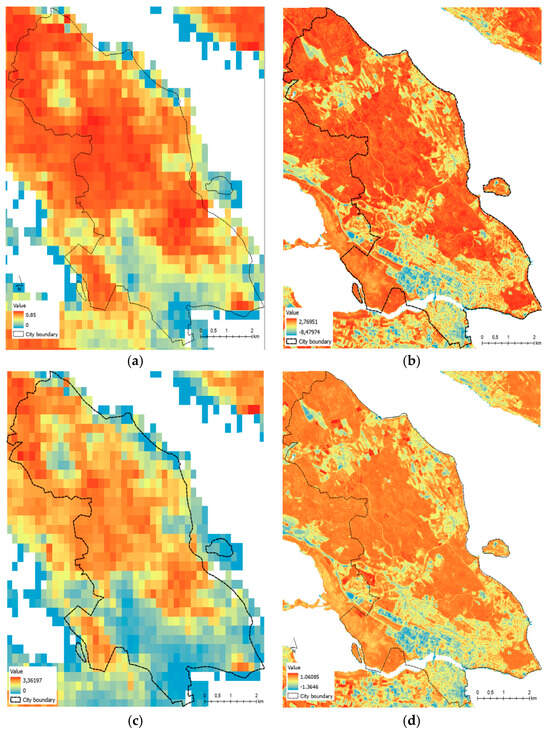
Figure 3.
The comparison of LAI/FAPAR: (a) original downloaded LAI from CDS; (b) linear model LAI; (c) original downloaded FAPAR from CDS; (d) linear model FAPAR.
The performance of the linear model in estimating LAI and FAPAR was compared to the SNAP software results for the same year. The R-squared values for the linear model and SNAP-derived LAI were 0.65 and 0.92 for FAPAR. SNAP-derived LAI tended to produce higher values than the linear model, which is consistent with previous studies [32,33]. However, for the study area’s vegetation, which primarily consists of tree-covered forest and urban areas, both linear models and SNAP-derived LAI and FAPAR are feasible.
4.1.3. Vegetation Health Classification
The classification value for vegetation health status is presented in Table 7, and the map of vegetation health classification is shown in Figure 4. Similar studies using different datasets to estimate LAI have demonstrated comparable values for corresponding types of vegetation cover. The classification outcomes indicate the presence of negative LAI and FAPAR values across all vegetation types. Therefore, to understand the causes, we overlayed the results with land cover data. The overlay analysis showed that these areas were frequently found at mixed and misclassified pixels.
Table 7.
The range of LAI and FAPAR values of the vegetation cover in the study area.
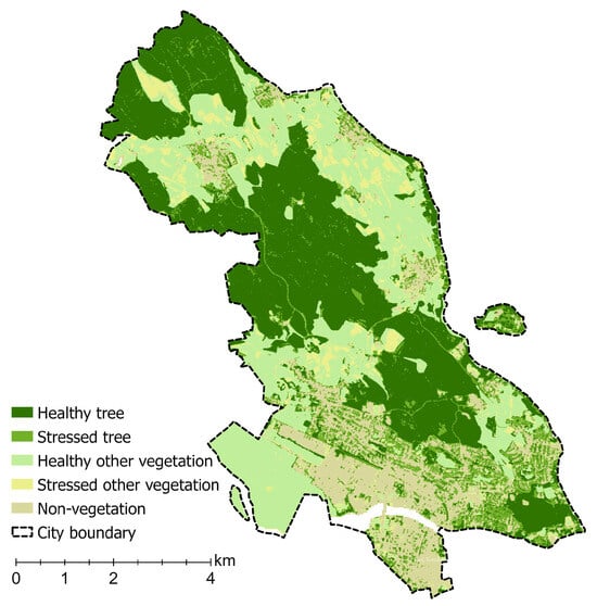
Figure 4.
The map of vegetation health status.
Healthy trees were predominantly found in forested areas with a dense concentration of trees, especially in urban forests. Stressed trees were commonly found in street areas and close to built-up regions, with dead branches as indicators of stress symptoms. Warmer temperatures can enhance the carbon assimilation rate, leading to enlarged canopy cover in trees. However, water deficits can cause defoliation, especially in urban areas where rising temperatures may result in early summer defoliation.
While stressed trees in urban areas may face challenges, their presence is crucial in mitigating urban heat and creating a cooling effect. Understanding the correlation between vegetation and climate is essential, especially in urban areas, as urban vegetation can mitigate the negative impacts of climate change while being vulnerable to increasing temperatures and drought events.
In other vegetations, the difference between healthy and stressed vegetation is based on the amount of vegetation cover. Stressed vegetation was predominantly found in grasslands with high soil reflectance and unplanted cropland areas, even during peak summer when satellite images were acquired (July).
4.2. Vegetation and Climate Relations
Various bioclimate parameters were utilised across different vegetation types to identify optimal climate conditions conducive to the healthy growth of each vegetation type. This investigation aimed to establish the correlation between local-scale climate conditions and vegetation.
4.2.1. Vegetation Climate Model
The vegetation climate model identifies optimal climatic conditions for vegetation growth and adaptation to extreme climate changes, as shown in Figure 5a. It defines climatic boundaries for trees and other vegetation in the City of Constance, assuming they will not grow if local climate variables exceed those defining its envelope. The range value of the bioclimate envelope is shown in Table 8.
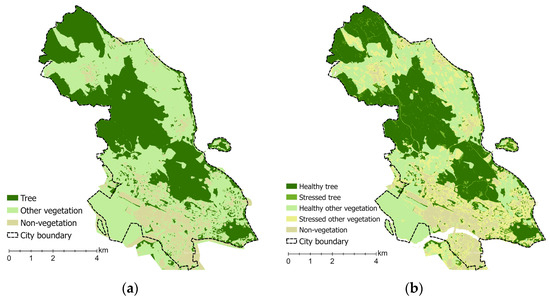
Figure 5.
The probability of location for vegetation generated from random forest regression and classification: (a) vegetation can grow both healthy and stressed; (b) vegetation can grow healthy and stressed.
Table 8.
The range of bioclimate indicators of the vegetation cover in the study area.
This model predicts the natural location range of vegetation to grow in healthy and stressed conditions. It assumes vegetation can grow well within its predicted natural conditions. However, specific adjustments may be needed outside of these locations. The model was combined with LAI- and FAPAR-derived vegetation health status to determine the probability of healthy and stressed vegetation, as shown in Figure 5b. The model achieved high r-squared values for training (0.97) and validation (0.84) data, utilising six downscaled bioclimatic indicators as explanatory variables.
The bioclimate envelope model outlines the potential occurrence range for each vegetation type based on six variables’ maximum and minimum values. Minimum precipitation during the driest month (BIO14) represents the maximum drought vegetation can withstand, with trees and other vegetation requiring 0.02 mm. The upper limit of precipitation indicates the drought level inducing dormancy. Trees show better acclimatisation ability under changing climates (higher BIO14) than other vegetation types. The mean temperature during the warmest quarter (BIO10) is relatively similar among trees and other vegetation, with trees having a slightly wider range. Warmer temperatures within an optimal range stimulate photosynthetic activities. The lower limit represents the minimum temperature requirement for growth. The annual moisture index is useful for predicting vegetation types and forest areas. The minimum temperature of the coldest month (BIO06) can help identify anomalies in cold temperatures that may impact vegetation, while the annual temperature range (BIO07) indicates the potential effects of extreme temperatures on vegetation. BIO10 and BIO14 indicate the ability of that vegetation to withstand the average warmest period and the driest month.
4.2.2. Model Validation
The climate envelope model was validated by comparing it with existing vegetation from ESA WorldCover 2020, resulting in an overall accuracy of 86.7%. The result was summarised in the confusion matrix, as shown in Table 9.
Table 9.
Confusion matrix of the climate envelope and ESA WorldCover 2020.
The kappa value, representing the level of agreement beyond chance, was 0.74, which is slightly lower than the overall accuracy. The model utilised a bioclimatic envelope concept, associating various climate aspects with species occurrences to estimate suitable conditions for vegetation. Producer accuracy for vegetation types shown in the climate envelope and ESA WorldCover ranged from 70.1% to 75.7%, indicating the percentage of reference pixels classified correctly. User accuracy varied for trees and other vegetation: 83.1% for other vegetation, 93.4% for trees, and 98.6% for non-vegetation.
4.3. Integrate Workflows into a Toolbox
This study utilised a range of global climatic data from CDS and other resources for climate monitoring, integrating different data sources to improve the results at the municipal level. Multiple processes of data acquisition and processing were employed in this study. The main process involved sequences of geoprocessing performed using model builders from ArcGIS Pro combined with a Python notebook. The model builder is an automated tool that connects data and available tools in ArcGIS Pro to execute workflows efficiently.
We created a toolbox called vegetation health, containing four toolsets representing different geoprocessing steps: vegetation indices (Figure 6), biophysical processors (Figure 7), vegetation health (Figure 8), downscale climate indicators (Figure 9a), and climate envelopes (Figure 9b).
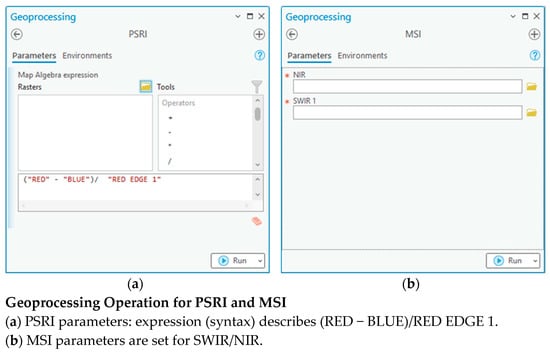
Figure 6.
Vegetation indices toolset consists of (a) PSRI and (b) MSI.
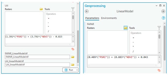
Figure 7.
Biophysical processor toolset to produce respective linear models of LAI and FAPAR in finer resolution.
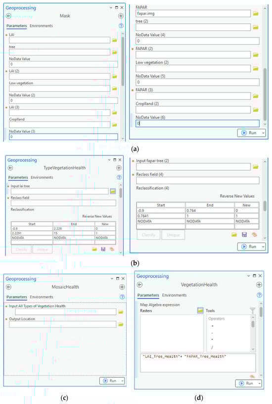
Figure 8.
Vegetation health toolset consists of (a) mask tool for masking each type of vegetation, (b) TypeVegetationHealth tool for classifying healthy and stressed vegetation based on LAI and FAPAR, (c) VegetationHealth for combining vegetation health based on LAI and FAPAR, and (d) MosaicHealth for combining all types of vegetation health.
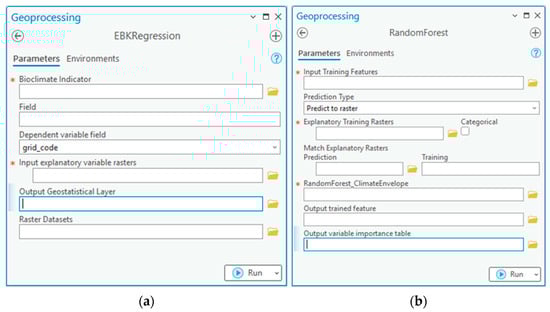
Figure 9.
Downscaled bioclimate indicators and climate envelope toolset consists of (a) EBKRegression tool for downscaling bioclimate indicators and (b) RandomForest for generating climate envelope.
The biophysical processor toolset generated LAI and FAPAR using a model builder with a raster calculator and equations derived from general linear regression. The chosen vegetation indices (NDVI and PSRI) better predicted LAI and FAPAR than others.
The vegetation health toolset consisted of four model builders to classify vegetation health status based on LAI and FAPAR values. The process involved separating each vegetation type, identifying their health status, combining all types into a single map, and classifying vegetation health using LAI and FAPAR.
The downscale climate indicators toolset downscaled bioclimate indicators using EBK regression prediction with coarse and fine resolution rasters as explanatory variables, producing bioclimate indicators in finer resolution. The climate envelope toolset executed forest-based classification and regression, building a vegetation climate model called the climate envelope. It used vegetation-type point samples and bioclimate indicators in finer resolution as explanatory variables, providing a vegetation map showing the probability of healthy and stressed vegetation growth.
5. Discussion
5.1. Consideration of Approach and Interpretation of Vegetation Climate Model
Climate factors play a crucial role in influencing vegetation greenness, which is one of the key indicators of vegetation health. We used greenness and senescence indexes for assessing vegetation health in this study. The vegetation response to climate variation and adaptability is complex yet challenging to accurately simulate. Most studies assumed that vegetation has a fixed response pattern to climate change. Despite its limitations, the vegetation–climate relations model is important to understand how it impacts the environment.
Understanding how vegetation responds to local weather changes is crucial in microclimate. Microclimate refers to localised variations in heat and water moisture levels near the earth’s surface, leading to temperature and humidity differences compared to the surrounding areas. This local atmospheric condition can be influenced by a range of factors, such as energy absorption, shading, and wind speeds, which either trap or remove heat and moisture. The variations surrounding vegetation could potentially influence vegetation health, with healthier vegetation located near denser vegetation and stressed vegetation in isolated areas. Vegetation growing close to dense vegetation benefits from shading and moisture. In contrast, isolated vegetation surrounded by non-vegetation areas tends to experience more stress. It was shown in the vegetation health classification from the linear models of LAI and FAPAR that stressed vegetation is often found farther away from other vegetated areas.
This study combined the big data platform and local data to provide an adequate municipal-level model on a finer resolution scale. We performed multiple processes to downscale existing coarse data using remote sensing and local data. Statistical downscaling methods were employed, representing a flexible and straightforward approach to enhance the data of coarse resolution. Notably, though our models can be used for monitoring vegetation health, they cannot thoroughly describe the relationship between the climate and vegetation, especially for non-trees, which consist of various types of vegetation, such as wetland-sensitive biomes to temperature and with the highest interannual variability.
The climate envelope model was valuable for assessing suitable tree and other vegetation locations based on current climate conditions. For example, areas close to parks can be cooler during daylight hours compared to rooftops due to the cooling effect of transpiration. Sparse foliage areas exhibit higher temperatures due to less evaporation than areas covered by dense foliage. Besides the climate factors, elevated atmospheric CO2 concentration, varying nitrogen deposition rates, land use, and other anthropic factors could also influence vegetation health, which may bring a greater potential for vegetation change due to the more complex factors. We have not considered these additional factors in the model in this study. Further, we can explore the more complex social-ecological systems by inputting more natural and anthropogenic variables and coupling them with specific physical processes based on advanced modelling to better understand the complex relationship between vegetation and environments.
5.2. Additional Management Considerations
We produced linear model equations and a vegetation–climate model that exhibits potential applicability to municipalities sharing similarities with the City of Constance. This contribution extends beyond the specific study area, offering a transferable framework for regions exhibiting comparable characteristics. Additionally, the incorporation of a toolbox into our methodology serves as an effective means to introduce these models to municipal stakeholders lacking expertise in spatial data analysis. This approach enhances accessibility, facilitating wider utilisation and implementation in diverse municipal contexts.
Vegetation climate models at the municipal level offer valuable contributions to the conservation and management of urban ecosystems. The bioclimate envelope models derived from this study have numerous sources of uncertainty, including method choices, data used, and climate dynamics. Despite its limitations, the analysis provides useful tools for assessing climate impacts on urban vegetation, especially the information on the potential location for vegetation growth. This information empowers decision-makers to explore existing ecosystems within these environments, understand their function, and gather essential information for adaptation measures and planning. Integrating non-climatic factors and adaptive capacity information enhances the potential for conducting comprehensive ecological climate change vulnerability assessment in urban environments, presenting a crucial step towards effective urban ecosystem conservation.
6. Conclusions
This study proposes utilising Copernicus data, which provide various climatic and environmental data and information in various resolutions for municipal-level studies. The entire process was executed using the model builder functionality within ArcGIS, enabling conversion into toolboxes along with a sequence of Python scripts. We used downscaled methodologies to improve the resolution of data LAI, FAPAR, and bioclimate indicators by investigating the best and most reliable method for each dataset based on its characteristics and combining data from satellite images and local data. This method was used, including general linear regression and EBK regression and prediction, which are simple and fast statistical techniques to derive local-scale data. The final results were climatic envelopes to predict the probability location for vegetation to grow healthy and stressed based on the bioclimate indicators. This overall approach is especially useful for characterising the optimum location for vegetation types in an urban environment in response to climate conditions.
Author Contributions
Conceptualization, F.K. and C.S.; Methodology, F.K.; Software, F.K. and C.S.; Validation, F.K. and C.S.; Data curation, F.K. and C.S.; Writing—original draft, F.K. and C.S.; Writing—review & editing, F.K. and C.S.; Review, M.M. and V.S.; Visualization, F.K. and C.S.; Supervision, V.S; Project administration, C.S. and M.M; Funding acquisition, V.S., M.M. and C.S. All authors have read and agreed to the published version of the manuscript.
Funding
This research was partially supported by the project CoKLIMAx, grant number 50EW2103A-D, funded by the German Aerospace Center (DLR) and Federal Ministry of Transport and Digital Infrastructure (BMDV).
Data Availability Statement
The data were retrieved from (1) COPERNICUS C3S Climate Data Store, (2) CODE-DE, (3) NASA Open Data Portal, and (4) local data provided by the City of Constance/ Stadt Konstanz am Bodensee.
Acknowledgments
The publication is based on a master thesis at Stuttgart University of Applied Sciences (HFT) and the University of Stuttgart, Institute of Engineering Geodesy (IIGS), that was co. supervised by C. Sebald. The support of M. Hahn. from the Stuttgart University of Applied Sciences (HFT) is gratefully acknowledged. The authors would also like to thank the editors and the reviewers for their help and suggestions.
Conflicts of Interest
The authors declare no conflicts of interest.
References
- Kabisch, N.; Korn, H.; Stadler, J.; Bonn, A. Nature-Based Solutions to Climate Change Adaptation in Urban Areas, Theory and Practice of Urban Sustainability; Springer: Cham, Switzerland, 2017; ISBN 978-3-319-53750-4. [Google Scholar]
- European Environment Agency. Extreme Weather: Floods, Droughts and Heatwaves. Available online: https://www.eea.europa.eu/en/topics/in-depth/extreme-weather-floods-droughts-and-heatwaves (accessed on 30 January 2024).
- European Environment Agency. Urban Adaptation to Climate Change in Europe 2016—Transforming Cities in a Changing Climate; Publication Office of the European Union: Luxembourg, 2016; ISBN 978-92-9213-742-7. [Google Scholar]
- Gamble, J.L.; Balbus, J.; Berger, M.; Bouye, K.; Campbell, V.; Chief, K.; Conlon, K.; Crimmins, A.; Flanagan, B.; Gonzalez-Maddux, C.; et al. The Impacts of Climate Change on Human Health in the United States: A Scientific Assessment; U.S. Global Change Impact Program: Washington, DC, USA, 2016. [CrossRef]
- European Environment Agency. Urban Adaptation in Europe: How Cities and Towns Respond to Climate Change; Publication Office of the European Union: Luxembourg, 2020; ISBN 978-92-9480-270-5. [Google Scholar]
- Copernicus. Copernicus History Overview. Available online: https://defence-industry-space.ec.europa.eu/system/files/2022-03/Copernicus%20History%20EN.pdf (accessed on 31 January 2024).
- Bühler, M.M.; Sebald, C.; Rechid, D.; Baier, E.; Michalski, A.; Rothstein, B.; Nübel, K.; Metzner, M.; Schwieger, V.; Harrs, J.A.; et al. Application of Copernicus Data for Climate-Relevant Urban Planning Using the Example of Water, Heat, and Vegetation. Remote Sens. 2021, 13, 3634. [Google Scholar] [CrossRef]
- Zarco-Tejada, P.; Sepulcre-Cantó, G. Remote Sensing of Vegetation Biophysical Parameters for Detecting Stress Condition and Land Cover Changes. Estud. Zona No Saturada Suelo 2007, VIII, 37–44. [Google Scholar]
- Wu, H.; Li, Z.L. Scale Issues in Remote Sensing: A Review on Analysis, Processing and Modeling. Sensors 2009, 9, 1768–1793. [Google Scholar] [CrossRef]
- Chen, Z.; Liu, H.; Xu, C.; Wu, X.; Liang, B.; Cao, J.; Chen, D. Modeling Vegetation Greenness and Its Climate Sensitivity with Deep-Learning Technology. Ecol. Evol. 2021, 11, 7335–7345. [Google Scholar] [CrossRef] [PubMed]
- Heikkinen, R.K.; Luoto, M.; Araújo, M.B.; Virkkala, R.; Thuiller, W.; Sykes, M.T. Methods and Uncertainties in Bioclimatic Envelope Modelling under Climate Change. Prog. Phys. Geogr. 2006, 30, 751–777. [Google Scholar] [CrossRef]
- Box, E.O.; Crumpacker, D.W.; Hardin, E.D. A Climatic Model for Location of Plant Species in Florida, U.S.A. J. Biogeogr. 1993, 20, 629. [Google Scholar] [CrossRef]
- Notaro, M.; Mauss, A.; Williams, J.W.; Williams, J.W. Projected Vegetation Changes for the American Southwest: Combined Dynamic Modeling and Bioclimatic-Envelope Approach. Ecol. Appl. 2012, 22, 1365–1388. [Google Scholar] [CrossRef] [PubMed]
- Magness, D.R.; Morton, J.M. Using Climate Envelope Models to Identify Potential Ecological Trajectories on the Kenai Peninsula, Alaska. PLoS ONE 2018, 13, e0208883. [Google Scholar] [CrossRef]
- Onačillová, K.; Gallay, M.; Paluba, D.; Péliová, A.; Tokarčík, O.; Laubertová, D. Combining Landsat 8 and Sentinel-2 Data in Google Earth Engine to Derive Higher Resolution Land Surface Temperature Maps in Urban Environment. Remote Sens. 2022, 14, 4076. [Google Scholar] [CrossRef]
- Rösch, M. Prehistoric Land Use as Recorded in a Lake-Shore Core at Lake. Veg. Hist. Archaeobot 1993, 2, 213–232. [Google Scholar] [CrossRef]
- Lechterbeck, J.; Rösch, M. Böhringer See, Western Lake Constance (Germany): An 8500 Year Record of Vegetation Change. Grana 2021, 60, 119–131. [Google Scholar] [CrossRef]
- Heugel, A.; Chilla, T. Lake Constance; ESPON EGTC: Luxembourg, 2020; ISBN 978-2-919816-26-2. [Google Scholar]
- Weiss, J.L.; Gutzler, D.S.; Coonrod, J.E.A.; Dahm, C.N. Long-Term Vegetation Monitoring with NDVI in a Diverse Semi-Arid Setting, Central New Mexico, USA. J. Arid. Environ. 2004, 58, 249–272. [Google Scholar] [CrossRef]
- Zanaga, D.; Van De Kerchove, R.; De Keersmaecker, W.; Souverijins, N.; Brockmann, C.; Quast, R.; Wevers, J.; Grosu, A.; Paccini, A.; Vergnaud, S.; et al. ESA WorldCover 10 m 2020 V100. Available online: https://doi.org/10.5281/zenodo.5571936 (accessed on 19 August 2022).
- Urban Atlas Street Tree Layer 2018. Available online: https://doi.org/10.2909/205691b3-7ae9-41dd-abf1-1fbf60d72c8c (accessed on 24 September 2022).
- Rondeaux, G.; Steven, M.; Baret, F. Optimization of Soil-Adjusted Vegetation Indices. Remote Sens. Environ. 1996, 55, 55–95. [Google Scholar] [CrossRef]
- Huete, A.R. A Soil-Adjusted Vegetation Index (SAVI) 295. Remote Sens. Environ. 1988, 25, 295–309. [Google Scholar] [CrossRef]
- Bajocco, S.; Ginaldi, F.; Savian, F.; Morelli, D.; Scaglione, M.; Fanchini, D.; Raparelli, E.; Bregaglio, S.U.M. On the Use of NDVI to Estimate LAI in Field Crops: Implementing a Conversion Equation Library. Remote Sens. 2022, 14, 3554. [Google Scholar] [CrossRef]
- Copernicus Climate Change Service (C3S); Climate Data Store (CDS); Copernicus Climate Change Service. Leaf Area Index and Fraction Absorbed of Photosynthetically Active Radiation 10-Daily Gridded Data from 1981 to Present. 2018. Available online: https://doi.org/10.24381/cds.7e59b01a (accessed on 20 June 2022).
- Bonafoni, S.; Anniballe, R.; Gioli, B.; Toscano, P. Downscaling Landsat Land Surface Temperature over the Urban Area of Florence. Eur. J. Remote Sens. 2016, 49, 553–569. [Google Scholar] [CrossRef]
- Yan, K.; Chen, C.; Xu, B.; Knyazikhin, Y.; Myneni, R. VIIRS Leaf Area Index (LAI) and Fraction of Photosynthetically Active Radiation Absorbed by Vegetation (FPAR) Product Algorithm Theoretical Basis Document (ATBD). Available online: https://lpdaac.usgs.gov/documents/125/VNP15_ATBD.pdf (accessed on 10 October 2022).
- Buermann, W.; Wang, Y.; Dong, J.; Zhou, L.; Zeng, X.; Dickinson, R.E.; Potter, C.S.; Myneni, R.B. Analysis of a Multiyear Global Vegetation Leaf Area Index Data Set. J. Geophys. Res. Atmos. 2002, 107, ACL 14-1–ACL 14-16. [Google Scholar] [CrossRef]
- Daly, C.; Halbleib, M.; Smith, J.I.; Gibson, W.P.; Doggett, M.K.; Taylor, G.H.; Curtis, J.; Pasteris, P.P. Physiographically Sensitive Mapping of Climatological Temperature and Precipitation across the Conterminous United States. Int. J. Climatol. 2008, 28, 2031–2064. [Google Scholar] [CrossRef]
- Breiman, L. Random Forests. In Machine Learning; Springer Nature: Berkeley, CA, USA, 2001; Volume 45, pp. 5–32. [Google Scholar] [CrossRef]
- Cârlan, I.; Mihai, B.A.; Nistor, C.; Große-Stoltenberg, A. Identifying Urban Vegetation Stress Factors Based on Open Access Remote Sensing Imagery and Field Observations. Ecol. Inform. 2020, 55, 101032. [Google Scholar] [CrossRef]
- Zbigniew, B.; Dąbrowska-Zielińska, K.; Gurdak, R.; Niro, F.; Bartold, M.; Grzybowski, P. Validation of LAI Biphysical Product Derived from Sentinel-2 and Proba-V Images for Witner in Western Poland. Geoinf. Issues 2017, 9, 15–26. [Google Scholar]
- Kamenova, I.; Dimitrov, P. Evaluation of Sentinel-2 Vegetation Indices for Prediction of LAI, FAPAR and FCover of Winter Wheat in Bulgaria. Eur. J. Remote Sens. 2021, 54, 89–108. [Google Scholar] [CrossRef]
Disclaimer/Publisher’s Note: The statements, opinions and data contained in all publications are solely those of the individual author(s) and contributor(s) and not of MDPI and/or the editor(s). MDPI and/or the editor(s) disclaim responsibility for any injury to people or property resulting from any ideas, methods, instructions or products referred to in the content. |
© 2024 by the authors. Licensee MDPI, Basel, Switzerland. This article is an open access article distributed under the terms and conditions of the Creative Commons Attribution (CC BY) license (https://creativecommons.org/licenses/by/4.0/).