Abstract
Passive location based on TDOA (time difference of arrival) and FDOA (frequency difference of arrival) is the mainstream method for target localization. This paper proposes a fast time–frequency difference positioning method to address issues such as low accuracy, large computational resource utilization, and limited suitability for real-time signal processing in the conventional CAF (cross-ambiguity function)-based approach, aiming to complete the processing of the target radiation source to obtain the target parameters within a short timeframe. In the mixing product operation step of the CAF, a frequency-domain approach replaces the time-domain convolution operation in PW-ZFFT (pre-weighted Zoom-FFT) to reduce the computational load of the CAF. Additionally, a quadratic surface fitting method is used to enhance the accuracy of TDOA and FDOA. The localization solution is obtained using Newton’s method, which can provide more accurate results compared to analytical methods. Next, a signal processing platform is designed with FPGA (field-programmable gate array) and multi-core DSP (digital signal processor), and works by dividing and mapping the algorithm functional modules according to the hardware’s characteristics. We analyze the architectural advantages of multi-core DSP and design methods to improve program performance, such as EDMA transfer optimization, inline function optimization, and cache optimization. Finally, this paper constructs simulation tests in typical positioning scenarios and compares them to hardware measurement results, thus confirming the correctness and real-time capability of the program.
1. Introduction
According to the different sources of observation signals, target detection technology is categorized into active detection technology, which involves the active emission of signals, and passive detection technology, which relies on the passive capture of signals emitted by the target source. Passive detection technology is commonly referred to as an external radiation source radar. The satellite platform detects and processes signals from non-cooperative radiation sources, extracting the location parameters of the radiation source from the received signals. Compared with an active radar, a passive radar exhibits enhanced concealment and safety features [1,2,3]. Passive detection technology has continuously evolved with respect to real-time performance, accuracy, and detection range. The realm of passive detection has given rise to numerous positioning systems and technology types being developed, each offering complementary advantages. One of the most commonly utilized methods is the joint time–frequency difference localization technology, which utilizes intercepted signals emitted by target radiation sources to acquire time difference of arrival (TDOA) and frequency difference of arrival (FDOA) information, enabling precise target location. This location system, characterized by minimal system equipment, extended range, and high concealment, is widely employed in UAV reconnaissance, satellite navigation, and various other fields. Leveraging these advantages, time–frequency difference localization has become a focal point of research in passive detection technology [4].
The effectiveness of joint time–frequency difference localization relies on the accuracy of estimating parameters such as time difference and Doppler frequency difference [5]. Typically, a method employing the cross-ambiguity function (CAF) is utilized for the joint estimation of time difference and frequency difference [6,7]. The cross-ambiguity function can be viewed as a two-dimensional correlation between the time difference and the Doppler frequency difference [8].
Considerable research has been conducted on the localization of target sources using time difference of arrival (TDOA) and frequency difference of arrival (FDOA). In [9], the optimal interpolation factors method was employed to reduce the computational load of mutual fuzzy functions. The work in [10] introduced an algorithm based on the higher-order statistics cross-ambiguity function (CAF-HOS) to reduce the unknown noise correlation effect. Addressing the issue of CAF performance degradation due to time compression from relative target motion, the authors of [11] investigated short-time CAF coherence. In [12], several weighted least-squares methods were employed to obtain the target location without requiring an initial solution. The work in [13] introduced the constrained weighted least squares (CWLS) algorithm for solving target source positioning and velocity. Both these methods can approach the Cramér–Rao lower bound before the threshold effect occurs, demonstrating enhanced positioning performance at high signal-to-noise ratios. The authors of [14] introduced the use of the total least squares (TLS) method for target localization; however, the accuracy of this method falls short of reaching the Cramér–Rao lower bound. In [15,16], time–frequency difference estimation was explored in the contexts of orthogonal frequency division multiplexing (OFDM) signals and linear frequency modulation (LFM) signals. However, these methods are tailored to signals in specific modes, lacking universality. To address the limited FDOA estimation performance of frequency-hopping signals, the authors of [17] proposed a coherent accumulation method, demonstrating superior FDOA estimation accuracy. In comparison to the existing research, this paper makes the following key contributions:
- We improved the PW-ZFFT algorithm. In the process of calculating the mixing product, the time-domain convolution operation of the signal was replaced by frequency-domain multiplication to achieve a fast calculation of cross-ambiguity functions. For long signals, the frequency-domain method can save more calculations, which is especially important for real-time signal processing.
- To balance the computational efficiency and accuracy of the joint time–frequency difference estimation algorithm, we investigated and adopted the quadratic surface fitting method. This method reduces errors caused by numerical discontinuities near the peak of the cross-ambiguity function without significantly increasing the computational load, thus achieving high precision and rapid estimation of time–frequency differences.
- We constructed a heterogeneous signal processing platform based on FPGA and multi-core DSP for implementing the time–frequency difference localization method. By allocating algorithms rationally on this platform and fully utilizing its architectural advantages, we achieved both software and hardware design implementation for joint time–frequency difference localization.
- We proposed a development optimization method based on multi-core DSP, aimed at enhancing program performance and the real-time nature of data processing. This includes EDMA optimization, cache optimization, and inline functions. Through these optimization strategies, we were able to utilize the resources of the DSP multi-core system more effectively, thus enhancing the real-time processing capability of the time–frequency difference localization algorithm.
The rest of this paper is organized as follows: Section 2 introduces the principle of time–frequency difference localization, constructs a joint TDOA/FDOA localization model, and summarizes the improved cross-ambiguity function algorithm and related works in localization solution computation. In Section 3, we construct a signal processing platform for joint time–frequency difference localization, transplant the localization algorithm onto a hardware platform for real-time processing, detail the structure of the hardware platform, and outline the specific implementation methods of each algorithm module. Finally, based on the characteristics of the processor, we provide a development optimization method based on multi-core DSP to improve the real-time nature of signal processing. Section 4 presents a comparison of hardware and simulation localization results in typical localization scenarios, verifying the accuracy and real-time performance of the time–frequency difference joint localization processing platform. Lastly, Section 5 concludes this paper.
2. Related Works
Related works of the passive location theory and localization algorithm are introduced in this section.
There are many passive positioning systems, including one-point positioning, dynamic positioning, cross positioning, etc. Different positioning systems should be selected based on the relative motion status between the radiation source and the positioning station, the number of positioning stations, and other specific characteristics. Parameters that usually need to be measured include received signal strength (RSS), direction of arrival (DOA), time of arrival (TOA), time difference of arrival (TDOA), doppler frequency and doppler frequency change rate, etc. Positioning methods based on a single parameter have many shortcomings in practical applications. Hybrid positioning improves positioning performance by measuring multiple parameters and is simultaneously used to achieve complementary effects. The study of [18] proposes an RSS/TDOA hybrid positioning algorithm based on wireless sensor networks, which achieves high accuracy and convergence speed. Study [19] considers the impact of multipath noise on positioning performance, and proposes a high-resolution estimation technique to implement DOA/TOA positioning. In low signal-to-noise ratio scenarios, estimating the spatial position of the target source performs better than the multipath fingerprinting scheme. The DOA/TDOA joint positioning proposed in the study by [20] solves the limitations of traditional positioning methods when the range of the signal source is unknown, and at the same time improves the accuracy and applicability of near-field and far-field positioning.
The estimation of the target position often requires complex calculations, which generally require processing processes such as signal interception, signal sorting, and signal pairing. However, there are also technologies that use compressed sensing, deep neural networks, etc., to directly perform positioning, which greatly reduces the computational complexity and processing time. Study [21] proposes a precise indoor positioning system based on RSS, which uses the compressed sensing theory to recover sparse signals from a small number of noisy measurements. The system includes two steps—rough positioning and fine positioning, the cluster in which a node is located is first detected by comparing the received signal strengths of multiple clusters—and then the compressed sensing theory is used to further refine the position estimate. Study [22] proposes an improved recurrent neural network (RNN) method for passive signal source localization. Through spatial partitioning, a cost function is designed to convert the positioning of the transmitter into the output of a modified recurrent neural network. These neural networks are both chaotic and stable in terms of convergence.
3. Passive Localization System
This section will elucidate the principles of time–frequency difference positioning and build the echo model, detailing the estimation methods for TDOA and FDOA, as well as the positioning solution methods. Firstly, the principle of time–frequency difference positioning is summarized in Section 3.1. Then, in Section 3.2, the cross-ambiguity function is introduced. The improved PW-ZFFT algorithm is utilized for the rapid computation of the cross-ambiguity function, obtaining coarse estimates of the time–frequency differences. Section 3.3 discusses the method of quadratic surface fitting to obtain precise estimates of time–frequency differences. In Section 3.4, we build a set of positioning equations and solve these nonlinear equations using Newton’s method, thus acquiring the position information of the source.
3.1. Time–Frequency Difference Location Theory
The time–frequency difference-based positioning principle relies on the distance difference between multiple receiving stations and the target source, leading to varying signal arrival times at each station, thereby resulting in a time difference of arrival. Additionally, the speed of multiple satellite-receiving stations relative to the target source differs, causing a frequency difference in the signals received at each station due to the Doppler effect [23,24,25]. By intercepting the signals emitted by the target source and performing analysis and processing, the time difference and frequency difference of the signals arriving at multiple receiving stations can be measured. The time difference of arrival determines an iso-time-difference hyperbolic surface, and the frequency difference yields an iso-frequency-difference surface. Combined with the Earth’s surface equation, they enable the determination of the target source’s location [26]. The key to joint time–frequency difference positioning is the estimation of time delay and Doppler frequency difference. The accuracy of parameter estimation directly affects the accuracy of positioning.
3.2. TDOA and FDOA Estimation
3.2.1. Cross-Ambiguity Function
The CAF method is employed for joint time–frequency difference estimation [27]. This involves initially pre-delaying one of the two signals, and then conjugating and multiplying both signals to generate a mixing product signal. By adjusting the length of the pre-delay τ, multiple mixing product signals are combined to form a mixing product matrix. A Fourier transform is then performed on the frequency difference dimension of this mixing product matrix, resulting in the spectrum of the mixed product, which is the CAF.
Assume that the target emits an electromagnetic wave time-domain signal as follows:
Then, the model of the primary star and secondary star sensors receiving signals can be expressed as
where α is the attenuation coefficient, is the initial phase, represents the time delay between two received signals, represents the Doppler frequency difference of the two received signals, and are stationary, zero mean, independent Gaussian white noise. The cross-ambiguity function is defined as
where ‘*’ represents the complex conjugate of the signal, represents the signal received by the primary star, and represents the signal received by the secondary star after a pre-delay of .
In practical applications, the sampling signal is discrete, and the corresponding discrete CAF is
where N is the number of sampling points. For any time delay τ, the cross-ambiguity function can be regarded as the conjugate multiplication of and to obtain the mixing product , and then the N-point discrete Fourier transform on the mixed product is performed.
When the surface is formed by the CAF peaks, the corresponding peak points τ and f are the estimated values of TDOA and FDOA.
where and represent TDOA and FDOA, respectively.
3.2.2. Fast Calculation for CAF
In actual systems, the duration of signals is usually quite long; using FFT directly to compute the cross-ambiguity function is therefore time-consuming and may not meet real-time requirements [28]. In addition, the frequency interval of the cross-ambiguity function in Equation (7) is [−, ], but the Doppler frequency shift caused by the relative motion between the source and the receiver is much smaller than the sampling frequency , leading to unnecessary computational effort. Considering these factors, we present an improvement on the pre-weighted Zoom-FFT method for calculating the cross-ambiguity function. This approach retains the advantages of the Zoom-FFT method, reduces the signal length and limits the signal’s spectral range to the vicinity of its actual frequency difference [29,30,31,32], thus reducing the number of FFT points from N to M for each time delay.
The implementation of the Zoom-FFT method can be summarized as follows. Let the N-point mixing product pass a low-pass filter and then be down-sampled by a factor of D, which is enough to preserve useful component. We will obtain an M-point series, where M = N/D. Perform M-point FFT, with which we can obtain the CAF. The pre-weighted Zoom-FFT algorithm builds on the Zoom-FFT by dividing the filtering process into two steps: weighting and summation. Weighing is processed first because it is independent of the ambiguity function’s time delay parameter. As a result, complex multiplication is reduced. The PW-ZFFT method is summarized as follows. Initially, two signals are divided into segments, with each segment consisting of points. This results in and , and , where
In the second step, weigh with , as follows:
represents the reverse-order coefficients of the filter. The third step involves performing mixed product operations. In this step, we improve the PW-ZFFT algorithm by converting the time-domain convolution into frequency-domain multiplication. Specifically, and are first transformed into the frequency domain, the two signals are multiplied in the frequency domain, and are finally transformed back into the time domain. A total of 2M FFT operations, M complex multiplication operations, and M IFFT operations need to be performed. Multiplying in the frequency domain is more efficient than convolving in the time domain. When the length of two signals is , the calculation of the mixing product using frequency-domain multiplication can be completed in time. In contrast, the computational complexity of time-domain convolution is . For long signals, the frequency-domain approach is more advantageous, which is especially important for real-time signal processing. The specific steps involve performing FFT on two signals, multiplying them, and then using IFFT to transform them back to the time domain as follows:
Finally, perform an -point discrete Fourier transform on to obtain the CAF. The frequency interval is [].
Figure 1 shows the number of the computational complexity of ZFFT, pre-weighted ZFFT, and frequency-domain method for pre-weighted ZFFT. We use the number of complex multiplications (NCM) as a figure of merit.
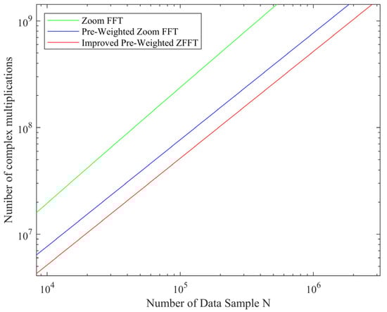
Figure 1.
Comparison of computational complexity of different methods.
3.3. Quadratic Surface Fitting
In Section 3.2, we perform a peak search on the cross-ambiguity function to obtain estimates of time delay and frequency shift. Due to the continuous variation of the time–frequency differences between signals, this method can only provide coarse estimates of TDOA and FDOA [33,34,35]. Therefore, the quadratic surface fitting method is used to improve the accuracy of the time–frequency difference estimation. Assume that the coarse estimated value coordinates of time delay and frequency shift are
The specific steps of quadratic surface fitting are as follows. First, establish a quadratic surface equation as
where are the coefficients to be determined of the fitting function. The eight points around the peak value are recorded to determine these coefficients. By substituting the coordinates of the peak value and the surrounding eight points into the surface equation, the least squares solution for the coefficients can be obtained. By calculating the derivative of Equation (16), we can obtain that the peak coordinates satisfy the relationship, as follows:
After solving the equation, we can obtain the offset of the precise estimation result of the time–frequency difference compared with the original peak value as follows:
Thus, the precise TDOA and FDOA are
3.4. Joint Time–Frequency Difference Localization Method
Based on TDOA, the iso-time-difference hyperbolic surface (a spatial hyperbolic surface with two receiving stations as foci) is determined; based on FDOA, the iso-frequency-difference surface (an ellipsoidal surface with two receiving stations as foci) is determined. Given the earth’s surface equation, calculate its intersection with the iso-time-difference hyperbolic surface and the iso-frequency-difference surface. After removing one of the mirror ambiguity points, the remaining point is the location of the source.
3.4.1. Time–Frequency Difference Localization Model
In the geodetic coordinate system, assume that the primary star coordinate vector is , and its radial velocity is , and assume that the secondary star coordinate vector is , and its radial velocity is . The coordinate vector of the target source is ; thus, the distance between the two receiving stations and the source is
Two receiving stations receive electromagnetic waves from a ground target source. Let the TDOA of the electromagnetic waves at the two receiving stations be , and the FDOA of the received signals be . The electromagnetic wave propagation speed is known to be . The distance difference between the two signals, represented by the TDOA, can be expressed as
Formula (25) is the TDOA measurement equation. By differentiating it, we can obtain
where represents the time difference change rate. If the frequency of the target source signal is , can be measured by the frequency difference , and the relationship between them satisfies the following equation:
By substituting Equation (21) into Equation (20), the FDOA measurement equation can be obtained as
where is the wavelength of the target source signal. Given the Earth’s radius , the coordinates of the target source located on the Earth’s surface satisfy the following equation:
By combining these three equations, a nonlinear set of equations is formed, as follows:
Solving this system of equations allows for the precise localization of the target radiation source. By substituting the coordinates of the two receiving stations and the radiation source into this system, we obtain
3.4.2. Newton’s Method
In this section, we will utilize Newton’s method to solve the roots of nonlinear equations, i.e., the exact coordinates of the target source. The theoretical basis of Newton’s method is to use the Taylor series expansion to approximate the roots of a function and iteratively approach the solution through linear approximation. During the iteration process, the coordinates are updated in the direction of the function’s gradient to find a more precise root [36]. This method is usually very effective when the derivative of the function is easy to calculate, converging rapidly to a solution near the root. The advantage of Newton’s method over analytical methods lies in its more precise positioning results [37].
The accuracy of the positioning of Newton’s method depends on the precision of the initial estimate. With a relatively accurate initial value, it can successfully converge through many iterations. Compared to analytical methods, Newton’s method can achieve superior results. The positioning accuracy of Newton’s iteration is within 10 KM, which is relatively similar to the constrained weighted least squares (CWLS) algorithm, and when the signal-to-noise ratio is above 15 dB, the positioning accuracy of Newton’s iteration can reach 1 KM.
For the nonlinear equation , suppose is the approximate solution, and the function is differentiable near . Then, at can be approximated as a linear equation, as follows:
This equation has a unique solution, denoted as , and Newton’s iteration formula is
According to Section 3.4.1, the TDOA/FDOA positioning equations can be expressed as
Let ,. Then, the coefficient matrix of the differentiated nonlinear equation system F(X) can be expressed as
Substitute into equation . When is satisfied ( is the positioning accuracy), stop iterating. The last iteration result is the positioning result. To prevent the iteration from not stopping due to insufficient accuracy, set the maximum number of iterations as . The coordinate point at the stop of iteration is taken as the solution to the time–frequency difference equation group, i.e., the estimated coordinates of the target source.
4. Hardware Platform Design and Algorithm Implementation
This section introduces the specific engineering implementation process of the joint time–frequency difference positioning algorithm. Section 4.1 will build a signal processing platform and describe its specific structure. Section 4.2 elaborates on the implementation method of the joint time–frequency difference positioning algorithm, including how various modules of the algorithm map to the hardware. In Section 4.3, we present methods to improve the algorithm’s execution efficiency on the DSP platform, which enhance the real-time performance of the time–frequency difference joint positioning system.
4.1. Signal Processing Platform Design
In this section, we build a signal processing platform suitable for the joint time–frequency difference positioning algorithm and complete its hardware implementation. The signal processing platform is constructed following the 6U-CPCI architecture standard. The board is equipped with a CPCI bus interface to establish connections with other functional sub-cards. Simultaneously, the on-board extensive resource FPGA, 8-core DSP, and high-performance SOC enable the transmission of processed results to the host computer via the Ethernet. The processed results are subsequently conveyed through three optical fiber connectors and network ports. The board offers three optical ports, one Gigabit Ethernet port, and two hundred Gigabit Ethernet ports. Given the complexity and parallel nature of the time–frequency difference positioning algorithm, the signal processing platform utilizes Xilinx-Virtex7 series high-performance FPGA and a multi-core DSP developed by the National University of Defense Technology, forming a heterogeneous processing architecture. FPGA is programmed in hardware language, suitable for high line rate transmission, block diagram programming, processing fixed, or repetitive tasks. DSP uses the C language, assembly language programming, floating-point operation ability, and a short development cycle, suitable for dealing with complex multi-thread algorithm tasks. TI provides a wealth of library functions, and provides corresponding function support for each peripheral interface, which is convenient for users to develop. The two high-performance DSPs can perform large-scale, high-precision digital signal processing and are equipped with gigabit Ethernet ports for data exchange with the host computer. The FPGA integrates powerful, flexibly configurable programmable resources for implementing input/output interfaces, general digital logic, memory, and digital signal processing, which are responsible for unpacking instructions and data preprocessing. Each DSP signal processing node is equipped with four DDR3 SDRAM chips, forming a 64-bit width and 2 GB of storage space. The FPGA signal processing node is equipped with two DDR3 SDRAM chips, forming a group with 1GB capacity and 32-bit width storage space, which are used for storing a large amount of intermediate data in the algorithm. Four high-speed 4×SRIO interfaces are mounted between every two processing nodes, enabling high-speed data transmission between the FPGA and DSP, and between the two DSPs. The signal processing platform interacts with the host computer through an Ethernet interface for data exchange, establishing a TCP connection, through which the host computer sends and uploads instructions and data, as well as displays graphics. The picture of the digital signal processing platform is shown in Figure 2.
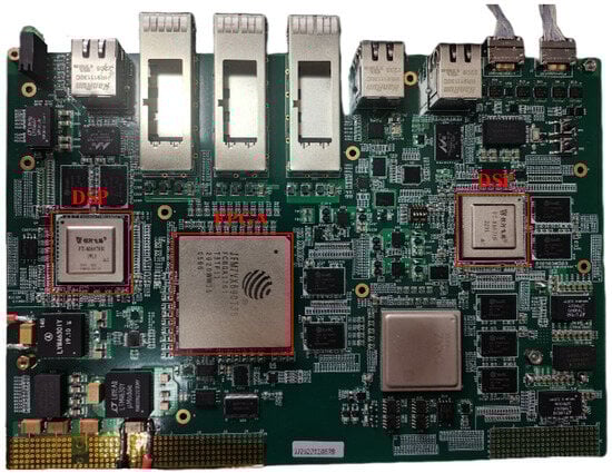
Figure 2.
Picture of the signal processing platform.
4.2. Algorithm Implementation
Based on the algorithm design discussed in Section 3, assume that the minimum and maximum time differences between two receiving data channels are and , respectively. If to is divided into groups, then for any delay , the CAF can be considered as the result of processing the two received data streams and , as shown in Figure 3. After obtaining the CAF, a quadratic surface fitting is performed to accurately estimate the time–frequency difference. Combining this with the parameters of the positioning scenario, the position information of the target source is obtained.
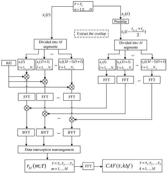
Figure 3.
Calculation flow of CAF for τ with arbitrary delay.
For the joint time–frequency difference positioning algorithm, the algorithm implementation tasks are divided according to the processing advantages of FPGA and DSP. FPGA is suitable for high data rate, parallel operations, and fixed processing tasks in development scenarios, and is therefore used to implement parallel data collection, preprocessing, and mixing product computation in the time–frequency difference positioning algorithm. DSP is suitable for lower data bandwidth, multi-condition operations, complex algorithm tasks, and high-precision digital signal processing scenarios. As a result, it is used to complete the computation of the cross-ambiguity function, peak search, quadratic surface fitting, and the subsequent positioning solution process. Additionally, a dual-DSP architecture is adopted to further divide the computation process to meet the algorithm’s requirements for DSP processing capabilities. The data interaction between each processing node is carried out using a high-speed bus SRIO to achieve a high-speed transmission of data and instructions.
Figure 4 shows the specific implementation flow of the joint time–frequency difference positioning method in FPGA and DSP. FPGA receives two parallel data streams for processing and transmits the mixed product results to DSP1 via SRIO. After signal processing using the DSP1 node, the time–frequency difference estimation results are transmitted to DSP2 to carry out a positioning solution, thus obtaining the target source’s location. The processing results are then transmitted back to the host computer via the Ethernet and are displayed.
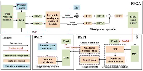
Figure 4.
Algorithm implementation block diagram.
In dual-path data parallel acquisition, data need to be delayed according to the time difference search range. Pre-delay is applied to in parallel data for segments based on prior information, while the starting position of remains unchanged. The relative offset of to for each segment is given by
The pre-delayed and are stored in DDR, and the pre-delay instructions and the subsequent compensatory instructions for segmentation are stored in BRAM.
Since is the delayed input, the excess part at the end of is truncated. Take the overlapping parts of and for subsequent data preprocessing, and write zeros before each piece of data to align it with to facilitate the subsequent division of segments. Assuming a clock period of , we calculate the number of zeros written in the segment of as follows:
Data are read subsequently by controlling the FIFO read and write commands. Two receiving FIFOs acquire and separately. The write clock and read clock of the two receiving FIFOs operate in different clock domains. In the process of selecting the FIFO read and write clocks, the write clock frequency is much lower than the read clock frequency, ensuring that the FIFO does not overflow in the case of discontinuous data reading. The valid signal identifies the effective length of each data segment. The valid signal of the serves as the write enable for both FIFOs. When the rising edge of the valid signal is detected, the write enable for both FIFOs is asserted, allowing the FIFO of the and to perform writing operations. At the same time, this valid signal serves as the flag for the counter to start counting. When the valid signal is high and the valid signal is low, zeros are written into the ’s FIFO. When the rising edge of the valid signal is detected, the counting ends, and the data written into the ’s FIFO switch from zeros to the . This approach achieves truncation and zero padding of the two data paths.
Following the discussion in Section 3 on the fast calculation method for the CAF, we now divide the and into segments, each with a length of , and select points in each data segment. In the read clock domain of the FIFO, by properly designing the width of the read enable, fixed-length data are sequentially read from the receiving FIFO, achieving data segmentation. This process can be expressed as
After calculating with weighted filtering, and are then subjected to FFT processing, complex multiplication processing, and IFFT processing in succession, requiring a total of FFT processing, complex multiplication processing, and inverse FFT processing operations.
As shown in Figure 5, this process employs a pipelining approach to process the segments of data. When the rising edge of the FIFO read command is detected, the data and begin their respective multiplication and FFT calculation processes in sequence. When the FFT calculation results of and are synchronized through the FIFO2 and multiplied, the read command of the FIFO1 is lowered for a period and then raised again. The calculation module detects the rising edge of the FIFO2 read command again, and continues to read the next segment of data. While the first segment of data undergoes subsequent IFFT processing, the second segment of data goes through FFT processing, and the processing of the two segments proceeds simultaneously without affecting each other. This process continues in sequence until all segments of data are processed. This method significantly reduces the algorithm processing time in the FPGA, enhancing data processing efficiency. After processing, a mixing product matrix of size is obtained, as follows:
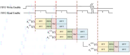
Figure 5.
Pipeline processing flow of segment data.
After completing the mixing product operation, the data are truncated according to the algorithm’s parameters. The processed data are packaged and transmitted to the DDR of the DSP1 through the SRIO. After receiving the doorbell message from the SRIO, the DSP performs matrix transposition and rearrangement of the mixing product data transmitted pulse by pulse via the FPGA and converts the fixed-point data into single-precision floating-point data.
To meet the high real-time requirements of the time–frequency difference positioning algorithm, this paper employs multi-core parallel processing in the DSP. The 0-core of the DSP-M6678 serves as the “main core” responsible for system control and task allocation, while the remaining 7 cores act as computational units participating in calculation tasks. A “Fork-Join” working pattern is employed among the 8 cores. During the FFT processing of the mixing product matrix, a synchronous computation is used among the 8 cores. Data are evenly divided into 8 parts in the frequency-domain dimension, with each core determining its data processing address based on its core number. Since the core’s access speed to L2 SRAM (Level 2 Static Random-Access Memory) is higher than that of DDR SDRAM, the data for each frequency-domain dimension is first moved to L2 SRAM using EDMA. As shown in Figure 6, the FFT calculation and absolute value computation are performed in L2 SRAM, and the results are stored in DDR via EDMA.
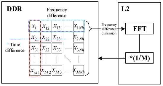
Figure 6.
Frequency difference dimension FFT processing module.
Perform FFT processing on the mixing product matrix to obtain the CAF. The specific implementation formula is
Perform quadratic surface fitting on the discrete CAF, and perform a peak search on the fitting results to obtain a coarse estimate of the time–frequency difference. First, we find the maximum value of each segment of the frequency difference data, resulting in values. Then, we identify the peak value from these values, corresponding to the precise estimates of TDOA and FDOA. Transmit TDOA and FDOA, as well as the coordinates of the receiving stations, to the DSP2 via 4×SRIO. According to the algorithm’s design, the DSP2 calculates the location of the source.
We utilize the Semaphore mechanism provided by TI (Texas Instruments) for C66x CorePacs to implement a multi-core synchronization for shared resources. Semaphores are used to prevent conflicts in the access of shared resources among multiple cores in the data processing flow [38]. Each core in the DSP can acquire semaphores resources in three ways: direct access, indirect access, and combined access. Cores read the SEM_DIRECT register to acquire semaphore values and check the semaphore states of each core. This allows it to determine whether each core’s data processing task is completed.
During a multi-core synchronization operation, all 8 cores simultaneously call the CSL_semAcquireDirect() function to acquire semaphores. In the next synchronization step, all 8 cores simultaneously call the CSL_semReleaseSemaphore() function to release the semaphores. Alternating semaphore acquisition and release achieves multi-core synchronization.
4.3. DSP Program Optimizing
- EDMA transfer optimization: EDMA defines data transfers in three dimensions: ACNT, BCNT, and CCNT. In our program design, EDMA is employed for the continuous movement of mixing product matrices. We use the AB synchronous data transfer mode, with ACNT and BCNT playing crucial roles. As the size of ACNT determines the data block size for a single burst transfer in EDMA, we opt for a larger ACNT parameter to enhance the efficiency of EDMA data transfers.
- Inline function and loop unrolling: The “#pragma UNROLL(n)” directive is used to specify that a particular loop needs to be unrolled n times by the compiler. This allows multiple iterations of the loop body to be copied into the program, folding the loop and improving instruction-level parallelism in the code. In the calculation process of time–frequency difference positioning, operations such as fixed-point to floating-point conversion and spectrum shifting are optimized using inline functions and loop unrolling to reduce the overall execution time.
- Cache optimization: During the calculation of the CAF, data from each segment of frequency difference in the mixing product is sequentially moved into the L2 SRAM for FFT and modulus calculations. The DSP kernel needs to access the L2 SRAM multiple times, and the read and write performance of the L2 SRAM highly depends on L1D. Therefore, we configure the entire L1D as cache to improve the efficiency of data retrieval by the kernel. When the kernel accesses the L2 SRAM multiple times, instruction pipelining can help reduce additional overhead, and the cache coherence of the L2 SRAM is automatically maintained by hardware, eliminating the need for manual maintenance.
5. System Validation
5.1. Time–Frequency Difference Estimation Results
To validate the accuracy of the time–frequency difference localization system’s calculations, we conducted a simulation where two pseudo-random code-modulated BPSK signals were generated. Time delays and Doppler frequency shifts were introduced to BPSK1 and BPSK2. With a sampling rate of 200 kHz, we generated 10,000 data points for joint time–frequency difference estimation and computed the CAF for the two signals. The specific simulation parameters are shown in Table 1:

Table 1.
Simulation parameters for typical scenarios in TDOA/FDOA localization.
MATLAB is used for algorithm simulation analysis. The TDOA estimation is 0.0002 s, and the FDOA estimation is −0.00009722598 Hz. The simulation results of the CAF are shown in Figure 7:
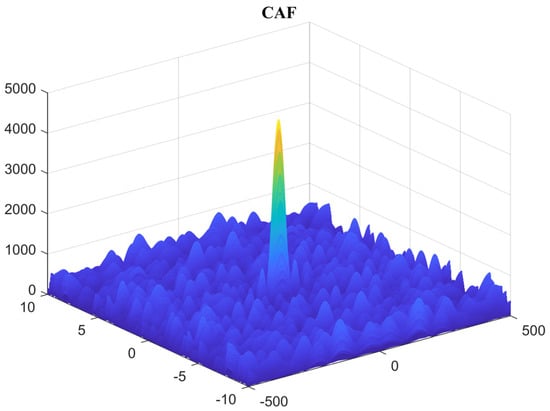
Figure 7.
Cross−ambiguity function result.
In the figure, the x-axis and y-axis, respectively, represent the time difference correction value and the frequency difference correction value. We validate the time–frequency difference localization algorithm on the signal processing platform. The time–frequency difference estimates calculated by the signal processing platform are compared with the simulated results, as shown in Table 2.
Table 2.
Time–frequency difference positioning results.
The difference between hardware results and simulation results mainly comes from the following reasons:
- Data format: MATLAB’s data format comprises double-precision floating-point numbers, while hardware (DSP and FPGA) uses fixed-point numbers and single-precision floating-point numbers.
- Programming language characteristics: The underlying logic of the programming language used by DSP and FPGA is different from that used by a MATLAB simulation, which also affects their different rounding and truncation strategies when processing numerical values, resulting in cumulative errors.
The comparative results indicate that the accuracy of FDOA is between 10−7 and 10−8, and the accuracy of TDOA can be maintained between 0.1 us and 0.01 us. The positioning results are in good agreement with the simulated calculations, which satisfies the precision requirements for practical applications, thus validating the correctness and effectiveness of the joint time–frequency difference localization processing platform presented in this paper.
5.2. Real-Time Performance Analysis
Since core 0 arranges the tasks of other cores, statistical time performance is based on core 0. The time measurement tools used comprise the timestamp registers (TSCL, TSCH) from the TI library, and the DSP operates with a clock frequency of 1.0 GHz. Table 3 provides the execution time statistics for each module before and after DSP program optimization.
Table 3.
Execution time of each calculation module.
6. Conclusions
This paper investigates issues related to passive localization methods and hardware platform implementation. First, we elaborate on the signal processing flow of time–frequency difference localization and enhance the PW-ZFFT method by using a frequency-domain approach to calculate the mixing product, thereby reducing the computation load of the CAF. Then, we construct a heterogeneous signal processing platform based on FPGA and DSP, and determine the engineering task division and implementation of the algorithm flow based on the signal processing capabilities and advantages of FPGA and multi-core DSP. Considering the characteristics of data, we design methods to enhance program performance based on the DSP platform. Through the simulation of typical scenarios and hardware measurement results, the performance analysis of the time–frequency difference’s passive localization processing unit is conducted, which validates the correctness and real-time capability of the program.
Author Contributions
Conceptualization, G.X. and Q.D.; methodology, G.X. and Q.D.; software, G.X. and Q.D.; validation, G.X. and Q.D.; formal analysis, G.X.; investigation, G.L.; resources, G.X.; data curation, Q.D.; writing—original draft preparation, G.X. and Q.D.; writing—review and editing, K.X. and G.L.; visualization, S.L.; supervision, G.L.; project administration, G.X.; funding acquisition, Y.Q. All authors have read and agreed to the published version of the manuscript.
Funding
This work is supported in part by the National Natural Science Foundation of China (62331019) and in part by the Science Funds for Distinguished Young Scholars of Shaanxi Province (2021JC-23).
Data Availability Statement
Data are contained within the article.
Acknowledgments
The authors are grateful to the XiDian University for supporting this research. The authors are also grateful to the associate editor who provided valuable insights and intriguing discussions during this study. Your diverse perspectives and collaborative spirit greatly enriched the research experience.
Conflicts of Interest
The authors declare no conflicts of interests.
References
- Devi, M.; Dhabale, N.R. Active and Passive Radar-Location Systems for the Calculation of Coordinates. In Proceedings of the 2017 International Conference on Innovative Mechanisms for Industry Applications (ICIMIA) 2017, Bengaluru, India, 21–23 February 2017; pp. 770–773. [Google Scholar]
- Antonyuk, V.; Prudyus, I.; Nichoga, V.; Kawalec, A. Integration of Passive Coherent Radar System into the Passive TDOA System. In Proceedings of the 2012 13th International Radar Symposium, Warsaw, Poland, 23–25 May 2012; pp. 354–358. [Google Scholar]
- Zhu, Y.; Zhang, S. Passive Location Based on an Accurate Doppler Measurement by Single Satellite. In Proceedings of the 2017 IEEE Radar Conference (RadarConf), Seattle, WA, USA, 8–12 May 2017; pp. 1424–1427. [Google Scholar]
- Wu, H.; Wu, Z.-H.; Shi, Z.-S.; Sun, S.-Y. Research on Multi-Moving Target Location Algorithm Based on Improved TDOA/FDOA. Meas. Control 2023, 56, 938–952. [Google Scholar] [CrossRef]
- Sun, P.; Zhang, G.; Qu, D.; Ji, H.; Guo, H. Cross Ambiguity Function Interpolation Algorithm for FDOA Estimation of Signal Location. In Proceedings of the 2019 IEEE 11th International Conference on Communication Software and Networks (ICCSN), Chongqing, China, 12–15 June 2019; pp. 202–205. [Google Scholar]
- A Joint TDOA, FDOA and Doppler Rate Parameters Estimation Method and Its Performance Analysis|IEEE Conference Publication|IEEE Xplore. Available online: https://ieeexplore.ieee.org/document/8855429 (accessed on 19 December 2023).
- Huang, L.; Zhang, Y.; Li, Q.; Pan, C.; Song, J. Fast Calculation for Cross Ambiguity Function in Passive Detection Systems. In Proceedings of the 2018 International Conference on Sensing, Diagnostics, Prognostics, and Control (SDPC), Xi’an, China, 15–17 August 2018; pp. 690–694. [Google Scholar]
- Junjie, L.; You, H.; Jie, S. The Algorithms and Performance Analysis of Cross Ambiguity Function. In Proceedings of the 2009 IET International Radar Conference, Guilin, China, 20–22 April 2009; pp. 1–4. [Google Scholar]
- Kim, D.-G.; Park, G.-H.; Kim, H.-N.; Park, J.-O.; Park, Y.-M.; Shin, W.-H. Computationally Efficient TDOA/FDOA Estimation for Unknown Communication Signals in Electronic Warfare Systems. IEEE Trans. Aerosp. Electron. Syst. 2018, 54, 77–89. [Google Scholar] [CrossRef]
- Shin, D.C.; Nikias, C.L. Complex Ambiguity Functions Using Nonstationary Higher Order Cumulant Estimates. IEEE Trans. Signal Process. 1995, 43, 2649–2664. [Google Scholar] [CrossRef]
- Ulman, R.; Geraniotis, E. Wideband TDOA/FDOA Processing Using Summation of Short-Time CAF’s. IEEE Trans. Signal Process. 1999, 47, 3193–3200. [Google Scholar] [CrossRef] [PubMed]
- Ho, K.C.; Xu, W. An Accurate Algebraic Solution for Moving Source Location Using TDOA and FDOA Measurements. IEEE Trans. Signal Process. 2004, 52, 2453–2463. [Google Scholar] [CrossRef]
- Yu, H.; Huang, G.; Gao, J.; Liu, B. An Efficient Constrained Weighted Least Squares Algorithm for Moving Source Location Using TDOA and FDOA Measurements. IEEE Trans. Wirel. Commun. 2012, 11, 44–47. [Google Scholar] [CrossRef]
- Sun, X.; Li, J.; Huang, P.; Pang, J. Total Least-Squares Solution of Active Target Localization Using TDOA and FDOA Measurements in WSN. In Proceedings of the 22nd International Conference on Advanced Information Networking and Applications—Workshops (aina workshops 2008), Gino-wan, Japan, 25–28 March 2008; pp. 995–999. [Google Scholar]
- Zheng, L.; Wang, X. Super-Resolution Delay-Doppler Estimation for OFDM Passive Radar. IEEE Trans. Signal Process. 2017, 65, 2197–2210. [Google Scholar] [CrossRef]
- Fuyang, G.U.O.; Zijing, Z.; Linsen, Y. TDOA/FDOA estimation algorithm for linear frequency modulated signals. Chin. J. Radio Sci. 2016, 31, 166–172. [Google Scholar]
- Hu, D.; Huang, Z.; Liang, K.; Zhang, S. Coherent TDOA/FDOA Estimation Method for Frequency-Hopping Signal. In Proceedings of the 2016 8th International Conference on Wireless Communications & Signal Processing (WCSP), Yangzhou, China, 13–15 October 2016; pp. 1–5. [Google Scholar]
- Kumarasiri, R.; Alshamaileh, K.; Tran, N.H.; Devabhaktuni, V. An Improved Hybrid RSS/TDOA Wireless Sensors Localization Technique Utilizing Wi-Fi Networks. Mobile Netw. Appl. 2016, 21, 286–295. [Google Scholar] [CrossRef]
- Zhang, R.; Xia, W.; Yan, F.; Shen, L. A Single-Site Positioning Method Based on TOA and DOA Estimation Using Virtual Stations in NLOS Environment. China Commun. 2019, 16, 146–159. [Google Scholar]
- Wang, Y.; Ho, K.C. Unified Near-Field and Far-Field Localization for AOA and Hybrid AOA-TDOA Positionings. IEEE Trans. Wireless Commun. 2018, 17, 1242–1254. [Google Scholar] [CrossRef]
- Feng, C.; Au, W.S.A.; Valaee, S.; Tan, Z. Received-Signal-Strength-Based Indoor Positioning Using Compressive Sensing. IEEE Trans. on Mobile Comput. 2012, 11, 1983–1993. [Google Scholar] [CrossRef]
- Zhao, C.; Zhao, Y. One Recurrent Neural Networks Solution for Passive Localization. Neural Process Lett. 2019, 49, 787–796. [Google Scholar] [CrossRef]
- Huang, G.; Xi, Z.; Zhou, Y.; Zhou, J. A Novel TDOA Location Algorithm for Passive Radar. In Proceedings of the 2006 CIE International Conference on Radar, 2006, Shanghai, China, 16–19 October 2006; pp. 1–4. [Google Scholar]
- Qu, F.; Guo, F.; Jiang, W.; Meng, X. Constrained Location Algorithms Based on Total Least Squares Method Using TDOA and FDOA Measurements. In Proceedings of the International Conference on Automatic Control and Artificial Intelligence (ACAI 2012), Xiamen, China, 3–5 March 2012; pp. 689–692. [Google Scholar]
- Shilong, W.; Jingqing, L.; Liangliang, G. Joint FDOA and TDOA Location Algorithm and Performance Analysis of Dual-Satellite Formations. In Proceedings of the 2010 2nd International Conference on Signal Processing Systems, Dalian, China, 5–6 July 2010; Volume 2, pp. V2-339–V2-342. [Google Scholar]
- Wang, K.; Chen, Z.; Yan, Q. Research on Multi-Platform Time Difference of Arrival and Frequency Difference of Arrival Joint Location Technology. In Proceedings of the 2021 IEEE 6th International Conference on Signal and Image Processing (ICSIP), Nanjing, China, 22–24 October 2021; pp. 563–567. [Google Scholar]
- Overfield, J.; Biskaduros, Z.; Buehrer, R.M. Geolocation of MIMO Signals Using the Cross Ambiguity Function and TDOA/FDOA. In Proceedings of the 2012 IEEE International Conference on Communications (ICC), Ottawa, ON, Canada, 10–15 June 2012. [Google Scholar]
- One Intelligent Algorithm for Estimation of TDOA and FDOA|IEEE Conference Publication|IEEE Xplore. Available online: https://ieeexplore.ieee.org/document/7065099 (accessed on 22 December 2023).
- Research on Fast Computation of Ambiguity Function|IEEE Conference Publication|IEEE Xplore. Available online: https://ieeexplore.ieee.org/document/4566145 (accessed on 22 December 2023).
- A Fast Method for Time Delay, Doppler Shift and Doppler Rate Estimation|IEEE Conference Publication|IEEE Xplore. Available online: https://ieeexplore.ieee.org/document/4148486 (accessed on 22 December 2023).
- Wei-qiang, Z.; Rau, T.; Yong-feng, M. Fast Computation of the Ambiguity Function. In Proceedings 7th International Conference on Signal Processing, 2004. Proceedings. ICSP ’04. 2004, Beijing, China, 31 August–4 September 2004; IEEE: Beijing, China, 2004; Volume 3, pp. 2124–2127. [Google Scholar]
- Deng, L.; Leng, K. Application of Two Spectrum Refinement Methods in Frequency Estimation. J. Phys. Conf. Ser. 2022, 2290, 012070. [Google Scholar] [CrossRef]
- Stein, S. Algorithms for Ambiguity Function Processing. IEEE Trans. Acoust. Speech Signal Process. 1981, 29, 588–599. [Google Scholar] [CrossRef]
- Tao, R.; Zhang, W.-Q.; Chen, E.-Q. Two-Stage Method for Joint Time Delay and Doppler Shift Estimation. IET Radar Sonar Amp Navig. 2008, 2, 71–77. [Google Scholar] [CrossRef]
- Jiang, F.; Zhang, Z.; Esmaeili Najafabadi, H.; Yang, Y. Underwater TDOA/FDOA Joint Localisation Method Based on Cross-Ambiguity Function. IET Radar Sonar Navig. 2020, 14, 1256–1266. [Google Scholar] [CrossRef]
- Target Location Based on Quasi-Newton Algorithm in Multistatic Passive Radar|IET Conference Publication|IEEE Xplore. Available online: https://ieeexplore.ieee.org/document/7455659 (accessed on 22 December 2023).
- Joint Estimation of Time Delay and Doppler Shift for Band-Limited Signals|IEEE Journals & Magazine|IEEE Xplore. Available online: https://ieeexplore.ieee.org/document/5471174 (accessed on 22 December 2023).
- TMS320C6678 Optimizing Compiler v7.4 User’s Guide; Texas Instruments Incorporated: Dallas, TX, USA, 2012.


Disclaimer/Publisher’s Note: The statements, opinions and data contained in all publications are solely those of the individual author(s) and contributor(s) and not of MDPI and/or the editor(s). MDPI and/or the editor(s) disclaim responsibility for any injury to people or property resulting from any ideas, methods, instructions or products referred to in the content. |
© 2024 by the authors. Licensee MDPI, Basel, Switzerland. This article is an open access article distributed under the terms and conditions of the Creative Commons Attribution (CC BY) license (https://creativecommons.org/licenses/by/4.0/).