Abstract
The Ganges–Brahmaputra estuary, located in the northern Bay of Bengal, is situated within the largest delta in the world. This river basin features a complex river system, a dense population, and significant variation in watershed vegetation cover. Human activities have significantly impacted the concentration of total suspended matter (TSM) in the estuary and the ecological environment of the adjacent bay. In this study, we utilised the Landsat series of satellite remote sensing data from 1990 to 2020 for TSM retrieval. We applied an atmospheric correction algorithm based on the general purpose exact Rayleigh scattering look-up-table (LUT) and the shortwave-infrared (SWIR) bands extrapolation to Landsat L1 products to obtain high-precision remote sensing reflectance. In conjunction with the normalised difference vegetation index (NDVI), precipitation, and discharge data, we analysed the variation and influencing mechanisms of TSM in the Ganges–Brahmaputra estuary and its surrounding areas. We revealed notable seasonal variation in TSM in the estuary, with higher concentrations during the wet season (May–October) compared to the dry season (the rest of the year). Over the period from 1990 to 2020, the NDVI in the watershed exhibited a significant upward trend. The outer estuarine regions of the Hooghly River and Meghna River displayed significant decreases in TSM, whereas the Baleswar River, which flows through mangrove areas, showed no significant trend in TSM. The declining trend in TSM was mainly attributed to land-use changes and anthropogenic activities, including the construction of embankments, dams, and mangrove conservation efforts, rather than to runoff and precipitation. Surface sediment concentration and chlorophyll in the northern Bay of Bengal exhibited slight increases, which means the limited influence of terrestrial inputs on long-term change in surface sediment concentration and chlorophyll in the northern Bay of Bengal. This study emphasises the impact of human activities on the river–estuary–coast continuum and sheds light on future sustainable management.
1. Introduction
The Ganges–Brahmaputra River system, located in the northern Bay of Bengal, is one of the most significant river systems in the world. It encompasses a total drainage area of approximately 1.7 million square kilometres [1,2,3]. The annual average discharge of the Ganges and Brahmaputra rivers into the northern Bay of Bengal is around 1350 km3 [4,5]. These rivers transport approximately 1 × 10⁹ t yr−1 of sediment to the Ganges–Brahmaputra delta [6], making it one of the largest river sediment delivery systems in the world. The delta is characterised by an intricate network of rivers, including the major systems like the Hooghly River, Meghna River, and tributary channels represented by the Baleswar River [7,8,9]. The sediments carried by these rivers continuously deposit in the estuary, resulting in the formation of a fertile and densely populated delta and wetland system [10]. The population of the basin is approximately 150 million [11], making it one of the most densely populated deltas in the world [12]. Due to the influence of global warming, the rising sea level threatens the coasts of the Ganges–Brahmaputra delta [13]. Therefore, the substantial amount of sediment transported by the river system plays a critical role in mitigating land erosion. Additionally, in the downstream part of the Ganges–Brahmaputra delta, the world’s largest mangrove system, the Sundarbans [14], covers an area of approximately 10,000 km2 [15]. The supplies of fresh water and sediment in the mangroves significantly impact the health of the regional mangrove ecosystem [16]. The interaction between river discharge and tides results in the unique and complex ecological environment of the coastal waters in the northern Bay of Bengal [17].
The concentration of total suspended matter (TSM) reflects the content of suspended particles in water and is one of the key parameters for studying suspended sediment transport and for studying water quality and ecological environment in rivers and coastal waters [18]. TSM is an important parameter of the transports of carbon, nutrients, pollutants, and other substances [19,20,21]. In estuarine regions, TSM concentration is typically high due to land inputs and sediment resuspension. As a result, the potential impacts of suspended sediments on marine ecosystems in such regions have gained increasing scientific attention [10,22,23,24,25]. Under the combined pressure of human activities and climate change, TSM serves as an indicator of erosion, land-use changes, and sediment transport. More importantly, TSM is crucial for understanding the stability of delta coastlines and its impact on the coastal ecological environment.
Some early studies based on in situ measurements provided valuable insights into the suspended sediment load and flux of different rivers in the Ganges basin [26,27,28]. Abbas and Subramanian (1984) [26] calculated the annual suspended sediment input to the Hooghly estuary, which could reach 328 × 106 t yr−1. The authors suggested that variation in sediment concentration in the water were primarily due to dilution by low sediment from tributaries upstream and the regulation of river flow and sediment by dams. Jha et al. (1988) [27] conducted seasonal measurements of sediment concentration in the Yamuna River (upstream of the Hooghly River) and found that the highest sediment transport occurred during the monsoon season (June–September), which corresponds to the wet season in the Ganges–Brahmaputra delta [29]. Sediment load constituted 58–86% of the total load carried by the Ganges–Brahmaputra River, depending on the location. Barua (1990) [28] measured the suspended sediment concentration in turbidity maximum at the mouth of the Ganges–Brahmaputra–Meghna river system in Bangladesh. The author found that suspended sediments were net input via flood channels and net output through ebb channels in the river channels. These early studies provided important data on sediment dynamics in the Ganges basin, shedding light on the seasonal and tidal variation in sediment transport.
Although some achievements have been obtained based on in situ measurements, these measurements are limited by the scarcity of sampling sites and can hardly reflect the situation of the entire region. Moreover, estimating TSM in coastal waters using traditional field sampling methods is time-consuming and costly, and it is difficult to acquire long-term, large-scale data. In contrast, satellite remote sensing offers a more convenient alternative [30,31] due to its easy acquisition and wide coverage [32]. A close relationship between suspended sediments and spectral band ratios (e.g., between near-infrared and blue, between red and green, between near-infrared and red) is reported [33,34,35,36], as well as of the TSM with the red band [37]. These relationships can be used for the retrieval of suspended sediment concentration [38]. Examples of relevant satellite bands include Landsat band 3, Landsat 8 band 4, and MODIS band 1 [37,39,40,41,42,43].
Islam et al. (2001) [37] established a linear algorithm for suspended sediment concentration based on the Landsat Thematic Mapper (TM) red band reflectance in the Ganges–Brahmaputra River basin and the Ganges–Brahmaputra estuary region. This algorithm was developed using in situ measurements conducted by the Bangladesh Water Development Board (BWDB) at locations in the Ganges and Brahmaputra Rivers, specifically at Hardinge Bridge and Bahadurabad Ghat. The authors analysed the suspended sediment concentration of the Ganges and Brahmaputra rivers during high and low flow periods. They found that during high-flow periods, the Ganges had a higher suspended sediment concentration, and, during low-flow periods, the Brahmaputra exhibited a higher concentration. Islam et al. (2002) [44] extended the research to estimate the suspended sediment concentration in the Bay of Bengal. They discovered that during low-flow periods, the outermost region of turbidity maximum was closer to the coast. However, during high-flow periods, the turbidity maximum extended into coastal waters, resulting in significant seasonal variation in suspended sediment concentration in the coastal area (between 5 m and 10 m isobaths). Yan and Tang (2009) [10] used MODIS data to investigate the spatiotemporal change in suspended sediment concentration in the Bay of Bengal following the Sumatra tsunami in 2004. Their findings revealed a short-term increase in the suspended sediment concentration at major river mouths along the coast, particularly along the northwest coast of Indonesia, the southeast coast of Myanmar, and the northern coast of the Bay of Bengal. Based on MODIS and Landsat satellite data, and in situ TSM measurements from multiple monitoring stations during 2016–2019, Sahoo et al. (2022) [45] developed a single-band algorithm for estimating TSM in the urban section of the Hooghly River, a tributary of the Ganges. This algorithm enables the wide-scale acquisition of water quality parameters in urban river sections. While these studies provided insights into sediment distribution patterns during dry and wet seasons and the influence of episodic weather events on TSM, the long-term change in suspended sediment transport in the region has not yet been investigated due to the lack of continuous, long-term data. Furthermore, many of these studies predominantly focused on meteorological and hydrological conditions, such as precipitation and river flow, with few taking human activities into account.
The northern Bay of Bengal receives a substantial inflow of freshwater and sediment from the Ganges–Brahmaputra River system. This region is characterised by extensive water–sediment transport, and is strongly influenced by monsoons, making it a unique and interconnected system involving oceanography, biology, and sedimentary processes [18]. The area holds significant economic importance for coastal and marine fisheries [46]. However, due to its low elevation, it is also susceptible to impacts of natural disasters [47]. So far, research on the co-evolution of the marine ecosystem in the northern Bay of Bengal and the sediment transport from the Ganges–Brahmaputra River system is limited, particularly regarding the impact of river-borne suspended sediment transport on the ecological environment in the bay.
In the study, we investigated seasonal and interannual variation in TSM in the Ganges–Brahmaputra basin, estuary, and nearshore regions. First, we utilised 30 m spatial resolution Landsat data and a novel high spatiotemporal resolution atmospheric correction algorithm to obtain accurate remote sensing radiance information of water bodies. This information was then used for the retrieval of estuarine TSM from 1990 to 2020. We also analysed the time series data of the basin normalised difference vegetation index (NDVI), basin precipitation, and discharge. In the northern Bay of Bengal, we examined the temporal variation in chlorophyll concentration and surface sediment concentration using MODIS satellite products from 2010 to 2020. Finally, we discussed the changes and interrelated mechanisms within the entire river–estuary–coast continuum.
2. Materials and Methods
2.1. Study Area
The study area encompasses the Ganges–Brahmaputra delta, Ganges–Brahmaputra estuary, and the northern Bay of Bengal, namely within the region of 87.5–91.5°E, 20–23.5°N (as depicted in Figure 1). The Ganges–Brahmaputra River basin comprises three major river systems, namely the Ganges River, Brahmaputra River, and Meghna River, which are strongly influenced by monsoons [48]. These three river systems converge within the Ganges–Brahmaputra delta before entering the northern Bay of Bengal, collectively forming one of the world’s largest river discharge systems, with an annual discharge of approximately 1350 km3 [5,49].
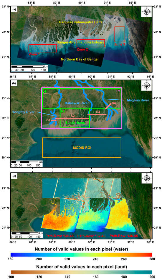
Figure 1.
Study area, regions of interest (ROIs), and the number of valid values of satellite data. (a) The study area includes the downstream Ganges–Brahmaputra delta, Ganges–Brahmaputra estuary, and the northern Bay of Bengal. The red boxes, Zone 1 (87.9–89°E, 21.2–21.5°N), Zone 2 (89.8–90.9°E, 21.4–21.7°N), and Zone 3 (91.3–91.7°E, 21.6–22.2°N), indicate the ROIs for the TSM time series statistics. (b) The purple box (“Pr”, 87.5–91.5°E, 21.5–23.5°N) represents the area for precipitation statistics. The blue lines denote the three major river channels of the Ganges–Brahmaputra delta: Baleswar River, Hooghly River, and Meghna River, with the four sections in the estuaries for discharge data statistics (red lines), labelled as S1 (87.975–88.175°E, 21.875°N), S2 (88.175–89.825°E, 21.975°N), S3 (89.825–90.725°E, 22.175°N), and S4 (90.725°E, 22.475°N to 90.975°E, 22.725°N), respectively. The green box represents the region for NDVI calculation, where N1 corresponds to the upstream delta region (87.5–91.5°E, 22.5–23.5°N) and N2 corresponds to the Sundarbans mangrove reserve (88.4–89.9°E, 21.5–22.5°N). The orange box (MODIS-ROI) is the ROI statistical area of the northern Bay of Bengal (87.5–91.5°E, 20–21°N). (c) The number of valid values in each pixel. The number of valid values on land and in the ocean are separately counted. The land area statistics cover the valid value count within the “N1” and “N2” mentioned in (a), while the ocean area statistics include the valid value count for the three Landsat scenes shown in (b). The WRS path/row of each Landsat satellite scenes used for TSM inversion is marked in red.
The predominant climate type in this region is tropical monsoon climate, characterised by distinct wet and dry seasons. The wet season spans from May to October, while the dry season encompasses November to April of the following year [29]. The annual average precipitation in this area is approximately 1809.4 mm [47]. The monsoon season, occurring from June to September is marked by the heaviest and most concentrated precipitation, contributing to 60–90% of the annual precipitation [48]; it exceeds 1200 mm month−1. In contrast, the winter season experiences much lower precipitation, typically less than 50 mm month−1. The monsoonal rainfall pattern profoundly influences the river discharge in the Ganges–Brahmaputra delta. Generally, the peak flow is in July and August, with occasional flood events occurring in September in some river segments [49,50].
2.2. Landsat Data
In this study, we use the Landsat series, including Landsat 8 Operational Land Imager (OLI) and Thermal Infrared Sensor (TIRS) Level 1 (L1) products, as well as the Landsat 5 Thematic Mapper (TM) Level 1 products. The data from 1990 to 2020 (not including 2002 and 2012 due to unavailability) were obtained from the U.S. Geological Survey (USGS) at https://earthexplorer.usgs.gov/ (accessed on 4 September 2022) [51]. We selected the Collection 2 Tier 1 dataset, which were placed with the highest quality Landsat scenes and suitable for time series analysis [52].
The specific Landsat World Reference System (WRS) paths and row chosen for analysis are 136–138 and 45, respectively, as depicted in Figure 1c. To ensure data quality, only images with cloud cover less than 20% were selected for further analysis, resulting in a total of 854 images. The number of valid data in each pixel varied, as illustrated in Figure 1c. The images used for the retrieval of TSM exhibited consistent validity, with more than 220 valid values observed over the 31-year period. Images from path/row 138/45 had the highest count of valid data points, followed by those from path/row 136/45, and those from path/row 137/45 were lowest. Because there are offsets in image positions during each capture, fewer valid data counts were observed at the edges of the images, especially in the southeast corner of each image. Therefore, when selecting the region of interest (ROI) for analysing the temporal variation in TSM, we chose the ROI in areas with a higher count of valid data, marked by the red boxes in Figure 1a.
The numbers of available satellite images during the dry season (January–April and November–December) and the wet season (May–October) were counted (Figure 2). Over the three decades, a gradual increase in the volume of available data can been seen. It is evident that more data were acquired during the dry season compared to the wet season. This difference is likely due to frequent cloudy and rainy days in the wet season. However, even during the wet season when data acquisition was less frequent, it was still feasible to secure a minimum of nine images for analysis.
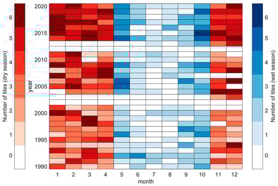
Figure 2.
Number of Landsat scenes in each month during 1990–2020, as indicated in Figure 1a. The red and the blue colour bars represent the valid number of scenes captured during the dry and wet seasons, respectively.
2.3. MODIS Data
We obtained monthly surface sediment concentration and chlorophyll products from the Western Pacific–Indian Ocean dataset provided by the Marine Satellite Data Online Analysis Platform SatCO2 (https://www.satco2.com/ (accessed on 30 August 2023)) [53]). They covered the period from May 2010 to December 2020. This dataset is a fusion of data from EOS/MODIS and China’s HY-1B satellite. The estimate of chlorophyll concentration in the dataset was based on an empirical algorithm using the blue–green band ratio [54,55], while surface sediment concentration was estimated using an empirical model [54,55,56]. A specific ROI labelled as “MODIS-ROI” (see Figure 1b), from 87.5–91.5°E and 20–21°N, was selected to represent the primary productivity and suspended sediment condition within the continental shelf of the northern Bay of Bengal.
2.4. Hydrological Data
We utilised river discharge data from the Global Flood Awareness System (GloFAS) 4.0 dataset, available from the Climate Data Store by the ECMWF [57]. This dataset was generated using ERA5 meteorological reanalysis data and the open-source LISFLOOD hydrological model, with interpolation to a 24 h time step. The dataset is organised on a regular latitude–longitude grid with a spatial resolution of 0.05° × 0.05°. We focused on a specific geographical area defined by the coordinates from 87.3°E to 92.7°E and from 22.7°N to 20.7°N. As shown in Figure 1b, we used the analysis of river discharge data at four distinct cross-sections, spanning three significant river estuaries: the Hooghly River, Baleswar River loop structure, and Meghna River. These four sections are referred to as S1 (87.975–88.175°E, 21.875°N), S2 (88.175–89.825°E, 21.975°N), S3 (89.825–90.725°E, 22.175°N), and S4 (90.725°E, 22.475°N to 90.975°E, 22.725°N), respectively.
Precipitation data were sourced from the Global Precipitation Climatology Project (GPCP) Monthly product, namely GPCP Version 3.2 Satellite-Gauge (SG) Combined Precipitation Data Set [58]. The product combines measurements from microwave, infrared, and ground-based rain gauge observations. The monthly averaged data with a spatial resolution of 0.5° × 0.5° from 1990 to 2020 was downloaded from the Earth Data Search platform (https://search.earthdata.nasa.gov/search (accessed on accessed on 30 August 2023) [59]). As illustrated in Figure 1b, the study focused on the land area within 87.5–91.5°E and 21.5–23.5°N for precipitation analysis, denoted as Pr.
2.5. Atmospheric Correction of Landsat Data
The atmospheric correction algorithm for remote sensing products plays a pivotal role in the accurate computation of high-precision radiometric information over water bodies and is a significant limiting factor in aquatic remote sensing [60]. Coastal waters are often highly turbid due to sediment input and resuspension [61], which challenges the precision of atmospheric correction in remote sensing imagery [62]. High spatial resolution remote sensing images differ from traditional ocean colour satellites in terms of band settings. Due to factors such as wide spectral bandwidth and low signal-to-noise ratios, the official Landsat atmospheric correction algorithm is usually assumed to be noneffective in highly turbid waters, resulting in decreased accuracy for water applications [63].
We employed the atmospheric correction algorithm used by Zhang et al. (2023) [64]. This algorithm utilises a general exact Rayleigh scattering look-up-table (LUT) provided by He et al. (2006, 2010) [65,66] to calculate Rayleigh scattering, while neglecting the water-leaving radiance at the shortwave-infrared bands (SWIR) [67,68]. For the visible light and near-infrared (NIR) bands, it employs an extrapolation method with the SWIR bands (Band 5 and Band 7 for Landsat 5, and Band 6 and Band 7 for Landsat 8) to calculate aerosol reflectance.
Additionally, we utilised TSM data generated using the Landsat Collection 2 Surface Reflectance (SR) dataset, whose atmospheric correction algorithm is based on the 6S model [69,70]. We found that the atmospheric correction algorithm employed in this study exhibited better performance than that of the 6S model. For more detail, readers are referred to Section 2.6 and Section 3.1.
2.6. TSM Inversion Model
We retrieved TSM using a universal multi-sensor algorithm proposed by Nechad et al. (2010) [71]. This algorithm establishes a nonlinear empirical model based on the red band water-leaving reflectance and introduces corresponding empirical coefficients for different wavelengths. The algorithm was developed and calibrated based on two independent datasets [72,73] and is applicable to various sensors and wavelengths [74]. It has been applied in the Ganges River basin [42,75]. C. Jayaram et al. (2021) [75] validated this algorithm using field measurements and reported a root-mean-square error (RMSE) of 10.89 mg L–1, indicating a favourable level of regional applicability and accuracy. Hence, we employed this algorithm to retrieve TSM concentration in this study.
The calculation is as follows:
where is water-leaving reflectance and Rrs is the remote sensing reflectance at wavelength λ. For Landsat-5, is at 560 nm, = 327.84, and = 0.1708; for Landsat-8, is at 655 nm, = 289.29, and = 0.1686.
2.7. Normalised Difference Vegetation Index (NDVI)
The NDVI is a commonly used parameter for characterising vegetation cover [76]. It is calculated using the reflectance values in the near-infrared and red bands of remote sensing imagery, as expressed by the following formula [77]:
where NIR represents the reflectance in the near-infrared band and R represents the reflectance in the red band. For Landsat 5 imagery, NIR corresponds to band 4 and R corresponds to band 3. For Landsat 8 imagery, NIR corresponds to band 5 and R corresponds to band 4.
The range of NDVI is [−1, 1]. Negative NDVI indicates surfaces with high reflectance in the visible spectrum, such as water bodies or clouds. Positive NDVI represents vegetated surfaces, with values increasing with higher vegetation cover. NDVI = 0 corresponds to non-vegetated, bare soil surface. NDVI is closely associated with numerous vegetation parameters and serves as a critical indicator for monitoring changes in ground-level vegetation [78].
Unlike water parameter retrievals, the NDVI is less affected by atmospheric correction. To facilitate statistical calculations, we utilised the Landsat Collection 2 L2 Surface Reflectance (SR) dataset within the Google Earth Engine (GEE) platform. We selected images with cloud cover less than 20% and focused on two specific regions (indicated in Figure 1b: the upstream area of the Ganges–Brahmaputra delta (box N1: 87.5–91.5°E, 22.5–23.5°N) and the Sundarbans mangrove reserve area (box N2: 88.4–89.9°E, 21.5–22.5°N). Monthly average NDVI was calculated for these regions.
The spatial distribution of the number of valid NDVI pixels is shown in Figure 1c. The images used for the NDVI calculation generally had more than 160 valid values, and the distribution of valid pixel counts was relatively uniform, with a slight increase in the west and a slight decrease in the east. Since the calculation of NDVI required the mosaicking of multiple images for each region, we took the monthly average NDVI value for each region as a representative value to reduce NDVI biases caused by different image coverages.
3. Results
3.1. Temporal-Spatial Variation in TSM in the Ganges–Brahmaputra Estuary
Seasonal climatology of TSM concentration was obtained by averaging all available data of corresponding seasons (Figure 3). Seasons are defined as winter (December, January, February), spring (March to May), summer (June to August), and autumn (September to November) in this study. The TSM in the Ganges–Brahmaputra estuary exhibits a decreasing trend from the river mouth towards the open ocean, and a high–low–high pattern from the east to west. The turbidity maximum at the Hooghly River appears at its river mouth, while the turbidity maximum in other areas extends to the sea, with TSM concentration exceeding 120 mg L−1. The observation indicates varying levels of resuspended terrestrial sediments originating from upstream regions as carried by river inflow.
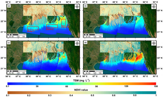
Figure 3.
Seasonal spatial distribution of TSM and NDVI in (a) winter (December to February); (b) spring (March to May); (c) summer (June to August); (d) autumn (September to November). The red boxes in (a) are the same as those in Figure 1a.
The TSM concentration exhibits seasonal variation with lower values during winter and spring and higher values during summer and autumn. In winter, there is relatively low discharge and precipitation, resulting in lower suspended sediment loads in the water, except for the turbidity maximum where suspended sediments distribute more evenly, ranging from 60 mg to 80 mg L−1. In spring, the downstream regions of the Ganges–Brahmaputra River basin and the Ganges–Brahmaputra estuary experience their lowest suspended sediment concentration of the year, typically falling below 70 mg L−1. During summer, when discharge and precipitation sharply increase, the maximum turbidity zone with TSM concentration exceeding 150 mg L−1 is observed in the Hooghly River estuary and the Meghna River mouth, while the TSM load in the nearshore area ranges from 70 to 90 mg L−1. In autumn, the area of the most turbid water expands, and regions with high TSM waters extend downstream, with TSM exceeding 150 mg L−1 covering almost the entire bay head.
To analyse the impact of discharge input sediment on TSM in offshore bays, we selected three areas that are all in the outer part of the Ganges–Brahmaputra estuary (as indicated in Figure 3a). In these areas, TSM decreases due to sediment settlement in comparison with the maximum turbidity zones (as shown in Figure 4). A significant decreasing trend (p < 0.01) in TSM can be observed for the downstream areas of the Hooghly River and Meghna River (Zone 1 and Zone 3). Downstream of the Baleswar River (Zone 2) does not show a significant trend in TSM, which may be closely related to the sediment retention effect of mangroves. Zone 1, situated at the mouth of the Hooghly River, has a moderate average TSM among the three regions, approximately 50 mg L−1. Zone 2, facing the Baleswar River and being located in the transition zone between mangrove and non-mangrove areas, exhibits the lowest TSM (~40 mg L−1) among the three regions, but experienced higher values in 1998 and 2015, exceeding 100 mg L−1. Zone 3 at the mouth of the Meghna River, which is the most significant river in the area, has the highest average TSM (~80 mg L−1) among the three regions, and shows significant temporal fluctuations.
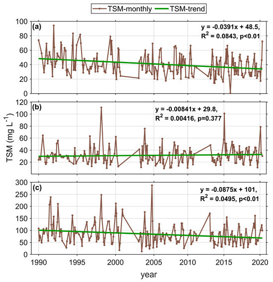
Figure 4.
Interannual variation in TSM concentration during 1990–2020. (a) is for Zone 1 (specific location indicated in Figure 3a, showing a decreasing trend (p < 0.01)); (b) is for Zone 2 (specific location indicated in Figure 3a, showing no apparent linear trend); and (c) is for Zone 3 (specific location indicated in Figure 3a, revealing a decreasing trend (p < 0.01)). Trend analysis is measured in months, with the first month as the starting point. The green lines represent the linear trend.
3.2. Temporal-Spatial Variation in NDVI
Using the GEE, we obtained Landsat Collection 2 Tier 1 L2 Surface Reflectance data for the upper reaches of the Ganges–Brahmaputra delta and the Sundarbans mangrove forest conservation area. The NDVI was calculated for these regions (ROIs indicated in Figure 1b as N1 and N2), and the seasonal average spatial distribution is depicted in Figure 5. In winter, the upstream areas exhibit lower NDVI values, depicted by darker colours in the figure, while the Sundarbans areas show significantly higher NDVI with a distinct boundary. In spring, the high NDVI values in the upstream areas increase, and a noticeable boundary still remains in the Sundarbans mangrove region. In summer, the boundary between the mangrove region and its surrounding areas becomes less distinct as NDVI values converge. In autumn, which marks the end of the rainy season, the NDVI in the study area reaches its annual peak, and NDVI values in most areas are above 0.5, indicating the highest vegetation cover and vigorous plant growth, reaching their peaks in the year.
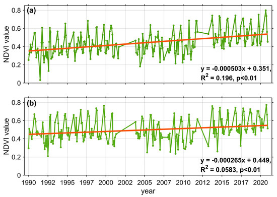
Figure 5.
Temporal distribution of monthly NDVI computed using GEE in the period of 1990–2020. (a) NDVI changes in the upstream delta, with specific locations indicated in Figure 1b N1; (b) NDVI changes in the Sundarbans mangrove reserve area, with specific locations indicated in Figure 1b N2. Both regions exhibit increasing trends (p < 0.01) in NDVI. Trend analysis is measured in months, with the first month as the starting point. The red lines represent the linear trend.
Monthly NDVI data from 1990 to 2020 were computed for the specified regions (N1 and N2) as shown in Figure 1b. Water areas (NDVI < 0) and regions with cloud cover were excluded from the analysis. The arithmetic means of monthly NDVI values for the land portions of N1 and N2 were calculated to obtain a representative NDVI value for the entire area (shown in Figure 5). Comparing the upstream delta region to the mangrove conservation area, the average NDVI values for the former are smaller. Typically, the largest NDVI values occurred from October to November, corresponding to the late stages of the rainy season. Both regions show significant increasing trends (p < 0.01) in NDVI values from 1990 to 2020, indicating an overall improvement in vegetation cover in both the mangrove conservation area and the upstream delta.
3.3. Chlorophyll and Surface Sediment Concentration in the Northern Bay of Bengal
The northern Bay of Bengal is usually regarded as an oligotrophic region, characterised by relatively low chlorophyll and surface sediment concentration. As shown in Figure 6, there is a noticeable increasing trend in chlorophyll (p = 0.10), with the highest value occurring in October 2019, reaching 1.8 mg m−3. Similarly, surface sediment concentration shows an increasing trend (p = 0.09), with its peak appearing in August at 3.1 mg L−1. Both environmental parameters exhibit seasonal variation, generally reaching their highest values in the summer months, and the timings of their peak values are close.
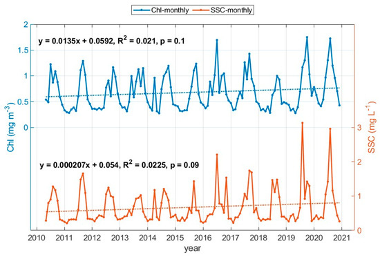
Figure 6.
Monthly variation in MODIS Multi-Sensor Merged Ocean Environmental Parameters from 2010 to 2020. The ROI for the product is detailed in Figure 1b MODIS-ROI. The blue line represents the temporal change in chlorophyll concentration (Chl), showing an increasing trend (p = 0.10); the red line depicts the temporal change in suspended sediment concentration (SSC), which also exhibits an increasing trend (p = 0.09). Trend analysis is measured in months, with the first month as the starting point.
4. Discussion
4.1. Satellite-Derived TSM in the Ganges–Brahmaputra Estuary
For high-turbidity coastal waters, the choice of an appropriate atmospheric correction algorithm can significantly impact data stability and retrieval accuracy. In a field study, Tilstone et al. (2011) [18] conducted TSM measurements at 68 sampling sites in the Ganges–Brahmaputra estuary (approximately 87–89°E, 21–21.5°N) between January 2000 and March 2002. They observed TSM values ranging from 10 to 260 mg L−1, with the majority falling within 25–30 mg L−1. Das et al. (2017) [79] conducted measurements at nine sites in the region of approximately 88.1–88.3°E, 21.1–21.5°N from February 2015 to January 2016, reporting average TSM values ranging from 10 to 50 mg L−1, decreasing from north to south. Patel et al. (2023) [80] conducted TSM sampling at 53 sites within 80.2–81.0°E, 13.0–15.75°N in October 2022, showing TSM values ranging 0–12 mg L−1. Chacko and Jayaram (2017) [81] utilised the MERIS-TSM product spanning from 2002 to 2011; they found that TSM decreased from nearshore waters (>25 mg L−1) to offshore waters (<10 mg L−1), with a substantial spread of high TSM concentration water in the Meghna River estuary. The outcomes obtained through the atmospheric correction algorithm employed in this study align with the results from those aforementioned studies.
The TSM remote sensing inversion results were validated with the in situ measurements. Due to the scarcity of in situ measurements, only 122 sample points from 2009 to 2019 reported from the previous literature [75,82,83,84,85,86,87,88] were selected. As the TSM measurements were often not conducted for satellite validation purposes, the transit times of satellites and the times of in situ observations used for comparison cannot be perfectly matched. Data measured within the same month were selected for validation. The inversion results are generally consistent with the field measurements (see Figure 7). The RMSE between the two datasets is 51.42 mg L–1, the median absolute error (MedianAE) is 22.34 mg L–1, and the determination coefficient (R2) is 0.46 (p < 0.0001). The error in TSM remote sensing inversion falls within an acceptable range, and 30 m resolution Landsat data allow for better characterisation of the spatial distribution of TSM. Therefore, the atmospheric correction algorithm utilised in this study is suitable for high-turbidity waters in the vicinity of the Ganges–Brahmaputra estuary. At the boundaries of the images, the distortion of images arises from the large angle and weak signals received by the sensor, which is reflected in the edges of TSM inversion results. With higher image resolution, signals received by individual photosensitive elements become weaker, making this feature more pronounced, especially for high-resolution sensors. If remote sensing images undergo image mosaicking, it alters the spectral values at the image overlap, adversely affecting TSM inversion. Therefore, we refrain from image mosaicking, presenting the inversion results for each path and row separately.
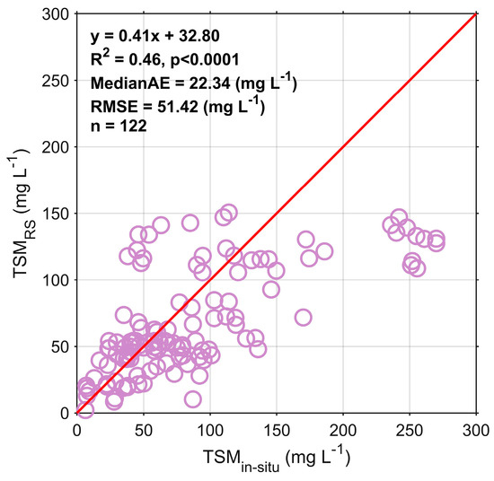
Figure 7.
Comparation of TSM remote sensing inversion (TSMRS) and in situ measurement [75,82,83,84,85,86,87,88] (TSMin-situ). The red line represents the 1:1 relation.
To further validate the accuracy of our results, we compared the TSM values obtained using the atmospheric correction algorithm with the TSM products created by Landsat official atmospheric correction algorithms. We utilised Landsat satellite Collection 2 Tier 1 L2 Surface Reflectance data from the GEE and applied the same inversion algorithm to calculate TSM (see Figure 8). Landsat 5 data were processed using the LEDAPS algorithm [69], while Landsat 8 data were processed using the LaSRC algorithm [70], both of which are based on the 6S model (6S-AC) atmospheric correction algorithm. However, these algorithms primarily rely on the visible and near-infrared (VIR/NIR) spectral bands. Due to the strong scattering effect of suspended particles, the water-leaving radiance in VIR/NIR bands is significantly affected [67,68]. We computed monthly averaged TSM for the three zones (indicated in Figure 3a) and generated corresponding images (Figure 8). The TSM values calculated using the GEE often exhibit extremely high values, ranging from 1000 to 10,000 mg L−1, significantly deviating from the truth. Even when excluding these extremely high outliers, we still find that the GEE TSM results are consistently overestimated across all marine areas and do not exhibit distinct spatial variation, which is not in line with the actual conditions in the study area. This discrepancy can be attributed to the strong reflectance of VIR/NIR bands caused by the high turbidity of the water bodies. As depicted in Figure 8, the GEE provides fewer image points and yields fewer valid data points in comparison with the atmospheric correction used in this study. Additionally, the available data are limited before 2012 (Landsat 5 era), while there was an increase in the volume of available data after 2013 when Landsat 8 was in orbit. The atmospheric correction method employed in this study allowed for more satellite data to be retrieved, offering a more even temporal data distribution and demonstrating superior stability and reliability.
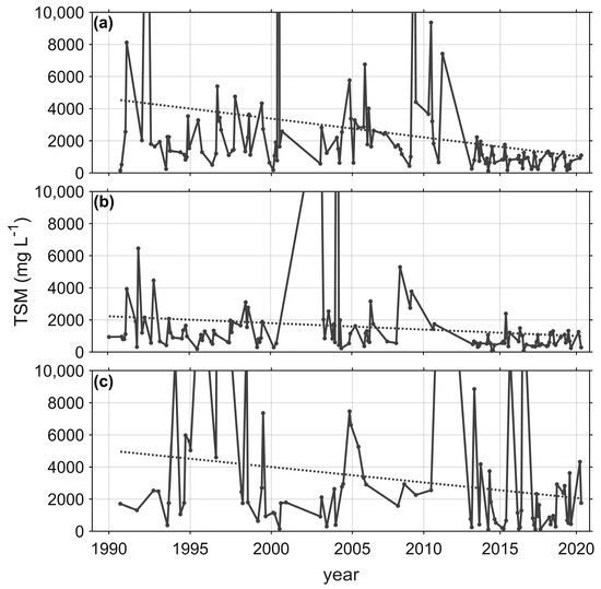
Figure 8.
Interannual variation in TSM concentration from GEE (only displaying values 0–10,000) during 1990–2020. (a) is for Zone 1 (specific location indicated in Figure 3a); (b) is for Zone 2 (specific location indicated in Figure 3a); and (c) is for Zone 3 (specific location indicated in Figure 3a). All show decreasing trends (p < 0.01) in TSM.
4.2. Effects of Hydrology on TSM in the Ganges–Brahmaputra Estuary
We assessed the changes in river discharge along the estuarine sections of the main inflowing rivers of the Ganges–Brahmaputra delta using the GloFAS discharge data. Annual average discharge variation in the wet season and dry season are shown in Figure 9a–d. In the downstream region of the Ganges River, the primary tributaries exhibit significantly different magnitudes of discharge, ranging from 103 to 105 m3 s−1. The order of discharge magnitude from the smallest to the largest is the Baleswar River, Hooghly River, and Meghna River. Section S1 (Figure 9a) spans the Hooghly River, and exhibits a higher discharge with an annual average of approximately 1500 m3 s−1. Section S2 and S3 span the Baleswar River (Figure 9b,c), which flows through the mangrove areas where the presence of vegetation leads to reduced discharge, resulting in annual average discharge below 1000 m3 s−1. Section S4 (Figure 9d), spanning the Meghna River, represents the largest tributary in terms of discharge, with an annual average of about 50,000 m3 s−1. The Ganges–Brahmaputra delta experiences distinct dry and wet seasons, with the wet season typically starting in May or June and extending through October or November. The discharge trends of most sections are not significant, except for a slight decrease in the wet season in S3 (p < 0.05).
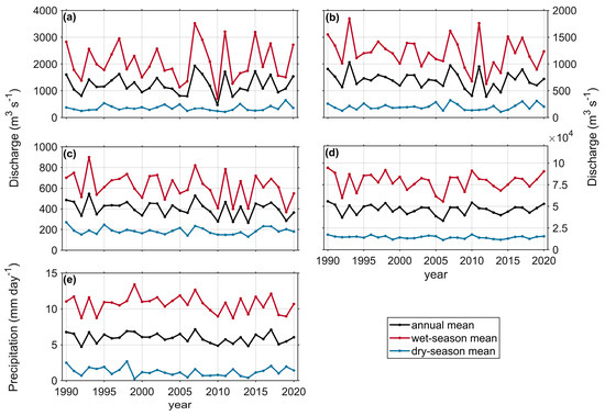
Figure 9.
Time series of discharge and precipitation in the period 1990–2020. (a–d) Interannual variation in discharge for sections S1–S4 (locations detailed in Figure 1b). (e) Interannual variation in precipitation, covering the region outlined in Figure 1b. The black line represents annual average data; the red line, wet season data; and the blue line, dry season data.
Using monthly average precipitation data from the GPCP, we calculated the mean precipitation for the downstream Ganges–Brahmaputra delta (refer to Pr in Figure 1b) to represent the precipitation characteristics of the entire study area (see Figure 9e). The annual mean precipitation in the study area fluctuates between 4.79 and 6.80 mm day−1, with the maximum and minimum annual precipitation occurring in 2007 and 2010, respectively. Similar to the seasonal variation in discharge, the precipitation in the Ganges–Brahmaputra delta exhibits distinct seasonal patterns, with more precipitation occurring from May to October, and less precipitation for the rest of the year. Examining the time series, we see no significant trend in precipitation over time.
The precipitation and river discharge of the basin can influence estuary TSM from erosion and resuspension perspectives. The magnitude of precipitation and river discharge reflects the strength of hydrodynamic conditions, thus affecting land erosion. When hydrodynamics is strong, rivers have a higher capacity for land erosion, leading to increased TSM as they transport additional sediment. Conversely, when the hydrodynamics are weak, rivers have a lower sediment-carrying capacity, which is not conducive to sediment transport. Halder and Chowdhury (2023) [89] used long-term remote sensing data to study the morphological changes of the Padma River in central Bangladesh, and found a strong linear relationship between erosion and discharge during high-flow periods (R2 = 0.9989). Rivers bring freshwater to the bay, and the larger the river discharge, the lower the salinity in the bay. This condition is unfavourable for the sediment coagulation process [37], leading to a broader dispersion of regions with higher TSM concentration. Both of these processes have the same directional effect on TSM. Therefore, TSM concentration is notably increased during the summer and autumn when river discharge and precipitation are higher, and areas with high TSM have a broader water coverage.
Both precipitation and river discharge exhibit interannual fluctuations. However, no significant trend was found during the study period for either one. According to Li et al. (2020) [16], the hydrological characteristics of the Ganges–Brahmaputra River system can be classified as Pattern II (S-D), where river discharge remains relatively stable while the output of suspended sediment decreases. In this context, river discharge could not be the dominant factor influencing the TSM long-term trend. Zheng et al. (2021) [90] conducted a long-term analysis of discharge and suspended sediment concentration in the Padma River (the upper reach of the Meghna River) from 1990 to 2019, and found that the suspended sediment flux in this area was significantly reduced (p < 0.01). They also found a certain correlation between discharge change and suspended sediment export (R = 0.44, p < 0.05). Since the suspended sediment output flux is the product of flow and TSM, it can be inferred that TSM decreased where river discharge did not change significantly. Rahman et al. (2018) [6] used hydrological models to investigate changes in the total water and suspended sediment flux in the Ganges–Brahmaputra River basin from 1958 to 2008. They observed that, for the Ganges, the rate of decrease in sediment load significantly exceeded that of water discharge, whereas for the Brahmaputra, its total water volume did not change significantly, but its sediment load decreased. In summary, changes in hydrological elements are crucial factors affecting the seasonal distribution pattern of TSM. However, long-term changes in river discharge and precipitation cannot explain the gradual decrease in TSM over the recent three decades in this paper.
The spatial distribution of TSM in the study area is influenced not only by river discharge but also by tidal currents and wave action [91,92]. In the nearshore regions of the northern Bay of Bengal, tides exert a significant influence during a considerable portion of the period [44]. However, during the monsoon season (a period of high flow rates), the impact of tides noticeably diminishes [93]. Furthermore, wind waves may contribute to the resuspension of TSM [94]. During the monsoon season from June to September, the prevailing southwest monsoon in the region often gives rise to intense storm events [44]. This phenomenon affects a substantial part of the Indian subcontinent, with wave activities superimposed on tidal currents. The combined effect is capable of resuspending bottom sediments in water depths less than 10 m [95]. Consequently, this resuspension makes it more challenging for suspended sediments to settle, resulting in higher concentration of nearshore TSM during summer and autumn. The southwest monsoon also drives water from the open sea toward the land, causing the turbidity maximum to concentrate more toward the shore. This tendency is particularly evident in the summer TSM distribution in the Hooghly River estuary. The turbidity maximum in the Hooghly River estuary is predominantly confined to the river channel, aligning with the MERIS-TSM inversion of Chacko and Jayaram (2017) [81].
Phenomena such as the El Niño–Southern Oscillation (ENSO) and the Indian Ocean Dipole (IOD) can influence sea surface temperatures in this region, impacting the pattern and intensity of the monsoon [96]. These events significantly affect precipitation and discharge in the northern Bay of Bengal and its coastal area, leading to major floods in some years such as 1998, 2007, and 2011 [97]. Intense seasonal or event-scale precipitation can increase river sediment discharge [98], thereby elevating nearshore TSM. Some studies at the geological scale, based on sedimentary records [99,100,101], also suggested that stronger monsoons result in increased sediment supply from rivers to the northern Bay of Bengal. However, it is difficult to distinguish TSM interannual variation caused by monsoonal variation as the relationship among monsoon, precipitation, and river discharge are linked. Therefore, for a more accurate understanding and discussion of the relationship between monsoonal interannual variation and TSM, it is more suitable to integrate numerical models.
4.3. Land-Use Change and Its Effects on TSM in Estuaries
TSM in water is a primary factor in maintaining sedimentation rates in deltas [102]. Prolonged and excessive reductions in water sediment concentration may have potential negative effects on local ecosystem functions. Changes in land use can affect a river’s erosion capacity on soil, thus altering the concentration of suspended particles in the water. Figure 4 shows that TSM in Zone 2 has no clear trend over the 31 years and had relatively low fluctuations. In contrast, the other two areas experience significant decreases in TSM. Goswami et al. (2023) [103] analysed a 15 km buffer zone of the Hooghly River and found that the predominant land-use type was agricultural land, constituting 56.7–67% (without water bodies), and the downstream of the Hooghly River exhibit strong hydraulic conditions due to the meandering nature of the riverbanks and tidal effects. Hoque et al. (2020) [104] conducted a similar study on land use downstream of the Meghna River, where agricultural land accounted for 38.07–48.68% of the total land use (including water bodies, ranging from 26.44% to 26.15%). This region also experienced high-intensity hydraulic activities and had a high rate of erosion [105]. Consequently, these factors contribute to the elevated and fluctuating TSM concentration in these two river estuaries. In contrast, the Sundarbans mangrove forest has maintained a consistent area from 1980 to 2020, covering over 50% (including water bodies, ranging from 26.48% to 32.93%) [106]. Furthermore, mangroves have evolved strong root systems to adapt to the complexities of coastal environments [107]. These roots enhance friction and reduce tidal flow velocities, allowing them to capture and aggregate sediments [108], which helps stabilise TSM concentration downstream in the bay. Dunn et al. (2018) [109] conducted a study by introducing upstream dam construction into a global hydrological model to analyse the factors influencing suspended sediment flux in the Ganges–Brahmaputra River system since the 21st century. They employed various scenario simulations (including scenarios with no anthropogenic disturbances, current conditions, and potential future changes, among 12 possible scenarios). They found that in the absence of anthropogenic disturbances, the annual suspended sediment flux is the highest, whereas introducing anthropogenic factors resulted in the lowest suspended sediment flux. This suggests that the primary reason for reduced sediment flux is direct anthropogenic interference within the river basin rather than global climate change.
In practical research, the NDVI has been widely used as a representative of land vegetation productivity and as an indicator of overall mangrove health [110]. In this study, we calculated the monthly average NDVI of the entire Ganges–Brahmaputra delta upstream area and the monthly average NDVI of the Sundarbans mangrove reserve area. The NDVI of the two areas showed a significant upward trend (p < 0.01), indicating that the watershed vegetation and mangroves are well maintained.
Previous studies showed that the mangrove area increased in the recent years [111,112,113], which can be attributed to a series of environmental protection agreements signed by India and Bangladesh in 2014 [113] and initiated collaborations in the blue economy, implementing environmental conservation measures. These efforts included the construction of the Farakka Barrage on the Ganges to ensure a fresh water supply to the Sundarbans region [114]. The implementation of these measures has played a role in enhancing the NDVI of the Ganges–Brahmaputra delta and preserving its ecosystems. Zheng et al. (2021) [90] used the MODIS global monthly NDVI product and Landsat data to obtain monthly average NDVI images for the Padma River basin, which includes the ROI used for the NDVI in this study, covering the period from 2000 to 2019. They found an upward trend in NDVI, indicating an increase in vegetation cover in the Ganges–Brahmaputra basin. This increase in vegetation cover enhances the land’s resistance to runoff erosion, slowing down soil erosion, and consequently reducing the concentration of TSM in the water. Urbanisation in the Ganges–Brahmaputra delta is ongoing. Inevitably, protective measures are being implemented along the shoreline (e.g., Crawford et al. (2020) [115]), and in various projects such as embankment reinforcement taking place in parts of India [116], reducing erosion of the riverbanks. These actions contribute to a decreasing trend in TSM, aligning with our results in this study.
4.4. Chlorophyll and Surface Sediment Concentration Variation in the Northern Bay of Bengal
Owing to the inflow of the Ganges–Brahmaputra River system of freshwater and terrestrial materials, the northern Bay of Bengal constitutes a river–estuary–coastal sea continuum system. Researchers have regarded this region as an excellent area for the study of marine environments [117,118]. Due to the interaction of various factors, such as the reversal of monsoon winds and the superimposition of planetary waves [119], the northern Bay of Bengal has developed a unique circulation system. It exhibits cyclonic circulation characteristics during winter and anticyclonic circulation characteristics during summer. The seasonally reversing monsoons and resulting circulation patterns have profound impacts on the biogeochemical characteristics of this region [120]. Under the combined influence of these factors, the water quality parameters in the northern bay also exhibit distinct seasonal variation. The combined effect of these factors leads to significant seasonal variation in water quality parameters.
Surface sediment concentration and chlorophyll are two important water quality parameters and are known to interact with each other. On the one hand, the input of suspended sediments provides nutrients and attachment sites for marine microorganisms, promoting local primary productivity [121]. On the other hand, marine organisms in their life cycles produce a substantial amount of suspended matter [18], which can be resuspend into the water. Surface sediment concentration and chlorophyll in the northern Bay of Bengal (20–21°N), both peaks in summer, as shown in Figure 6. Chacko and Jayaram (2017) [81] analysed monthly MERIS data for the region between 87°E and 92°E and between 17°N and 23°N (partially overlapping our study area, as shown in Figure 1b); also of note are that areas with high TSM concentration were typically situated north of 21.5°N, but during the summer monsoon period, high TSM water extended southward to 20°N. Tilstone et al. (2011) [18] used monthly SeaWiFS chlorophyll data from 1998 to 2007 and found that chlorophyll along the coastal regions of the Bay of Bengal peaked 1–2 months after the peak river flow periods. This phenomenon results from a combination of factors, including river nutrient enrichment, tidal mixing, and eddy interactions [122].
From 1990 to 2020, the river discharge in the area did not exhibit a significant trend, indicating that the input of freshwater into the northern bay had not changed dramatically over this extended period. However, the TSM levels had been consistently decreasing. Interestingly, the trends in chlorophyll and surface sediment concentration of the northern Bay of Bengal during 2010–2020 both show slight increases. Some studies [123,124] suggested that due to the narrow continental shelf in the northern Bay of Bengal, nutrients brought by rivers are transported by ocean currents into deeper areas of the water column, where they may not be fully accessible to surface marine biota. The long-term influence of the river system on the northern Bay of Bengal is primarily related to the input of freshwater and dissolved nutrients. However, the sediment reduction weakened this impact, attributed to improvements in local land management, coastal protection measures, dam construction, and an increase in vegetation cover. In summary, because the summer monsoon brings the majority of annual river discharge, the land-sourced input significantly influences the water quality in the Bay of Bengal on a seasonal time scale. However, it seems that the long-term changes of surface sediment concentration and chlorophyll in the northern Bay of Bengal are not dominated by terrestrial inputs. A possible reason may be related to the change in wind stress, mesoscale processes, etc., but those are out the scope of this study.
5. Conclusions
In this study, we utilised an atmospheric correction algorithm based on the general exact Rayleigh scattering look-up-table and SWIR band extrapolation to obtain accurate Landsat 8 (OLI/TIRS) L1 products and Landsat 5 (TM) L1 radiance information for the Ganges–Brahmaputra estuary region from 1990 to 2020. Then, we conducted inversion to derive a long-term, high-precision time series of TSM for the study area. We analysed seasonal and interannual variation in water TSM in the Ganges–Brahmaputra estuary by considering local parameters such as vegetation cover, discharge, and precipitation. We also investigated the impact of terrestrial input on the marine ecosystem by integrating data from the northern Bay of Bengal, specifically the surface sediment concentration and chlorophyll products. We examined the environmental changes across the entire river–estuary–coast continuum and provided valuable insights into the long-term environmental dynamics of this area.
We obtained the 30-year time series of sediment concentration in the Ganges–Brahmaputra estuary. In terms of spatial distribution, TSM in the Ganges–Brahmaputra estuary decreases from the river mouth toward the open sea, with the maximum turbidity zone appearing either at the river mouth or at the bay head depending on the intensity of the discharge and monsoon. TSM concentration in these areas typically exceed 100 mg L−1. The TSM displays prominent seasonal variation; the TSM in summer and autumn during the wet season is significantly higher than that in winter and spring. Such variation is closely linked to seasonal changes in precipitation and river discharge. Over the long-term scale of more than 30 years, the TSM in the estuary exhibits a fluctuating decreasing trend, which is mainly attributed to land-use changes and anthropogenic activities rather than river discharge and precipitation.
Using data from surface sediment concentration and chlorophyll products from 2010 to 2020 in the northern Bay of Bengal, we examined the impact of terrestrial inputs on the local marine ecosystem. Surface sediment concentration and chlorophyll data exhibit similar trends over the 10 years, showing slight increases with noticeable seasonal fluctuations. Due to the major influx of discharge during the summer monsoon, terrestrial inputs have a relatively more significant impact on the seasonal-scale water quality in the northern bay. However, the long-term influence of terrestrial inputs on surface sediment concentration and chlorophyll in the northern bay is limited.
The results of this study underscore the environmental challenges faced by the Ganges–Brahmaputra estuary, particularly the reduced supply of delta sediments due to human activities. Sustainable management in the future will need to take these factors into account to ensure the environmental health and socio-economic development of the region. In developing countries such as Bangladesh, while there are some flow monitoring and sediment sampling stations, many sites operate only for limited periods during the year [109], resulting in poor data quality and a lack of temporal continuity in water–sediment data. This study provides a reference example for developing countries lacking in situ data for research on sediment transport.
Author Contributions
Conceptualization, X.C.; methodology, X.C. and H.Y.; software, H.Y. and T.M.; validation, H.Y., X.C. and T.M.; formal analysis and investigation, T.M. and H.Y.; resources, X.C.; data curation, T.M. and H.Y.; writing—original draft preparation, H.Y. and T.M.; writing—review and editing, X.C.; visualization, H.Y. and T.M.; supervision, X.C.; funding acquisition, X.C. All authors have read and agreed to the published version of the manuscript.
Funding
This study was supported by the National Key Research and Development Program of China (Grants #2022YFC3104900 and #2022YFC3104903) and the National Natural Science Foundation of China (Grants #42176177, #42006165, and #41825014).
Data Availability Statement
The raw data supporting the conclusions of this article will be made available by the authors on request.
Acknowledgments
This work is based on Mei’s summer internship project at SOED/SIO during 2022–2023. We would like to thank the USGS for the Landsat data. We also thank the satellite ground station and the satellite data processing and sharing centre of SOED/SIO for help with data processing. We thank the editors and reviewers for their careful work and thoughtful suggestions.
Conflicts of Interest
The authors declare no conflicts of interest.
References
- Goodbred, S., Jr.; Kuehl, S.A. The significance of large sediment supply, active tectonism, and eustasy on margin sequence development: Late Quaternary stratigraphy and evolution of the Ganges–Brahmaputra delta. Sediment. Geol. 2000, 133, 227–248. [Google Scholar] [CrossRef]
- Goodbred, S.L., Jr.; Kuehl, S.A. Enormous Ganges-Brahmaputra sediment discharge during strengthened early Holocene monsoon. Geology 2000, 28, 1083–1086. [Google Scholar] [CrossRef]
- Akter, J.; Sarker, M.H.; Popescu, I.; Roelvink, D. Evolution of the Bengal Delta and its prevailing processes. J. Coast. Res. 2016, 32, 1212–1226. [Google Scholar] [CrossRef]
- Chowdary, J.; John, N.; Gnanaseelan, C. Interannual variability of surface air-temperature over India: Impact of ENSO and Indian Ocean Sea surface temperature. Int. J. Climatol. 2014, 34, 416–429. [Google Scholar] [CrossRef]
- Steckler, M.S.; Nooner, S.L.; Akhter, S.H.; Chowdhury, S.K.; Bettadpur, S.; Seeber, L.; Kogan, M.G. Modeling Earth deformation from monsoonal flooding in Bangladesh using hydrographic, GPS, and Gravity Recovery and Climate Experiment (GRACE) data. J. Geophys. Res. Solid Earth 2010, 115, B08407. [Google Scholar] [CrossRef]
- Rahman, M.; Dustegir, M.; Karim, R.; Haque, A.; Nicholls, R.J.; Darby, S.E.; Nakagawa, H.; Hossain, M.; Dunn, F.E.; Akter, M. Recent sediment flux to the Ganges-Brahmaputra-Meghna delta system. Sci. Total Environ. 2018, 643, 1054–1064. [Google Scholar] [CrossRef] [PubMed]
- Rudra, K. Changing river courses in the western part of the Ganga–Brahmaputra delta. Geomorphology 2014, 227, 87–100. [Google Scholar] [CrossRef]
- Wang, Y.-H.; Deng, A.-J.; Feng, H.-C.; Wang, D.-W.; Guo, C.-S. Tide-modulated river discharge division in the Ganges-Brahmaputra-Meghna delta channel network, Bangladesh. J. Hydrol. Reg. Stud. 2023, 49, 101493. [Google Scholar] [CrossRef]
- Konkol, A.; Schwenk, J.; Katifori, E.; Shaw, J.B. Interplay of river and tidal forcings promotes loops in coastal channel networks. Geophys. Res. Lett. 2022, 49, e2022GL098284. [Google Scholar] [CrossRef]
- Yan, Z.; Tang, D. Changes in suspended sediments associated with 2004 Indian Ocean tsunami. Adv. Space Res. 2009, 43, 89–95. [Google Scholar] [CrossRef]
- Nicholls, R.J.; Goodbred, S. Towards integrated assessment of the Ganges-Brahmaputra Delta. In Proceedings of the 5th International Conference on Asian Marine Geology, and 1st Annual Meeting of IGCP475 DeltaMAP and APN Mega-Deltas, Bangkok, Thailand, 13–18 January 2004; p. 9. [Google Scholar]
- Paszkowski, A.; Goodbred Jr, S.; Borgomeo, E.; Khan, M.S.A.; Hall, J.W. Geomorphic change in the Ganges–Brahmaputra–Meghna delta. Nat. Rev. Earth Environ. 2021, 2, 763–780. [Google Scholar] [CrossRef]
- Islam, N. Environmental Challenges to Bangladesh; Bangladesh Institute of International and Strategic Studies: Dhaka, Bangladesh, 1991. [Google Scholar]
- Jarriel, T.; Isikdogan, L.F.; Bovik, A.; Passalacqua, P. System wide channel network analysis reveals hotspots of morphological change in anthropogenically modified regions of the Ganges Delta. Sci. Rep. 2020, 10, 12823. [Google Scholar] [CrossRef] [PubMed]
- Giri, C.; Long, J.; Abbas, S.; Murali, R.M.; Qamer, F.M.; Pengra, B.; Thau, D. Distribution and dynamics of mangrove forests of South Asia. J. Environ. Manag. 2015, 148, 101–111. [Google Scholar] [CrossRef]
- Li, L.; Ni, J.; Chang, F.; Yue, Y.; Frolova, N.; Magritsky, D.; Borthwick, A.G.L.; Ciais, P.; Wang, Y.; Zheng, C.; et al. Global trends in water and sediment fluxes of the world’s large rivers. Sci. Bull. 2020, 65, 62–69. [Google Scholar] [CrossRef] [PubMed]
- Aziz, A.; Paul, A.R. Bangladesh Sundarbans: Present Status of the Environment and Biota. Diversity 2015, 7, 242–269. [Google Scholar] [CrossRef]
- Tilstone, G.H.; Angel-Benavides, I.M.; Pradhan, Y.; Shutler, J.D.; Groom, S.; Sathyendranath, S. An assessment of chlorophyll-a algorithms available for SeaWiFS in coastal and open areas of the Bay of Bengal and Arabian Sea. Remote Sens. Environ. 2011, 115, 2277–2291. [Google Scholar] [CrossRef]
- Ilyina, T.; Pohlmann, T.; Lammel, G.; Sündermann, J. A fate and transport ocean model for persistent organic pollutants and its application to the North Sea. J. Mar. Syst. 2006, 63, 1–19. [Google Scholar] [CrossRef]
- Mayer, L.M.; Keil, R.G.; Macko, S.A.; Joye, S.B.; Ruttenberg, K.C.; Aller, R.C. Importance of suspended participates in riverine delivery of bioavailable nitrogen to coastal zones. Glob. Biogeochem. Cycles 1998, 12, 573–579. [Google Scholar] [CrossRef]
- Webster, T.; Lemckert, C. Sediment resuspension within a microtidal estuary/embayment and the implication to channel management. J. Coast. Res. 2002, 36, 753–759. [Google Scholar] [CrossRef]
- Sathyendranath, S.; Gouveia, A.D.; Shetye, S.R.; Ravindran, P.; Platt, T. Biological control of surface temperature in the Arabian Sea. Nature 1991, 349, 54–56. [Google Scholar] [CrossRef]
- Sarmiento, J.L.; Hughes, T.M.; Stouffer, R.J.; Manabe, S. Simulated response of the ocean carbon cycle to anthropogenic climate warming. Nature 1998, 393, 245–249. [Google Scholar] [CrossRef]
- Field, C.B.; Behrenfeld, M.J.; Randerson, J.T.; Falkowski, P. Primary production of the biosphere: Integrating terrestrial and oceanic components. Science 1998, 281, 237–240. [Google Scholar] [CrossRef] [PubMed]
- Cornell, S.; Randell, A.; Jickells, T. Atmospheric inputs of dissolved organic nitrogen to the oceans. Nature 1995, 376, 243–246. [Google Scholar] [CrossRef]
- Abbas, N.; Subramanian, V. Erosion and sediment transport in the Ganges river basin (India). J. Hydrol. 1984, 69, 173–182. [Google Scholar] [CrossRef]
- Jha, P.K.; Subramanian, V.; Sitasawad, R. Chemical and sediment mass transfer in the Yamuna River—A tributary of the Ganges system. J. Hydrol. 1988, 104, 237–246. [Google Scholar] [CrossRef]
- Barua, D.K. Suspended sediment movement in the estuary of the Ganges-Brahmaputra-Meghna river system. Mar. Geol. 1990, 91, 243–253. [Google Scholar] [CrossRef]
- Gain, A.K.; Rahman, M.M.; Sadik, M.S.; Adnan, M.S.G.; Ahmad, S.; Ahsan, S.M.M.; Ashik-Ur-Rahman, M.; Balke, T.; Datta, D.K.; Dewan, C.; et al. Overcoming challenges for implementing nature-based solutions in deltaic environments. Insights Ganges-Brahmaputra Delta Bangladesh 2022, 17, 064052. [Google Scholar] [CrossRef]
- Mckim, H.L.; Merry, C.J.; Layman, R. Water quality monitoring using an airborne spectroradiometer. Photogramm. Eng. Remote Sens. 1984, 50, 353–360. [Google Scholar]
- Curran, P.; Wilkinson, W. Mapping the concentration and dispersion of dye from a long sea outfall using digitized aerial photography. Int. J. Remote Sens. 1985, 6, 1735–1748. [Google Scholar] [CrossRef]
- Nishat, B.; Rahman, S.M.M. Water Resources Modeling of the Ganges-Brahmaputra-Meghna River Basins Using Satellite Remote Sensing Data1. JAWRA J. Am. Water Resour. Assoc. 2009, 45, 1313–1327. [Google Scholar] [CrossRef]
- Zhou, W.; Wang, S.; Zhou, Y.; Troy, A. Mapping the concentrations of total suspended matter in Lake Taihu, China, using Landsat-5 TM data. Int. J. Remote Sens. 2006, 27, 1177–1191. [Google Scholar] [CrossRef]
- Wang, F.; Zhou, B.; Liu, X.; Zhou, G.; Zhao, K. Remote-sensing inversion model of surface water suspended sediment concentration based on in situ measured spectrum in Hangzhou Bay, China. Environ. Earth Sci. 2012, 67, 1669–1677. [Google Scholar] [CrossRef]
- Qiu, Z. A simple optical model to estimate suspended particulate matter in Yellow River Estuary. Opt. Express 2013, 21, 27891–27904. [Google Scholar] [CrossRef] [PubMed]
- Doxaran, D.; Cherukuru, N.; Lavender, S.J. Apparent and inherent optical properties of turbid estuarine waters: Measurements, empirical quantification relationships, and modeling. Appl. Opt. 2006, 45, 2310–2324. [Google Scholar] [CrossRef]
- Islam, M.R.; Yamaguchi, Y.; Ogawa, K. Suspended sediment in the Ganges and Brahmaputra Rivers in Bangladesh: Observation from TM and AVHRR data. Hydrol. Process. 2001, 15, 493–509. [Google Scholar] [CrossRef]
- Nechad, B.; Alvera-Azcaràte, A.; Ruddick, K.; Greenwood, N. Reconstruction of MODIS total suspended matter time series maps by DINEOF and validation with autonomous platform data. Ocean Dyn. 2011, 61, 1205–1214. [Google Scholar] [CrossRef]
- Duane Nellis, M.; Harrington, J.A.; Wu, J. Remote sensing of temporal and spatial variations in pool size, suspended sediment, turbidity, and Secchi depth in Tuttle Creek Reservoir, Kansas: 1993. Geomorphology 1998, 21, 281–293. [Google Scholar] [CrossRef]
- Miller, R.L.; McKee, B.A. Using MODIS Terra 250 m imagery to map concentrations of total suspended matter in coastal waters. Remote Sens. Environ. 2004, 93, 259–266. [Google Scholar] [CrossRef]
- Shi, W.; Wang, M. Satellite observations of flood-driven Mississippi River plume in the spring of 2008. Geophys. Res. Lett. 2009, 36. [Google Scholar] [CrossRef]
- Pandey, P.; Kunte, P.D. Geospatial approach towards enumerative analysis of suspended sediment concentration for Ganges–Brahmaputra Bay. Comput. Geosci. 2016, 95, 32–58. [Google Scholar] [CrossRef]
- Cai, L.; Tang, D.; Li, C. An investigation of spatial variation of suspended sediment concentration induced by a bay bridge based on Landsat TM and OLI data. Adv. Space Res. 2015, 56, 293–303. [Google Scholar] [CrossRef]
- Islam, M.R.; Begum, S.F.; Yamaguchi, Y.; Ogawa, K. Distribution of suspended sediment in the coastal sea off the Ganges–Brahmaputra River mouth: Observation from TM data. J. Mar. Syst. 2002, 32, 307–321. [Google Scholar] [CrossRef]
- Sahoo, D.P.; Sahoo, B.; Tiwari, M.K. MODIS-Landsat fusion-based single-band algorithms for TSS and turbidity estimation in an urban-waste-dominated river reach. Water Res. 2022, 224, 119082. [Google Scholar] [CrossRef]
- Islam, M.S. Perspectives of the coastal and marine fisheries of the Bay of Bengal, Bangladesh. Ocean Coast. Manag. 2003, 46, 763–796. [Google Scholar] [CrossRef]
- Joy, M.A.R.; Upaul, S.; Fatema, K.; Amin, F.M.R. Application of GIS and remote sensing in morphometric analysis of river basin at the south-western part of great Ganges delta, Bangladesh. Hydrol. Res. 2023, 54, 739–755. [Google Scholar] [CrossRef]
- Khandu; Awange, J.L.; Kuhn, M.; Anyah, R.; Forootan, E. Changes and variability of precipitation and temperature in the Ganges-Brahmaputra-Meghna River Basin based on global high-resolution reanalyses. Int. J. Climatol. 2017, 37, 2141–2159. [Google Scholar] [CrossRef]
- Chowdhury, M.R.; Ward, N. Hydro-meteorological variability in the greater Ganges–Brahmaputra–Meghna basins. Int. J. Climatol. A J. R. Meteorol. Soc. 2004, 24, 1495–1508. [Google Scholar] [CrossRef]
- Chowdhury, M.R. Flood monitoring in Bangladesh: Experience from normal and catastrophic floods. J. Jpn. Assoc. Hydrol. Sci. 1996, 26, 241–252. [Google Scholar]
- U.S. Geological Survey. Available online: https://earthexplorer.usgs.gov/ (accessed on 4 September 2022).
- Collection 2 Tiers. Available online: https://www.usgs.gov/core-science-systems/nli/landsat/landsat-collection-2?qt-science_support_page_related_con=1#qt-science_support_page_related_con. (accessed on 7 September 2023).
- SatCO2. Available online: https://www.satco2.com/ (accessed on 30 August 2023).
- He, X.; Bai, Y.; Pan, D.; Zhu, Q. The atmospheric correction algorithm for HY-1B/COCTS. In Proceedings of the Geoinformatics 2008 and Joint Conference on GIS and Built Environment: Classification of Remote Sensing Images, Guangzhou, China, 28–29 June 2008; pp. 387–398. [Google Scholar]
- Bai, Y.; Jiang, L.; He, X.; Barale, V. An Introduction to Optical Remote Sensing of the Asian Seas: Chinese Dedicated Satellites and Data Processing Techniques. In Remote Sensing of the Asian Seas; Barale, V., Gade, M., Eds.; Springer International Publishing: Cham, Switzerland, 2019; pp. 61–79. [Google Scholar]
- Tassan, S. An improved in-water algorithm for the determination of chlorophyll and suspended sediment concentration from Thematic Mapper data in coastal waters. Int. J. Remote Sens. 1993, 14, 1221–1229. [Google Scholar] [CrossRef]
- Grimaldi, S.; Salamon, P.; Disperati, J.; Zsoter, E.; Russo, C.; Ramos, A.; Carton De Wiart, C.; Barnard, C.; Hansford, E.; Gomes, G.; et al. River Discharge and Related Historical Data from the Global Flood Awareness System. v4.0. European Commission, Joint Research Centre (JRC). Available online: https://cds.climate.copernicus.eu/cdsapp#!/dataset/cems-glofas-historical (accessed on 17 August 2023).
- GPCP Version 3.2 Satellite-Gauge (SG) Combined Precipitation Data Set. Available online: https://disc.gsfc.nasa.gov/datacollection/GPCPMON_3.2.html (accessed on 17 August 2023).
- Earth Data Search Platform. Available online: https://search.earthdata.nasa.gov/search (accessed on 30 August 2023).
- IOCCG. Atmospheric Correction for Remotely-Sensed Ocean-Colour Products; International Ocean Colour Coordinating Group (IOCCG): Dartmouth, NS, Canada, 2010; Volume 78. [Google Scholar]
- Green, M.O.; Coco, G. Review of wave-driven sediment resuspension and transport in estuaries. Rev. Geophys. 2014, 52, 77–117. [Google Scholar] [CrossRef]
- Pahlevan, N.; Mangin, A.; Balasubramanian, S.V.; Smith, B.; Alikas, K.; Arai, K.; Barbosa, C.; Bélanger, S.; Binding, C.; Bresciani, M.; et al. ACIX-Aqua: A global assessment of atmospheric correction methods for Landsat-8 and Sentinel-2 over lakes, rivers, and coastal waters. Remote Sens. Environ. 2021, 258, 112366. [Google Scholar] [CrossRef]
- Vanhellemont, Q.; Ruddick, K. Advantages of high quality SWIR bands for ocean colour processing: Examples from Landsat-8. Remote Sens. Environ. 2015, 161, 89–106. [Google Scholar] [CrossRef]
- Zhang, Y.; He, X.; Lian, G.; Bai, Y.; Yang, Y.; Gong, F.; Wang, D.; Zhang, Z.; Li, T.; Jin, X. Monitoring and spatial traceability of river water quality using Sentinel-2 satellite images. Sci. Total Environ. 2023, 894, 164862. [Google Scholar] [CrossRef] [PubMed]
- He, X.; Pan, D.; Bai, Y.; Mao, Z.; Gong, F. General exact Rayleigh scattering look-up-table for ocean color remote sensing. Remote Sens. Mar. Environ. 2006, 6406, 319–328. [Google Scholar] [CrossRef]
- He, X.; Bai, Y.; Zhu, Q.; Gong, F. A vector radiative transfer model of coupled ocean–atmosphere system using matrix-operator method for rough sea-surface. J. Quant. Spectrosc. Radiat. Transf. 2010, 111, 1426–1448. [Google Scholar] [CrossRef]
- Wang, M. Remote sensing of the ocean contributions from ultraviolet to near-infrared using the shortwave infrared bands: Simulations. Appl. Opt. 2007, 46, 1535–1547. [Google Scholar] [CrossRef]
- Wang, M.; Shi, W. The NIR-SWIR combined atmospheric correction approach for MODIS ocean color data processing. Opt. Express 2007, 15, 15722–15733. [Google Scholar] [CrossRef]
- Schmidt, G.; Jenkerson, C.B.; Masek, J.; Vermote, E.; Gao, F. Landsat Ecosystem Disturbance Adaptive Processing System (LEDAPS) Algorithm Description; No. 2013-1057; US Geological Survey: Reston, VA, USA, 2013; p. 27. [Google Scholar]
- Vermote, E.; Roger, J.C.; Franch, B.; Skakun, S. LaSRC (Land Surface Reflectance Code): Overview, application and validation using MODIS, VIIRS, LANDSAT and Sentinel 2 data’s. In Proceedings of the IGARSS 2018—2018 IEEE International Geoscience and Remote Sensing Symposium, Valencia, Spain, 22–27 July 2018; pp. 8173–8176. [Google Scholar]
- Nechad, B.; Ruddick, K.G.; Park, Y. Calibration and validation of a generic multisensor algorithm for mapping of total suspended matter in turbid waters. Remote Sens. Environ. 2010, 114, 854–866. [Google Scholar] [CrossRef]
- Dogliotti, A.I.; Ruddick, K.G.; Nechad, B.; Doxaran, D.; Knaeps, E. A single algorithm to retrieve turbidity from remotely-sensed data in all coastal and estuarine waters. Remote Sens. Environ. 2015, 156, 157–168. [Google Scholar] [CrossRef]
- Ciancia, E.; Campanelli, A.; Lacava, T.; Palombo, A.; Pascucci, S.; Pergola, N.; Pignatti, S.; Satriano, V.; Tramutoli, V. Modeling and Multi-Temporal Characterization of Total Suspended Matter by the Combined Use of Sentinel 2-MSI and Landsat 8-OLI Data: The Pertusillo Lake Case Study (Italy). Remote Sens. 2020, 12, 2147. [Google Scholar] [CrossRef]
- Odermatt, D.; Gitelson, A.; Brando, V.E.; Schaepman, M. Review of constituent retrieval in optically deep and complex waters from satellite imagery. Remote Sens. Environ. 2012, 118, 116–126. [Google Scholar] [CrossRef]
- Jayaram, C.; Roy, R.; Chacko, N.; Swain, D.; Punnana, R.; Bandyopadhyay, S.; Choudhury, S.B.; Dutta, D. Anomalous Reduction of the Total Suspended Matter During the COVID-19 Lockdown in the Hooghly Estuarine System. Front. Mar. Sci. 2021, 8, 633493. [Google Scholar] [CrossRef]
- Rouse, J.W.; Haas, R.H.; Schell, J.A.; Deering, D.W. Monitoring vegetation systems in the Great Plains with ERTS. NASA Spec. Publ. 1974, 351, 309. [Google Scholar]
- Tucker, C.J. Red and photographic infrared linear combinations for monitoring vegetation. Remote Sens. Environ. 1979, 8, 127–150. [Google Scholar] [CrossRef]
- Pettorelli, N.; Vik, J.O.; Mysterud, A.; Gaillard, J.-M.; Tucker, C.J.; Stenseth, N.C. Using the satellite-derived NDVI to assess ecological responses to environmental change. Trends Ecol. Evol. 2005, 20, 503–510. [Google Scholar] [CrossRef]
- Das, S.; Das, I.; Giri, S.; Chanda, A.; Maity, S.; Lotliker, A.A.; Kumar, T.S.; Akhand, A.; Hazra, S. Chromophoric dissolved organic matter (CDOM) variability over the continental shelf of the northern Bay of Bengal. Oceanologia 2017, 59, 271–282. [Google Scholar] [CrossRef]
- Patel, B.; Prajapati, A.; Sarangi, R.K.; Devliya, B.; Patel, H. Validation of the Total Suspended Matter (TSM) algorithm using in situ datasets over the Bay of Bengal Coastal Water. Mar. Geod. 2023, 46, 548–561. [Google Scholar] [CrossRef]
- Chacko, N.; Jayaram, C. Variability of Total Suspended Matter in the Northern Coastal Bay of Bengal as Observed from Satellite Data. J. Indian Soc. Remote Sens. 2017, 45, 1077–1083. [Google Scholar] [CrossRef]
- Pitchaikani, J.S.; Ramakrishnan, R.; Bhaskaran, P.K.; Ilangovan, D.; Rajawat, A.S. Development of Regional Algorithm to Estimate Suspended Sediment Concentration (SSC) Based on the Remotely Sensed Reflectance and Field Observations for the Hooghly Estuary and West Bengal Coastal Waters. J. Indian Soc. Remote Sens. 2019, 47, 177–183. [Google Scholar] [CrossRef]
- Ray, R.; Baum, A.; Rixen, T.; Gleixner, G.; Jana, T.K. Exportation of dissolved (inorganic and organic) and particulate carbon from mangroves and its implication to the carbon budget in the Indian Sundarbans. Sci. Total Environ. 2018, 621, 535–547. [Google Scholar] [CrossRef]
- Das, S.; Hazra, S.; Giri, S.; Das, I.; Chanda, A.; Akhand, A.; Maity, S. Light Absorption Characteristics of Chromophoric Dissolved Organic Matter (CDOM) in the Coastal Waters of Northern Bay of Bengal during Winter Season. 2017. Available online: https://nopr.niscpr.res.in/handle/123456789/41675 (accessed on 30 December 2023).
- Das, S.; Hazra, S.; Lotlikar, A.A.; Das, I.; Giri, S.; Chanda, A.; Akhand, A.; Maity, S.; Kumar, T.S. Delineating the relationship between chromophoric dissolved organic matter (CDOM) variability and biogeochemical parameters in a shallow continental shelf. Egypt. J. Aquat. Res. 2016, 42, 241–248. [Google Scholar] [CrossRef]
- Ray, R.; Rixen, T.; Baum, A.; Malik, A.; Gleixner, G.; Jana, T.K. Distribution, sources and biogeochemistry of organic matter in a mangrove dominated estuarine system (Indian Sundarbans) during the pre-monsoon. Estuar. Coast. Shelf Sci. 2015, 167, 404–413. [Google Scholar] [CrossRef]
- Arora, C.; Bhaskaran, P.K. Numerical Modeling of Suspended Sediment Concentration and Its Validation for the Hooghly Estuary, India. Coast. Eng. J. 2013, 55, 1–23. [Google Scholar] [CrossRef]
- Chauhan, O.S.; Dayal, A.M.; Basavaiah, N.; Kader, U.S.A. Indian summer monsoon and winter hydrographic variations over past millennia resolved by clay sedimentation. Geochem. Geophys. Geosyst. 2010, 11. [Google Scholar] [CrossRef]
- Halder, A.; Mowla Chowdhury, R. Evaluation of the river Padma morphological transition in the central Bangladesh using GIS and remote sensing techniques. Int. J. River Basin Manag. 2023, 21, 21–35. [Google Scholar] [CrossRef]
- Zheng, Z.; Wang, D.; Gong, F.; He, X.; Bai, Y. A Study on the Flux of Total Suspended Matter in the Padma River in Bangladesh Based on Remote-Sensing Data. Water 2021, 13, 2373. [Google Scholar] [CrossRef]
- Jian, J.; Webster, P.J.; Hoyos, C.D. Large-scale controls on Ganges and Brahmaputra river discharge on intraseasonal and seasonal time-scales. Q. J. R. Meteorol. Soc. A J. Atmos. Sci. Appl. Meteorol. Phys. Oceanogr. 2009, 135, 353–370. [Google Scholar] [CrossRef]
- Prasad, A.K.; Singh, R.P. Chlorophyll, calcite, and suspended sediment concentrations in the Bay of Bengal and the Arabian Sea at the river mouths. Adv. Space Res. 2010, 45, 61–69. [Google Scholar] [CrossRef]
- Eysink, W. Basic Considerations on the Morphology and Land Accretion Potentials in the Estuary of the Lower Meghna River; Land Reclamation Project; Bangladesh Water Development Board: Dhaka, Bangladesh, 1983. [Google Scholar]
- Lacy, J.R.; Schoellhamer, D.H.; Burau, J.R. Suspended-solids flux at a shallow-water site in South San Francisco Bay. In Proceedings of the North American Water and Environment Congress, Anaheim, CA, USA, 22–28 June 1996. [Google Scholar]
- Barua, D.K.; Kana, T.W. Deep water wave hindcasting, wave refraction modeling, and wind and wave induced motions in the east Ganges-Brahmaputra delta coast. J. Coast. Res. 1995, 11, 834–848. [Google Scholar]
- Sarma, V.V.S.S.; Paul, Y.S.; Vani, D.G.; Murty, V.S.N. Impact of river discharge on the coastal water pH and pCO2 levels during the Indian Ocean Dipole (IOD) years in the western Bay of Bengal. Cont. Shelf Res. 2015, 107, 132–140. [Google Scholar] [CrossRef]
- Islam, M.N.; Parvez, M.P. Predicting the El Niño and La Niño impact on the coastal zones at the Bay of Bengal and the likelihood of weather patterns in Bangladesh. Model. Earth Syst. Environ. 2020, 6, 1823–1839. [Google Scholar] [CrossRef]
- Clift, P.D.; Jonell, T.N. Monsoon controls on sediment generation and transport: Mass budget and provenance constraints from the Indus River catchment, delta and submarine fan over tectonic and multimillennial timescales. Earth-Sci. Rev. 2021, 220, 103682. [Google Scholar] [CrossRef]
- Haridas, N.V.; Banerji, U.S.; Maya, K.; Padmalal, D. Paleoclimatic and paleoceanographic records from the Bay of Bengal sediments during the last 30 ka. J. Asian Earth Sci. 2022, 229, 105169. [Google Scholar] [CrossRef]
- Panmei, C.; Naidu, P.D.; Naik, S.S. Variability of terrigenous input to the Bay of Bengal for the last ~80 kyr: Implications on the Indian monsoon variability. Geo-Mar. Lett. 2018, 38, 341–350. [Google Scholar] [CrossRef]
- Raff, J.L.; Goodbred, S.L.; Pickering, J.L.; Sincavage, R.S.; Ayers, J.C.; Hossain, M.S.; Wilson, C.A.; Paola, C.; Steckler, M.S.; Mondal, D.R.; et al. Sediment delivery to sustain the Ganges-Brahmaputra delta under climate change and anthropogenic impacts. Nat. Commun. 2023, 14, 2429. [Google Scholar] [CrossRef] [PubMed]
- Evans, G. Deltas: The fertile dustbins of the continents. Proc. Geol. Assoc. 2012, 123, 397–418. [Google Scholar] [CrossRef]
- Goswami, G.; Mandal, S.; Basack, S.; Mukherjee, R.; Karakouzian, M. Assessing the Impacts of Land Use and Land Cover Changes on the Water Quality of River Hooghly, West Bengal, India: A Case Study. Hydrology 2023, 10, 71. [Google Scholar] [CrossRef]
- Hoque, M.Z.; Cui, S.; Islam, I.; Xu, L.; Tang, J. Future Impact of Land Use/Land Cover Changes on Ecosystem Services in the Lower Meghna River Estuary, Bangladesh. Sustainability 2020, 12, 2112. [Google Scholar] [CrossRef]
- Syed, Z.H.; Choi, G.; Byeon, S. A Numerical Approach to Predict Water Levels in Ungauged Regions—Case Study of the Meghna River Estuary, Bangladesh. Water 2018, 10, 110. [Google Scholar] [CrossRef]
- Chowdhury, M.S.; Hafsa, B. Multi-decadal land cover change analysis over Sundarbans Mangrove Forest of Bangladesh: A GIS and remote sensing based approach. Glob. Ecol. Conserv. 2022, 37, e02151. [Google Scholar] [CrossRef]
- Krauss, K.W.; Allen, J.A.; Cahoon, D.R. Differential rates of vertical accretion and elevation change among aerial root types in Micronesian mangrove forests. Estuar. Coast. Shelf Sci. 2003, 56, 251–259. [Google Scholar] [CrossRef]
- Chaudhuri, P.; Chaudhuri, S.; Ghosh, R. The role of mangroves in coastal and estuarine sedimentary accretion in Southeast Asia. In Sedimentary Processes—Examples from Asia, Turkey and Nigeria; IntechOpen: London, UK, 2019; pp. 203–218. [Google Scholar] [CrossRef]
- Dunn, F.E.; Nicholls, R.J.; Darby, S.E.; Cohen, S.; Zarfl, C.; Fekete, B.M. Projections of historical and 21st century fluvial sediment delivery to the Ganges-Brahmaputra-Meghna, Mahanadi, and Volta deltas. Sci. Total Environ. 2018, 642, 105–116. [Google Scholar] [CrossRef]
- Chellamani, P.; Singh, C.P.; Panigrahy, S. Assessment of the health status of Indian mangrove ecosystems using multi temporal remote sensing data. Trop. Ecol. 2014, 55, 245–253. [Google Scholar]
- Shimu, S.A.; Aktar, M.; Afjal, M.I.; Nitu, A.M.; Uddin, M.P.; Mamun, M.A. NDVI Based Change Detection in Sundarban Mangrove Forest Using Remote Sensing Data. In Proceedings of the 2019 4th International Conference on Electrical Information and Communication Technology (EICT), Khulna, Bangladesh, 20–22 December 2019; pp. 1–5. [Google Scholar]
- Kumar, M.; Mondal, I.; Pham, Q.B. Monitoring forest landcover changes in the Eastern Sundarban of Bangladesh from 1989 to 2019. Acta Geophys. 2021, 69, 561–577. [Google Scholar] [CrossRef]
- Hussain, M.G.; Failler, P.; Karim, A.A.; Alam, M.K. Major opportunities of blue economy development in Bangladesh. J. Indian Ocean Reg. 2018, 14, 88–99. [Google Scholar] [CrossRef]
- Manna, S.; Mondal, P.P.; Mukhopadhyay, A.; Akhand, A.; Hazra, S.; Mitra, D. Vegetation Cover Change Analysis from Multi-temporal Satellite Data in Jharkhali Island, Sundarbans, India. 2013. Available online: https://nopr.niscpr.res.in/handle/123456789/19662 (accessed on 28 September 2023).
- Crawford, T.W.; Islam, M.S.; Rahman, M.K.; Paul, B.K.; Curtis, S.; Miah, M.G.; Islam, M.R. Coastal Erosion and Human Perceptions of Revetment Protection in the Lower Meghna Estuary of Bangladesh. Remote Sens. 2020, 12, 3108. [Google Scholar] [CrossRef]
- Bera, R.; Maiti, R. Quantitative analysis of erosion and accretion (1975–2017) using DSAS—A study on Indian Sundarbans. Reg. Stud. Mar. Sci. 2019, 28, 100583. [Google Scholar] [CrossRef]
- Raju, R.M.; Nayak, R.K.; Mulukutla, S.; Mohanty, P.C.; Manche, S.S.; Seshasai, M.V.R.; Dadhwal, V.K. Variability of the thermal front and its relationship with Chlorophyll-a in the north Bay of Bengal. Reg. Stud. Mar. Sci. 2022, 56, 102700. [Google Scholar] [CrossRef]
- Madhupratap, M.; Gauns, M.; Ramaiah, N.; Kumar, S.P.; Muraleedharan, P.; De Sousa, S.; Sardessai, S.; Muraleedharan, U. Biogeochemistry of the Bay of Bengal: Physical, chemical and primary productivity characteristics of the central and western Bay of Bengal during summer monsoon 2001. Deep Sea Res. Part II Top. Stud. Oceanogr. 2003, 50, 881–896. [Google Scholar] [CrossRef]
- Varkey, M.; Murty, V.; Suryanarayana, A. Physical oceanography of the Bay of Bengal and Andaman Sea. Oceanogr. Mar. Biol. Annu. Rev. 1996, 34, 1–70. [Google Scholar]
- Muraleedharan, K.R.; Jasmine, P.; Achuthankutty, C.T.; Revichandran, C.; Dinesh Kumar, P.K.; Anand, P.; Rejomon, G. Influence of basin-scale and mesoscale physical processes on biological productivity in the Bay of Bengal during the summer monsoon. Prog. Oceanogr. 2007, 72, 364–383. [Google Scholar] [CrossRef]
- Watanabe, H.; Ito, M.; Matsumoto, A.; Arakawa, H. Effects of sediment influx on the settlement and survival of canopy-forming macrophytes. Sci. Rep. 2016, 6, 18677. [Google Scholar] [CrossRef] [PubMed]
- Chauhan, O.S.; Rajawat, A.; Pradhan, Y.; Suneethi, J.; Nayak, S. Weekly observations on dispersal and sink pathways of the terrigenous flux of the Ganga–Brahmaputra in the Bay of Bengal during NE monsoon. Deep Sea Res. Part II Top. Stud. Oceanogr. 2005, 52, 2018–2030. [Google Scholar] [CrossRef]
- Qasim, S. Biological Productivity of the Indian Ocean. 1977. Available online: https://nopr.niscpr.res.in/handle/123456789/39365 (accessed on 5 October 2023).
- Gupta, R.S.; De Sousa, S.; Joseph, T. On Nitrogen and Phosphorus in the Western Bay of Bengal. 1977. Available online: https://nopr.niscpr.res.in/handle/123456789/39361 (accessed on 5 October 2023).
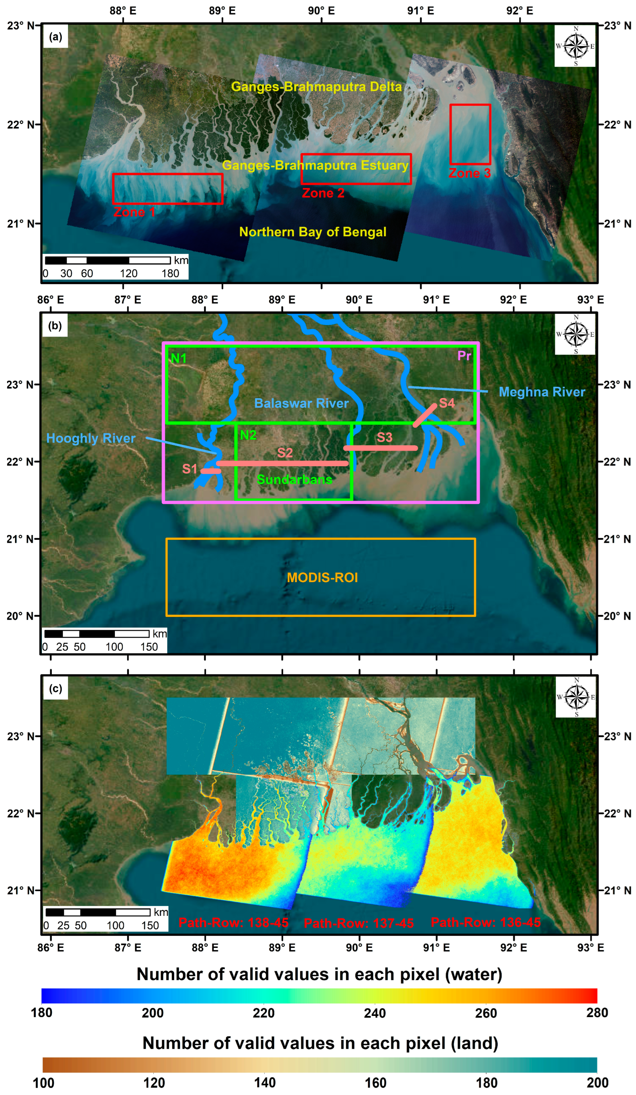
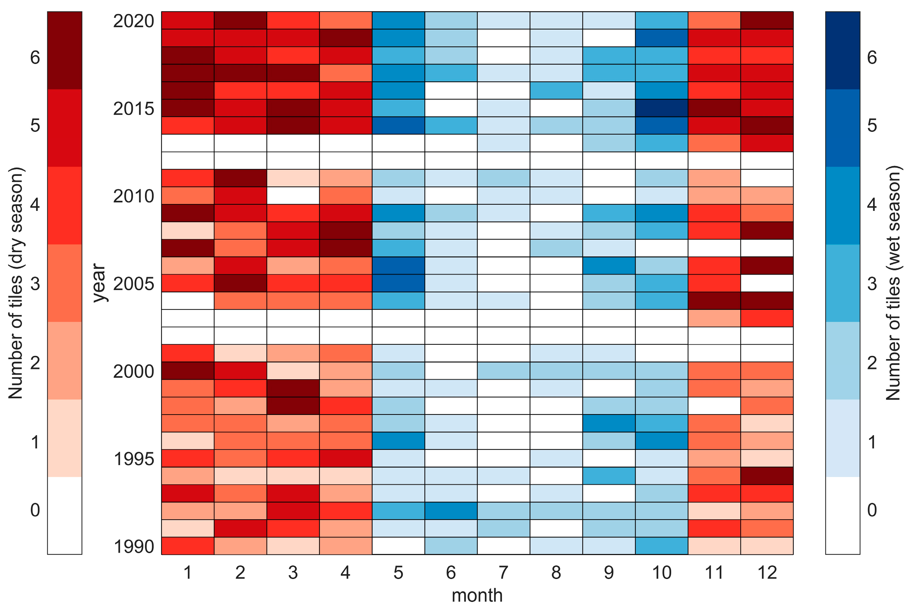

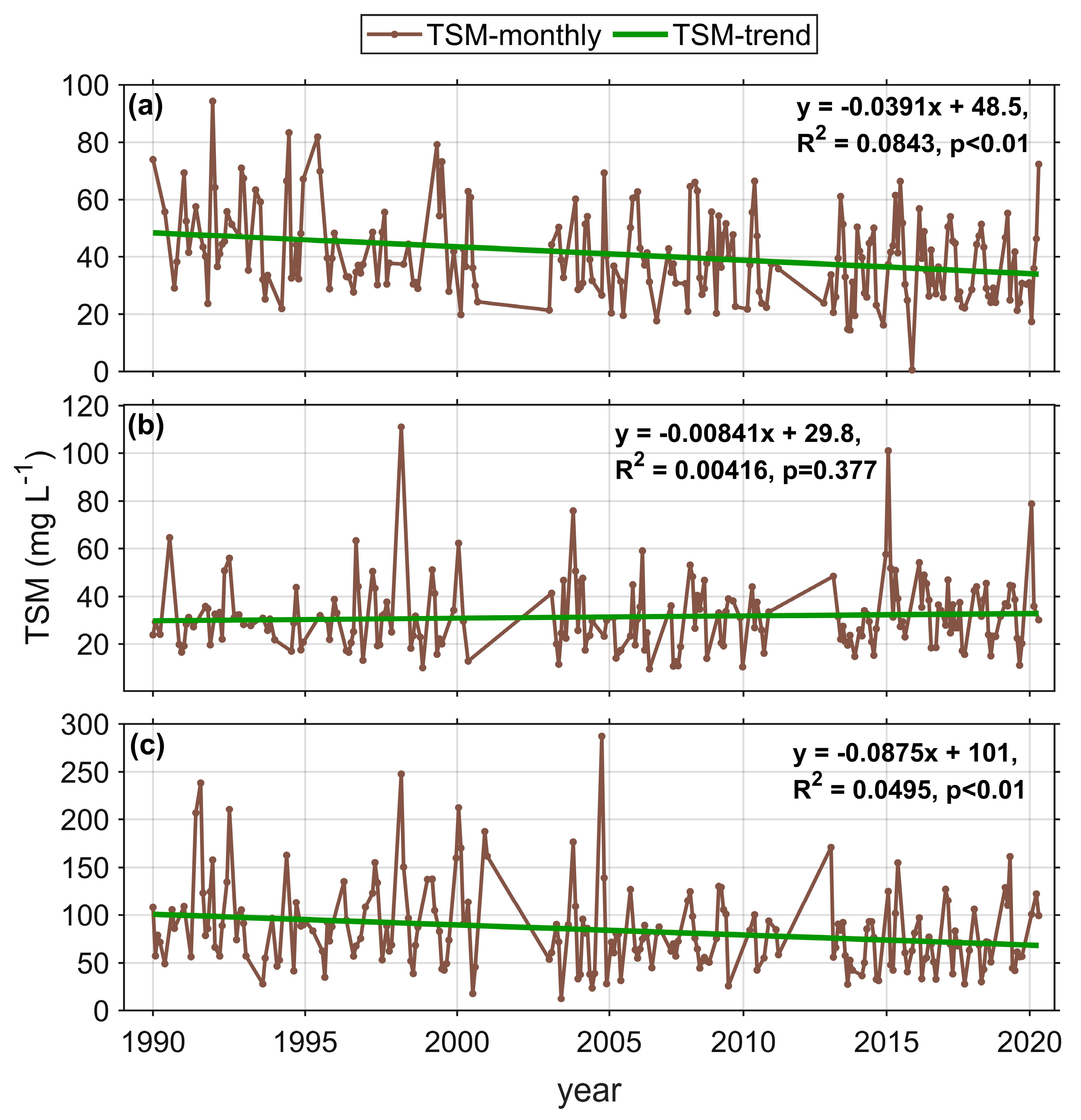
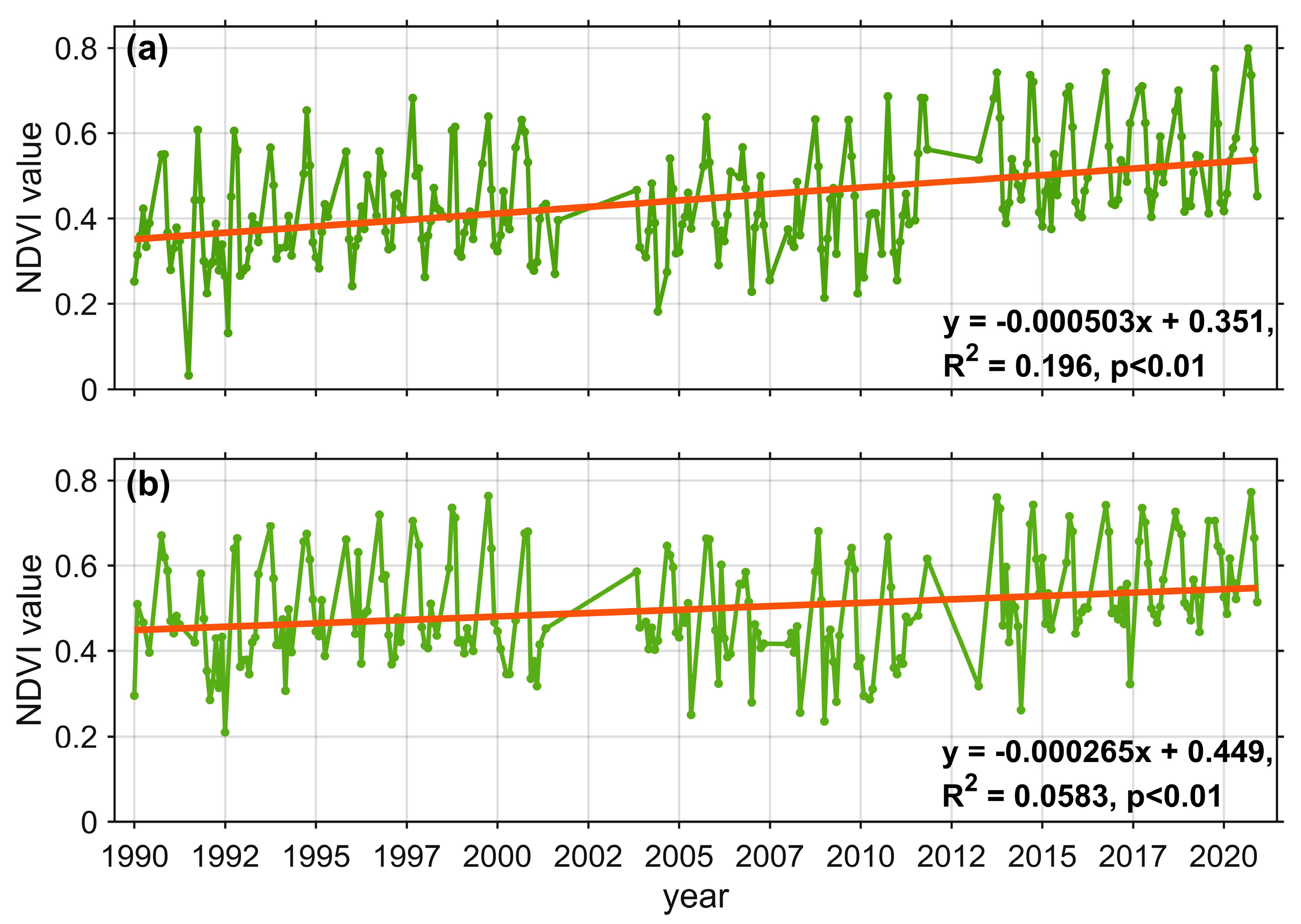
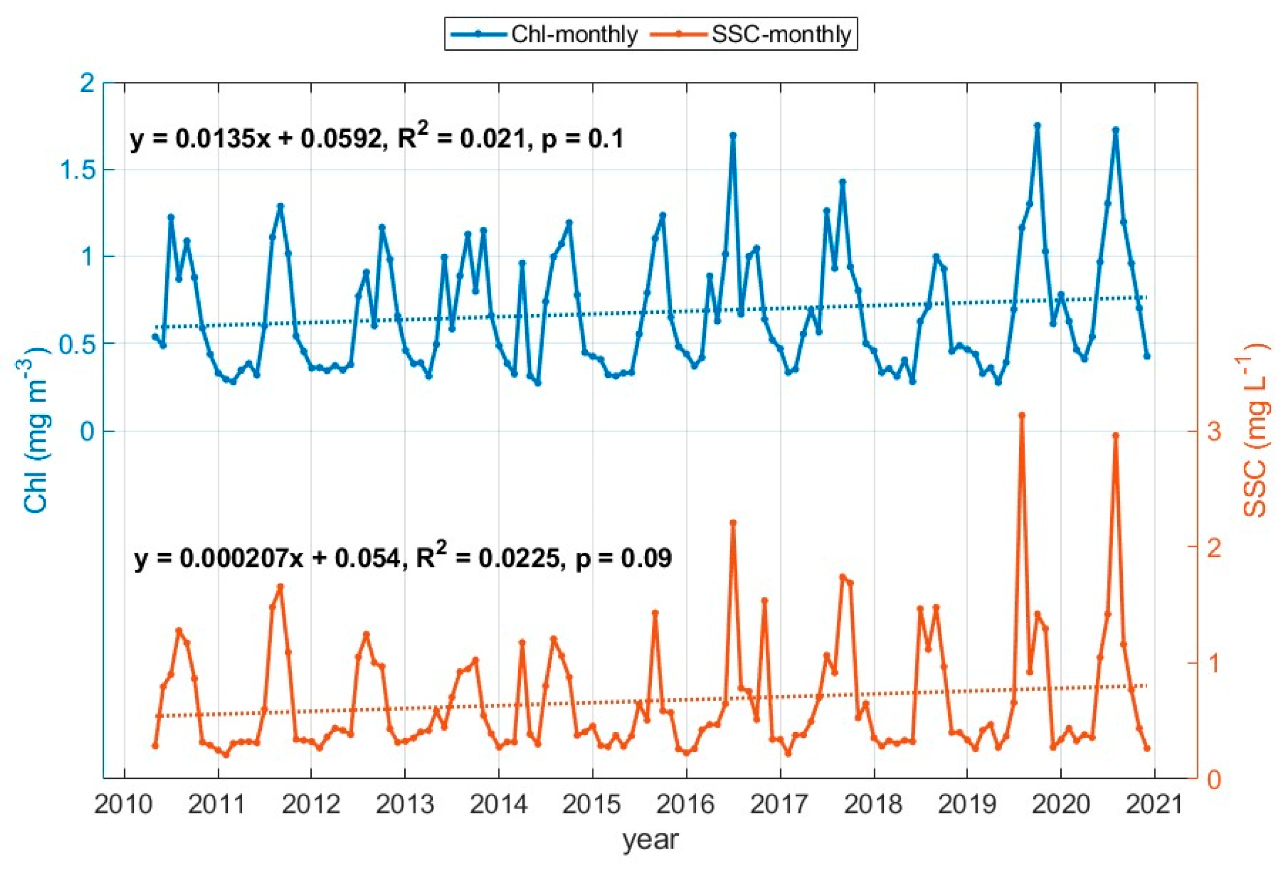

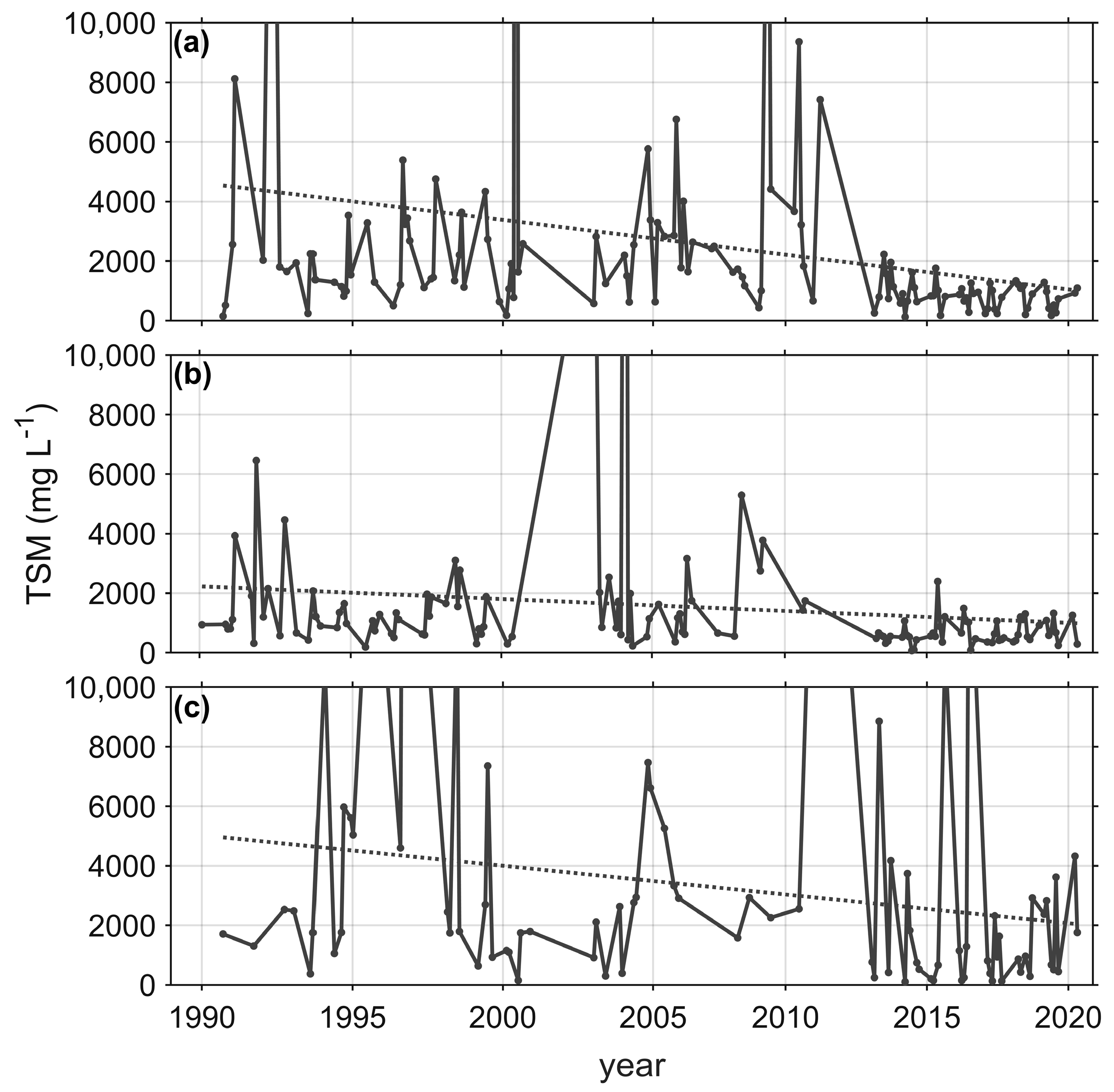
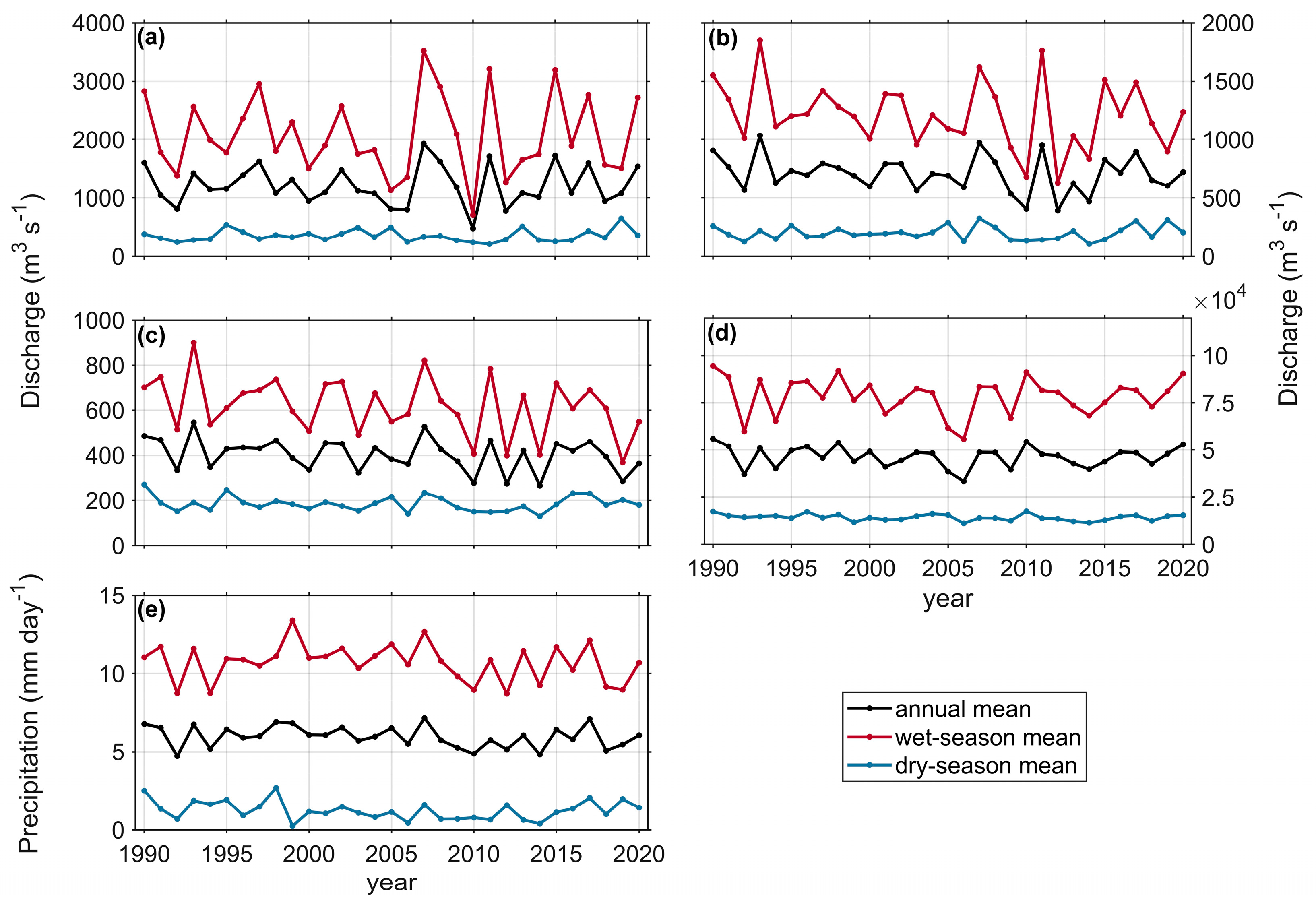
Disclaimer/Publisher’s Note: The statements, opinions and data contained in all publications are solely those of the individual author(s) and contributor(s) and not of MDPI and/or the editor(s). MDPI and/or the editor(s) disclaim responsibility for any injury to people or property resulting from any ideas, methods, instructions or products referred to in the content. |
© 2024 by the authors. Licensee MDPI, Basel, Switzerland. This article is an open access article distributed under the terms and conditions of the Creative Commons Attribution (CC BY) license (https://creativecommons.org/licenses/by/4.0/).