Abstract
In this paper, we complete pioneering research that indicates the very low frequency (VLF) signal amplitude and phase noise reductions, and short-period wave excitations and attenuations as new potential earthquake precursors. We consider changes in the VLF signal broadcast in Italy by the ICV transmitter and recorded in Serbia that start a few tens of minutes before earthquakes. The sampling interval of the analyzed data is 0.1 s. The main objectives of this study are (1) to complete this research in the time and frequency domains during the periods of the four earthquakes analyzed in the previous studies, and (2) to define the parameters of the VLF signal amplitude and phase in both domains that should be further examined in statistical analyses of the aforementioned potential earthquake precursors. In the first part of this study, we analyze the ICV signal amplitude in the frequency domain during the period around three earthquakes that occurred in November 2010 near the considered signal propagation path. Here, we apply the Fourier transform to the relevant recorded data. In the second part, we compare characteristics of the signal amplitude and phase noise reductions in the time domain, and wave excitations and attenuations in the frequency domain. The results of these comparisons indicate the parameters that should be analyzed in subsequent studies to confirm the connection of the considered VLF signal changes with seismic activity before earthquakes, and potentially establish procedures for their detection are: (a) the start and end times of the noise reductions in the time domain and the excited/attenuated waves in the frequency domain, (b) the differences in the corresponding times, and (c) the wave periods of wave excitations of both the signal amplitude and phase.
1. Introduction
The application of electromagnetic signals in ionospheric observations allows obtaining sets of various types of data. Their processing produces results important to both research in several scientific disciplines and research that has practical applications. One of the directions in the analysis of these data refers to the examination of possible ionospheric disturbances that precede earthquakes. Although the first studies on this topic were published in the sixties of the last century [1,2], the most important goal of these studies, the establishment of a sufficiently reliable method for predicting this natural disaster, has not yet been achieved. The most important reasons for that are the complexity of the cause-and-effect relationships between processes in the lithosphere and atmosphere, the existence of numerous processes in the Earth’s layers and outer space that simultaneously affect the area at ionospheric heights and also the lack of observational data with the necessary temporal and spatial resolutions. However, the importance of this goal makes these studies actual in all previous decades [3,4]. Moreover they have been intensified at the global level in recent years [5,6,7].
One of the techniques for monitoring the ionosphere is based on the propagation of very low frequency (VLF) radio signals. These signals propagate in the so-called Earth-ionosphere waveguide from transmitters to receivers that are distributed around the world. The emission of these signals is continuous, and the data can be detected with a time resolution of several ms, which makes it possible to obtain information related to both short-term disturbances (e.g., caused by lightning [8]) and unpredictable phenomena, among which earthquakes are included [9,10,11].
In previous research, the variations in VLF signals before earthquakes indicate a time shift of the characteristic minima of their amplitudes in the periods of sunrise and sunset [4,12,13], and a significant increase or decrease in these values as well as their oscillatory temporal evolution in some periods [14,15,16,17,18]. These changes are generally noted a few days or weeks before strong earthquakes, and, as in the case of seismic process research in other scientific disciplines (see for example [19]), they can be detected in time and frequency domains.
In addition to analyses of the main tendencies of some physical quantities or characteristics of signals used for the corresponding observations, analyses of the noise of relevant parameters can also be used to investigate phenomena such as seismic processes [20,21]. The recent analyses of both VLF signal parameters (amplitude and phase) in the time and frequency domains indicate potentially new effects that occur a few minutes or tens of minutes before an earthquake: (a) the reductions in the amplitude and phase noises (visible in the time domain and defined as the maximum absolute values of the deviations of the recorded amplitude and phase values from the relevant smoothed curves obtained after elimination p percent of their largest and lowest values in the considered time intervals), and (b) the wave excitations and attenuations (visible in frequency domain) [11,22]. In these two studies, the ICV signal emitted in Italy and received in Serbia is analyzed in the periods around the four earthquakes of magnitude greater than 4 that occurred in Serbia near Kraljevo (K1) and in the Tyrrhenian Sea (TS) on 3 November 2010, near Kraljevo (K2) on 4 November 2010, and in the Western Mediterranean Sea (WMS) on 9 November 2010. The obtained results show the following:
- Time domain: the reductions in the amplitude and phase noises are visible before all four earthquakes ([11] and [22], respectively);
- Frequency domain: the excitations and attenuations of waves manifested as increases and decreases in the Fourier amplitude before the earthquake at different wave periods are recorded for
- -
- the amplitude in the case of the K1 earthquake [11], and
- -
- the phase for all four considered cases [22].
These two studies are the first studies that investigate the reductions in the VLF signal amplitude and phase noises, as well as the excitations and attenuations of waves with small periods in their time evolutions before earthquakes. In other words, we can consider them as pilot studies of these potential earthquake precursors. However, these studies do not provide a complete analysis of the VLF signal changes before the observed four earthquakes because the amplitude analysis in the frequency domain is given only for the period around the K1 earthquake. For this reason, we complete this research in the first part of this study giving analyses of the recorded wave extinctions and attenuations in the periods around the remaining three earthquakes.
Although these two studies are based on a small number of earthquakes, the obtained results clearly indicate specific types of changes which, bearing in mind the importance of earthquake prediction, should be statistically examined in future studies. For this reason, in the second part of this study, we define the parameters for determining the described changes in a VLF signal that should be analyzed in investigations of possible earthquake precursors in the following studies. Here, we used the results obtained in the first part of this study, and in [11,22]. In that way, this study concludes the described pilot investigation and provides guidance for appropriate further research.
This paper is organized as follows. The observations, and data processing are described in Section 2. The obtained results are presented in Section 3. In particular, the results related to the analysis of the amplitude in the frequency domain in the periods around the TS, K2, and WMS earthquakes and their comparisons with previous results are given in Section 3.1, while the determination of the signal amplitude and phase parameters that should be analyzed in future statistical studies of the indicated possible earthquake precursors are shown in Section 3.2. Finally, the conclusions of this study and guidance for appropriate further statistical analyses are given in Section 4.
2. Observations and Data Processing
2.1. Observational Setup and Studied Earthquake Events
This paper provides an analysis of the amplitude of the 20.27 kHz VLF signal emitted by the ICV transmitter located in Isola di Tavolari, Sardinia, Italy (40.92°N, 9.73°E). The presented data are recorded at the Institute of Physics Belgrade in Belgrade, Serbia, (44.8°N, 20.4°E) by the Absolute Phase and Amplitude Logger (AbsPAL) VLF receiver with sampling periods of 0.1 s during 3, 4 and 9 November 2010. This receiving setup is developed by the Radio and Space Physics Group of Otago University, New Zealand, and consists of the electric VLF antenna, the GPS antenna, the VLF preamplifier, feed cables, the Service Unit, and the DSP (digital signal processor) card for the computer.
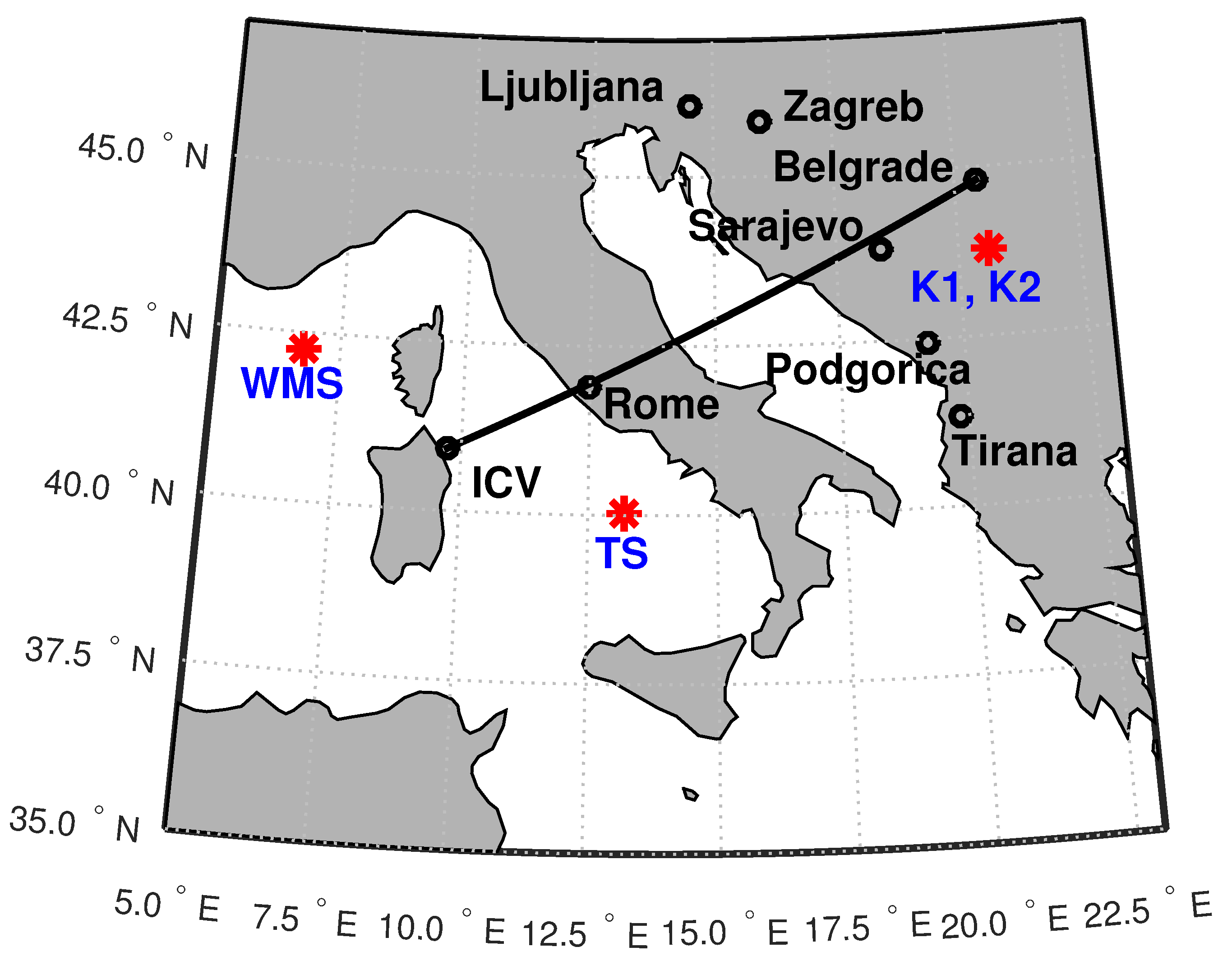
The map with the locations of the used transmitter and receiver and the signal propagation path is given in Figure 1. In this figure, stars represent the epicenters of the considered four earthquakes with magnitude:
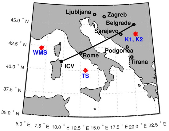
Figure 1.
The VLF signal propagation path from the ICV transmitter to the Belgrade receiver station in Serbia. The red stars represent the epicenters of the considered earthquakes in the Tyrrhenian Sea (TS), Western Mediterranean Sea (WMS), and the two earthquakes near Kraljevo K1 and K2 (the same star shows them).
- Mw 5.4 that occurred near Kraljevo (K1; 43.74°N, 20.69°E) on 3 November 2010;
- mb 5.1 that occurred in the Tyrrhenian Sea (TS; 40.03°N, 13.2°E) on 3 November 2010;
- ML 4.4 that occurred near Kraljevo (K2; 43.78°N, 20.62°E) on 4 November 2010 (since this location is very close to the location of the K1 earthquake epicentre, the same star refers to both these earthquakes);
- ML 4.3 that occurred in the Western Mediterranean Sea (WMS; 42.25°N, 6.77°E) on 9 November 2010.
The above data are provided on the website of the Euro-Mediterranean Seismological Centre [23]. The symbols Mw, mb and ML denote the moment magnitude [24], body-wave magnitude [25] and Richter [26] scales, respectively. The relations between their values are complex [27], and some of them are shown in statistical studies (see, for example, [28,29]).
The shortest distances of the epicenters of the mentioned earthquakes from the observed VLF signal propagation path are 126 km, 219 km, 114 km and 287 km, respectively.
2.2. Data of the ICV Signal Amplitude Analyzed in Detail in This Study
The time evolutions of the ICV signal amplitude, A, recorded by the AbsPAL receiver during the periods around the TS, K2, and WMS earthquakes are shown in Figure 2. The vertical lines indicate the times of all earthquakes that occurred close to the observed signal path (data on these earthquakes and the distances of their epicenters from the path of the observed signal are given in [22,23]). The times of occurrences of the considered three events are indicated by the vertical red dash lines.
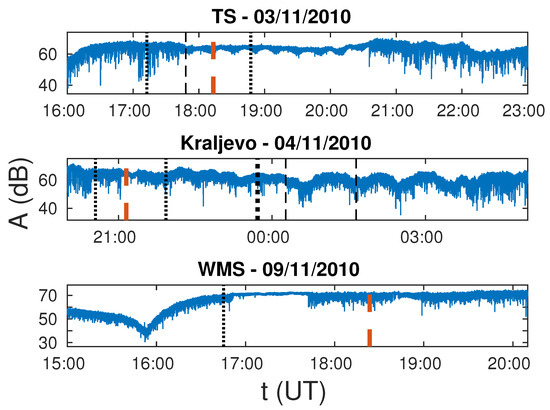
Figure 2.
The ICV signal amplitude for time periods around the TS (upper panel), K2 (middle panel) and WMS (bottom panel) earthquakes. The vertical dashed red lines indicate these earthquakes, while the vertical black lines indicate additional earthquakes with magnitudes below 2.5 (thin dotted lines), between 2.5 and 3 (thin dashed lines), and between 3 and 4 (tick dotted line).
In Figure 2, it can be seen that the amplitude noise reduction is most pronounced before the strongest earthquakes in all three observed time intervals. Additional two, and four earthquakes during 3 and 4 November, respectively, occurred during the period of visible amplitude noise reduction in relation to its values at the beginnings and ends of the respective time intervals. In the third time interval, the amplitude noise reduction is visible only before the strongest earthquake, but it is interrupted during a shorter period (including the time of the earthquake). This interrupted part may indicate the existence of a short-term additional source of the noise, or that the corresponding connection should be established only with the second noise amplitude reduction. The delay of minutes of this amplitude noise reduction in relation to the time of the earthquake can potentially be explained by the greater distance of the epicenter from the signal path, and/or the fact that it is moved from that route in the sense that the shortest considered distance is the one to the transmitter. The most pronounced amplitude noise reduction is visible in the case of the first observed earthquake with the strongest magnitude.
2.3. Data Processing
As stated in the Introduction, analyses of VLF and LF signals show changes in both their parameters (amplitude and phase) before the occurrence of an earthquake. In this paper, analyses of the characteristics of changes in both these parameters of the ICV signal are provided in the time and frequency domains. These procedures are described in detail in the first study of the appropriate amplitude noise reduction [11]. Here, we will only list their basic characteristics.
2.3.1. Data Analyses in the Time Domain
To determine changes in the time domain, the time evolutions of the amplitude and the phase are processed. Although the processing of these data for determining the amplitude noise using the method given in [11] consists of two phases (1. determining the deviation of the recorded values from the relevant smoothed curve dA, and 2. determining the defined in [30] as the maximum absolute values of dA after removing p percent of their highest values due to the elimination of potential short-term influences of other phenomena), only the first part is applied in this study. The reason is the better precision in the estimation of the time of the observed changes because is calculated for certain time intervals, and not for every time t. This is especially important in the cases where the intervals in which the amplitude and phase noise decrease are only a few minutes. Because the observed changes are not instantaneous, their times are set at 30 s. In other words, the error of determining the start and end times of the amplitude and phase noise reductions is 30 s. Bearing in mind that the critical values of the parameters characterizing the noise level reduction must be determined in analyses with a statistically significant sample, in this study the reduction in the amplitude and phase noises are determined visually.
2.3.2. Data Analyses in the Frequency Domain
As we said in the Introduction, in the first part of this study, we provide a detailed analysis of the ICV signal amplitude in the frequency domain for the time periods around the TS, K2, and WMS earthquakes. As in the relevant analyses given in [11,22], we apply the Fast Fourier Transform (FFT) to the data shown in Figure 2 (recorded in the time domain) in the windows time intervals (WTIs) of 20 min, 1 h, and 3 h. In all three cases, the steps between two neighboring WTIs are 10 min. The obtained results represent the Fourier amplitudes that depend on the wave period , where f is frequency, while the increase and decrease in its values in time indicate the excitation or attenuation of the wave at the observed T, respectively. The analysis of these changes in the frequency domain is the focus of the first part of this study, while the obtained results are included in the second part, where the parameters relevant for statistical analyses of the amplitude and phase noise reductions and the obtained changes in for all four events are compared to define parameters which should be analyzed as a possible earthquake precursor in the forthcoming statistical studies.
To obtain the considered times with the lowest error we determine them from the results for WTI = 20 min. In this case, errors in the determination of the time t, wave period T, and Fourier amplitude are:
- The error in the time determinations is the step between two WTIs, e.g., 10 min.
- The error in the determination of T is not the same because these values are not equidistant (in FFT the values of frequency f are equidistant), and depends on its values. It can be determined in two ways:
- -
- In the case of high frequencies, e.g., low wave periods (here, we consider the maximum value for this case of 1 min) for which the differences of adjacent values are small, an approximate determination of the error is made from the relationship between the wave period and frequency (), and the error of frequency : where (for WTI of 20 min, 1 h and 3 h, the values of are 8.3333 × 10 Hz, 2.7778 × 10 Hz, and 9.2593 × 10 Hz, respectively).
- -
- In the case of lower frequencies, i.e., the wave periods longer than 1 min, the error is determined by the absolute difference of a certain value of T and the first more discrete value of this parameter.
- For the same reason as in the case of determining the reduction of the amplitude and phase noise, the increasing and decreasing of is determined visually.
2.4. Comparisons of the Parameters Relevant for the Statistical Analyses Related to the Considered Possible Earthquake Precursors
As stated in the Introduction, the determination of the parameters that are relevant for the statistical analyses of the amplitude and phase noise reductions, and the excitation and attenuation of short-period waves is based on the comparisons of the results presented in the first part of this study as well as in [11,22]. An overview of the data sources for the ICV signal amplitude and phase in the time and frequency domains in the periods around the considered K1, TS, K2, and WMS earthquakes is given in Table 1.

Table 1.
Data sources for the ICV signal amplitude and phase for the analyses in the time and frequency domains in the periods around the considered K1, TS, K2, and WMS earthquake occurrences.
Based on the previous two indicated studies, these changes are manifested as:
- The reductions in the VLF signal amplitude and phase noises in the time domain;
- The excitations of waves at discrete low values of wave periods (below 1.5 s) and the attenuations of waves at other wavelengths that may have upper limit values after which changes are not observed. These effects are visible in the frequency domain.
In order to determine the parameters that should be further analyzed in statistical studies (they are the main results of this overall pilot research), we compare the times of the beginnings and endings of the mentioned changes in both domains, and the characteristic values of the wave periods in which changes are observed in the frequency domain.
3. Results and Discussion
As we stated in the previous text, the results of this research and their analyses are presented in two parts. In the first part (Section 3.1), we present the investigation of the signal amplitude in the frequency domain during the periods around the earthquakes that occurred in the Tyrrhenian Sea (TS earthquake) on 3 November 2010, near Kraljevo (K2 earthquake) on 4 November 2010, and in the Western Mediterranean Sea (WMS earthquake) on 9 November 2010. Comparisons of the results given in [11,22], and Section 3.1 and related to the ICV signal amplitude and phase in the time and frequency domains for all four considered earthquakes are presented in Section 3.2.
3.1. Analysis of the Signal Amplitude in the Frequency Domain
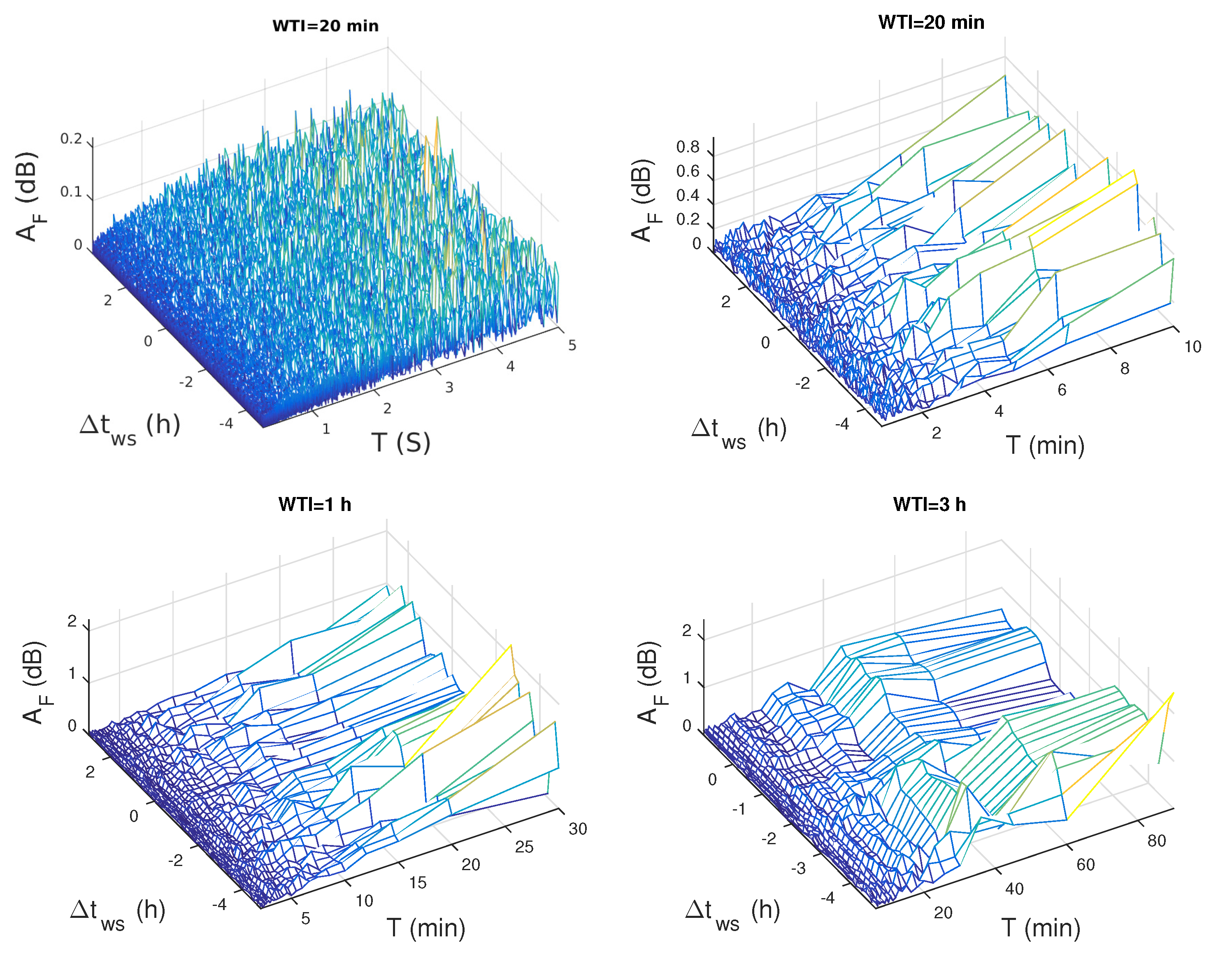
The dependences obtained by applying the procedure described in Section 2 to the data recorded during a quiet period, and the periods around the TS, K2, and WMS earthquakes (presented in Figure 2) are shown in Figure 3, Figure 4, Figure 5 and Figure 6, respectively. In these figures, we consider the window time intervals (WTIs) of 20 min, 1 h and 3 h. The x-axes show the times of the beginnings of those intervals in relation to the time when the main analyzed earthquake in the considered day is registered (). In the case of the shortest WTI of 20 min, the obtained dependencies are divided into two graphs in order to separate the dependencies for s and s due to the large difference in values.
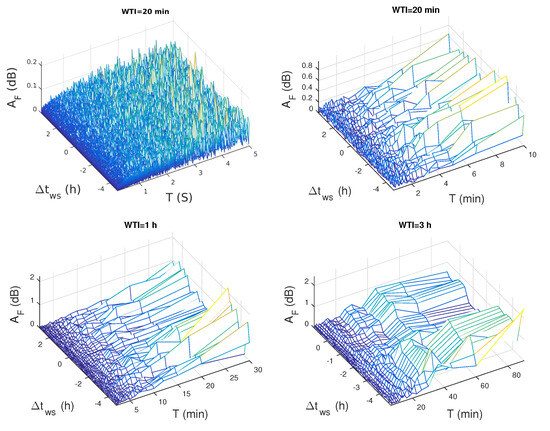
Figure 3.
The Fourier amplitude of waves with the period T obtained by applying the FFT to the ICV signal amplitude recorded in the quiet period from 19:00 UT on 3 November 2009 to 4:00 UT on 4 November 2009, with the window time intervals (WTI) of 20 min (upper panels), 1 h (bottom left panel), and 3 h (bottom right panel) which begin with a shift with respect to the midnight.

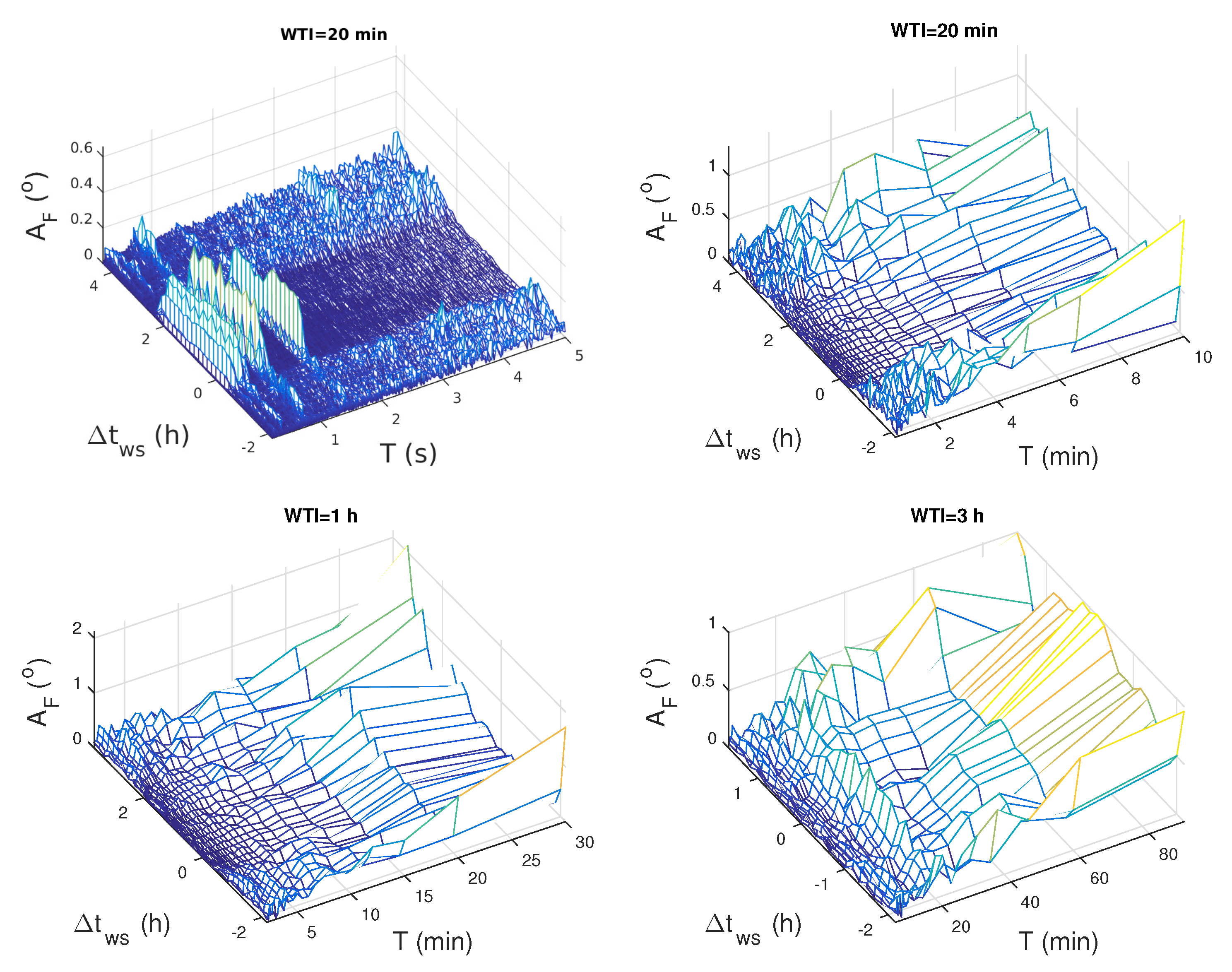
Figure 4.
The Fourier amplitude of waves with the period T obtained by applying the FFT to the ICV signal amplitude recorded in time around the TS earthquake occurred on 3 November 2010, with the window time intervals (WTI) of 20 min (upper panels), 1 h (bottom left panel), and 3 h (bottom right panel) which begin with a shift with respect to the TS earthquake time.
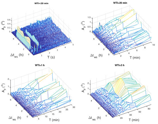
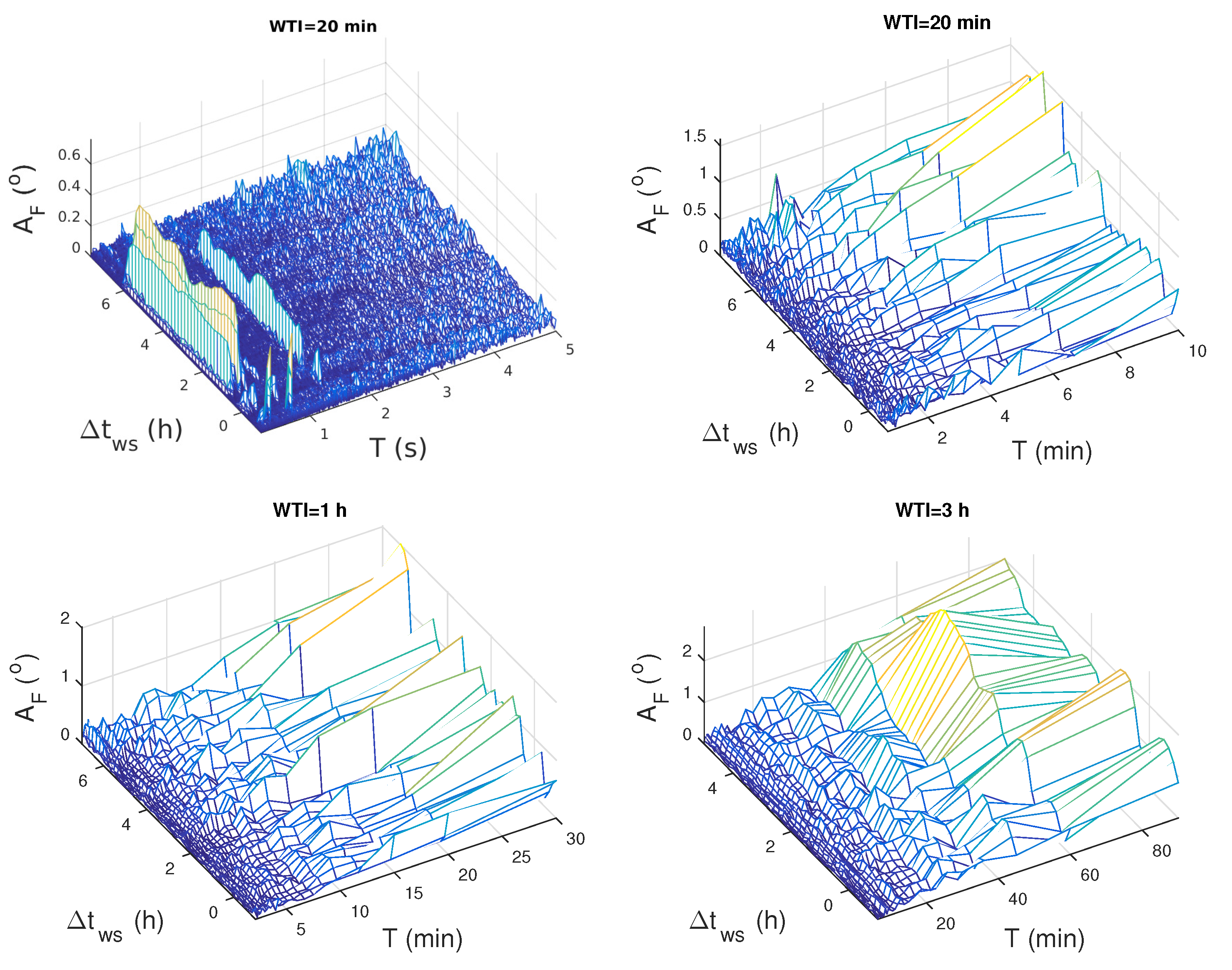
Figure 5.
The Fourier amplitude of waves with the period T obtained by applying the FFT to the ICV signal amplitude recorded in time around the K2 earthquake occurred on 4 November 2010, with the window time intervals (WTI) of 20 min (upper panels), 1 h (bottom left panel), and 3 h (bottom right panel) which begin with a shift with respect to the K2 earthquake time.
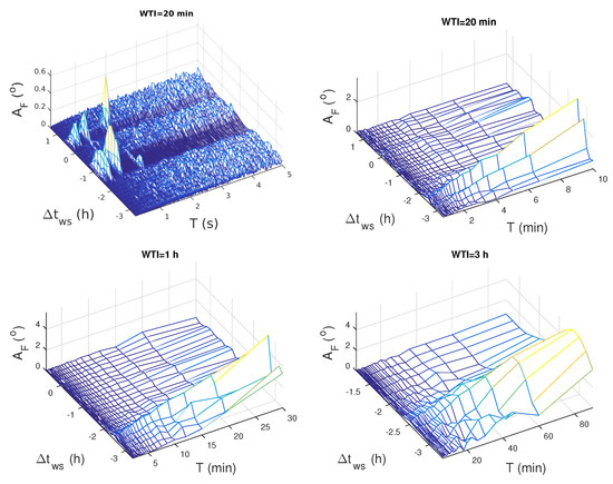
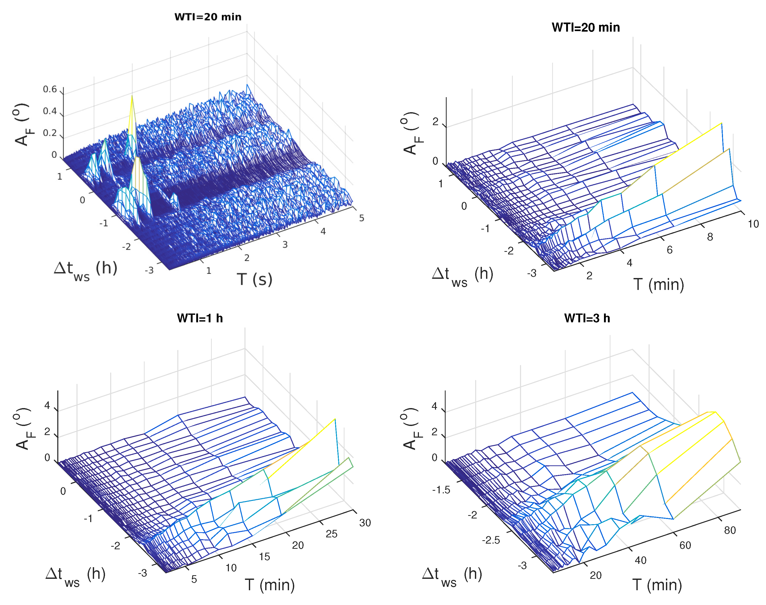
Figure 6.
The Fourier amplitude of waves with the period T obtained by applying the FFT to the ICV signal amplitude recorded in time around the WMS earthquake occurred on 9 November 2010, with window time intervals (WTI) of 20 min (upper panels), 1 h (bottom left panel), and 3 h (bottom right panel) which begin with a shift with respect to the WMS earthquake time.
3.1.1. Analysis of the ICV Signal Amplitude in a Quiet Period
To rule out the influence of periodic variations on signal propagation characteristics, we apply the FFT to the time evolution of the ICV signal amplitude from 19:00 UT on 3 November 2009, to 4:00 UT on 4 November 2009, when there were no significant impacts of sudden events (including earthquakes) on the considered VLF signal [11]. The obtained results presented in Figure 3 show the following:
- Increases and decreases in in time are not recorded in the upper panels showing the results for WTI = 20 min. In other words, excitations and attenuations of waves with a wave period below 10 min are not visible.
- has higher values during the periods of sunset and sunrise, which is a consequence of intense variations in the signal amplitude time evolution, which include pronounced minima (see, for example, [31,32]). Here, we emphasize that the variations in last for a long time because specific data provide integral information for the relevant time interval WTI to which the FFT is applied.
Bearing in mind these conclusions in the case of a quiet period, we will exclude the mentioned variations on larger wave periods for WTI of 1 h and 3 h from the following analyses related to the time periods around the considered three earthquakes.
3.1.2. Analysis of the ICV Signal Amplitude in the Period around the TS Earthquake
The TS earthquake occurred in the Tyrrhenian Sea at 18:13:10 UT on 3 November 2010. In the considered time period around this earthquake (16:00 UT–23:00 UT on 3 November 2010), the three smaller ones are recorded near the propagation path of the considered ICV signal (the two before and the one after the TS earthquake). Their characteristics are given in Table 2.
Table 2.
Characteristics of the earthquakes that occurred in the considered period around the TS earthquake: the occurrence time t, the latitude (LAT) and longitude (LON) of the epicenter positions, the magnitude, and the locations. The shown data are given in [23] and used in [22].
The visualization of wave excitations and attenuations in this time period is given in Figure 4 which shows the time evolutions of at discrete values of T. The following characteristics of the most pronounced changes visible in this figure are:
- As in the studies presented in [11,22], the wave excitations are visible at small discrete values of the wave periods below 1.5 s. They can be seen in the upper left panel for WTI = 20 min (for smaller values of T) in the time interval starting (40 ± 10) min before the TS earthquake and ending (130 ± 10) min after it. The specific values of the periods of the excited waves are (0.2333 ± 0.0001) s, (0.2800 ± 0.0001) s, (0.3500 ± 0.0002) s, (0.4667 ± 0.0002) s, (0.7001 ± 0.0005) s, and (1.400 ± 0.002) s. The stated errors are determined based on the explanation given in Section 2. A clearer representation of the jumps representing the indicated wave excitations is shown in Figure 7 where the dependencies (in moments when wave excitations are visible) are given for all four considered cases.
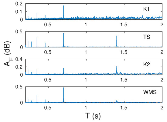 Figure 7. The Fourier amplitude obtained by applying the FTT to the ICV signal amplitude during excitations of waves with periods less than 2 s in the time intervals around the K1, TS, K2, and WMS earthquake occurrences (panels are shown, respectively, from top to bottom) with period T.
 - The wave attenuations, manifested as decreases in , are recorded for all values of T from its minimum value to 15 min except for those at which the indicated wave excitations are visible. They occur in similar time intervals as the mentioned excitations (determined on the panels for WTI = 20 for the best accuracy). The value of 15 min is determined in the graph for WTI = 1 h (lower left panel in Figure 4) because of better precision than in the case for WTI = 3 h (lower right panel). Here, we emphasize that this determination is not relevant for WTI = 20 min since the maximum value of T in that case is 10 min (half of WTI).
The time period in which the mentioned wave excitations occur includes the times of the TS earthquake and the second and third earthquakes given in Table 2. In addition, the weaker increases in are visible in the time interval when the first earthquake listed in the mentioned table occurred.
3.1.3. Analysis of the ICV Signal Amplitude in the Period around the K2 Earthquake
The K2 earthquake occurred near Kaljevo in Serbia at 21:09:05 UT on 4 November 2010. As can be seen in Table 3, the five smaller ones (the one before, and the four after the K2 earthquake) are recorded near the propagation path of the considered VLF signal during the considered time period (20:00 UT on 4 November–05:10 UT on 5 November 2010).
Table 3.
Characteristics of the earthquakes that occurred in the considered period around the K2 earthquake: the occurrence time t, the latitude (LAT) and longitude (LON) of the epicenter positions, the magnitude, and the locations. The shown data are given in [23] and used in [22].
The obtained values of for the considered three WTIs are shown in Figure 5. As in the previous case, the excitations and attenuations of the waves, which can be considered as potential earthquake precursors, are visible in multiple time intervals: the first can be associated with the earliest earthquake, the second includes the time of the K2 earthquake and the longest third during which the remaining four earthquakes were recorded. This is very important to note because of two facts:
- By the analyses of the signal characteristics in the periods of other earthquakes, the lasting of the wave excitation/attenuation period can be related to the number of earthquakes that occur within a relatively short time period.
- The magnitudes of the additional earthquakes are below 3.5 because that indicates that the dependence of the earthquake intensity and the excited/attenuated waves characteristics are not simple and that their examinations require the analyses of statistically significant samples with the inclusion of additional parameters that characterize the considered earthquakes, positions of their epicenters relative to the considered signal propagation path, signal, and states of the atmosphere.
The characteristics of the excitations and attenuations of the waves that start before the K2 earthquake are:
- The wave excitations are visible in the time interval starting (20 ± 10) min before the K2 earthquake and ending (10 ± 10) min after it at the wave periods of (0.2333 ± 0.0001) s, (0.2000 ± 0.0001) s, (0.2800 ± 0.0001) s, (0.3500 ± 0.0002) s, (0.4667 ± 0.0002) s, (0.7001 ± 0.0005) s, and (1.400 ± 0.002) s. As in the first case, is determined from the upper left panel of the corresponding figure (WTI = 20 min), and the stated errors are determined based on the explanation given in Section 2. Also, a clearer representation of the jumps representing the indicated wave excitations is shown in Figure 7.
- As in the first case, the wave attenuations, manifested as decreases in , are visible in similar time intervals as the mentioned excitations for all values of T from its minimum value to 6.667 min except for those at which the indicated wave excitations are visible (see the both upper panels for WTI = 20 min, and the bottom left panel for WTI = 1 h).
3.1.4. Analysis of the ICV Signal Amplitude in the Period around the WMS Earthquake
The WMS earthquake occurred in the Western Mediterranean Sea at 18:23:36 UT on 9 November 2010. In this case, one additional earthquake occurred before it in the considered time period (15:00 UT–20:10 UT on 9 November 2010). Their corresponding characteristics are given in Table 4, while the obtained dependencies are presented in Figure 6.
Table 4.
Characteristics of the earthquakes that occurred in the considered period around the WMS earthquake: the occurrence time t, the latitude (LAT) and longitude (LON) of the epicenter positions, the magnitude, and the locations. The shown data are given in [23] and used in [22].
In this case, the two time periods when the already explained wave excitations and attenuations exist are visible. The first of them occurs before the WMS earthquake but also ends before it. The other typical changes occur soon after. A possible explanation for this interruption could be some source of noise in that period. In addition, the position of this earthquake with respect to the signal path differs from those in the previous two cases: (a) the distance of the location of its epicenter from the signal path is the greatest, (b) the closest part of the signal path to it is the ICV transmitter. Also, it should be emphasized that the WMS earthquake is preceded by a weak earthquake. However, although noise amplitude reductions are also recorded in cases of earthquakes of magnitude below 3 [11], in this case, the reduction is detected after that earthquake, which is why it cannot be considered as its precursor. Of course, this does not exclude the possibility of a subsequent change in the characteristics of the VLF signal, but connecting them requires better statistics. In the following analysis, we assume that both mentioned periods are associated with the WMS earthquake.
The characteristics of the explained excitations and attenuations (determined in the same way as in the previous two cases) are:
- The wave excitations are visible in the time interval starting (100 ± 10) min before the WMS earthquake and ending (30 ± 10) min after it at the wave periods of (0.2333 ± 0.0001) s, (0.2800 ± 0.0001) s, (0.3500 ± 0.0002) s, (0.4667 ± 0.0002) s, (0.7001 ± 0.0005) s, and (1.400 ± 0.002) s (see Figure 7).
- As in the first case, the wave attenuations manifested as decreases in , are visible in similar time intervals as the mentioned excitations for all values of T from its minimum value to 5.455 min except for those at which the indicated wave excitations are visible (see both upper panels for WTI = 20 min, and the bottom left panel for WTI = 1 h).
3.1.5. Comparisons of the Obtained Results
The common characteristics of the observed changes in all three cases are:
- The beginnings of changes in are recorded before the time of the earthquake;
- Wave excitations are most pronounced for discrete values of period T below 1.5 s;
- The best representation of wave excitations is obtained for minimum time intervals of 20 min;
- Wave attenuations during those time intervals are pronounced for other periods below several minutes.
The obtained conclusions are in accordance with those obtained in the analysis of the ICV signal amplitude in the period around the earthquake near Kraljevo of magnitude 5.4 that occurred on 3 November 2010 [11]. A comparison with the results of the Fourier transformation of the ICV signal phase in the periods around these four earthquakes presented in [22] show similar time periods when excitations/attenuations are visible, similar values of T for which wave excitations are recorded, but also significantly larger domains of T for which the attenuation in waves of phase is visible.
3.2. Defining of VLF Signal Amplitude and Phase Parameters in the Time and Frequency Domains as Potential Earthquake Precursors
Based on the results presented in Section 3.1, and the studies given in [11,22], the changes in the VLF signal amplitude and phase can be classified
- In the time domain according to:
- -
- Characteristics of the amplitude/phase noise reduction,
- In the frequency domain according to:
- -
- Characteristics of excited waves before an earthquake at discrete values of the wave periods lower than 1.5 s,
- -
- Characteristics of attenuated waves on other wave periods with or without visible limitations in the upper limit of the observed domain.
To determine directions in further research of possible earthquake precursors manifested in the reduction in the VLF signal amplitude and phase noises, and the wave excitations and attenuations at small wave periods, we provide the following comparisons and we analyse the effects of other earthquakes on the duration of the mentioned changes.
- In the time domain:
- -
- The start time of the amplitude/phase noise reduction in relation to the time of the considered earthquake,
- -
- The end time of the amplitude/phase noise reduction in relation to the time of the considered earthquake;
- In the frequent domain:
- -
- The start time of the wave excitation/attenuation in relation to the time of the considered earthquake,
- -
- The end time of the wave excitation/attenuation in relation to the time of the considered earthquake,
- -
- Discrete values of of the excited waves,
- -
- The upper limit of the wave period domain within the wave attenuation is visible;
Here, we emphasize once again that this analysis is a pilot study and that its goal is to determine the parameters that, based on the observed sample, indicate possible changes that are potential precursors of earthquakes, their relationship and comparison of the quality and clarity of their detection. In addition to these parameters, future statistical studies should also include additional ones whose analysis requires a larger number of events. Here, we primarily mean the influence of earthquake characteristics (magnitude, depth) and the relative position of the earthquake epicentre and the path of the observed signal, the state of the atmosphere (primarily daytime, nighttime and solar terminator periods) on the characteristics of signal disturbances.
3.2.1. Intervals of Changes in the Time and Frequency Domains
Comparisons of the considered start and end times of changes in the time ( and , respectively) and frequency ( and , respectively) domains for the amplitude and phase are shown in Table 5, where it is assumed that the time intervals of the wave excitation and attenuation are the same for an earthquake (based on the obtained dependences ). To obtain the most accurate results, the displayed times are determined from the analysis of the graphs obtained for the smallest considered WTI of 20 min. As we stated in Section 2.3, the errors of determining the analyzed times in the time and frequency domains are 30 s and 10 min, respectively.
Table 5.
The start and end times (with respect to the times of the K1, TS, K2, and WMS earthquakes) of the noise reductions (NR) in the time (t) domain ( and , respectively), and excitations/attenuations in the frequency (f) domain ( and , respectively) of the ICV signal amplitude (A) and phase (P). The errors in determining the analyzed times in the time and frequency domains are 30 s and 10 min, respectively.
The following can be concluded from this table:
- The times and are the same (in three cases) and similar (in the last case) in the time evolutions of the amplitude and phase of the ICV signal, while the time intervals in which the increases in the Fourier amplitude are observed are the same for both signal parameters. Discrepancies in and for the amplitude and phase of 20 min and 2 min, respectively, are recorded in the case of an earthquake that differs from the others in the position of its epicenter in relation to the signal path (the distance is the greatest and it is located to the west of the transmitter), and in the type of the noise amplitude reduction which, according to the study given in [33], indicates the displacement of the amplitude values after the reduction of its noise (it is a reduction in Type II in contrast to other cases where they are reductions in Type I). For this reason, the characteristics that should be the subject of analysis in statistical studies are the relationships between the times and for the signal amplitude and phase, as well as the connection of the discrepancy of these times with the reduction type.
- The times and are the same for the amplitude and phase for all cases.
- The times and , and and are not the same for different events. Although they depend on the occurrence of other earthquakes, the investigation of these parameters depending on the magnitude and depth of the earthquake, and the position of its epicentre in relation to the observed VLF signal propagation path is of essential importance for the analyses of the considered changes as possible precursors of earthquakes. Of course, a sample of a significantly larger number of events that can be observed independently is necessary for that and, as stated earlier, this issue will be the subject of future research.
- The start and end times of disturbances are not the same in the time and frequency domains. Here, it should be kept in mind that the resolution in the second case is worse due to the shift in the time intervals on which the Fourier transform is applied in steps of 10 min, and due to the fact that the results of transformation refer to the entire observed time intervals . Although the comparison of the mentioned times is not relevant due to the given reasons, it is noticeable that the obtained differences are different in different cases. This variation indicates the need for more detailed statistical analysis to determine the existence or non-existence of their dependence on the characteristics of earthquakes and signals.
3.2.2. Characteristics of the Wave Excitations and Attenuation Periods
In addition to the duration of observed disturbance time intervals, two more parameters relevant for the frequency domain can be analyzed as precursors of earthquakes: the periods of wave excitation , and the maximum period at which wave attenuation is noticeable in the period around the considered earthquake occurrence.
The values of are the wave periods for which the is increased in time intervals starting before the moment when the observed earthquake occurred. These increases are visible in the 3D graphics in Figure 4,Figure 5 and Figure 6 in this study, and in the relevant figures shown in [11,22]. In order to more clearly show the values of T at which the peaks in are observed, we give the dependences of for the signal amplitude and phase (at the moments when wave excitations are present) in Figure 7 and Figure 8, respectively.
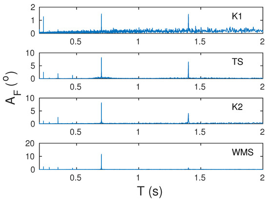
Figure 8.
The Fourier amplitude obtained by applying the FTT to the ICV signal phase during excitations of waves with periods less than 2 s in the time intervals around the K1, TS, K2, and WMS earthquake occurrences (panels are shown, respectively, from top to bottom) with period T.
These values are given in Table 6. In cases where excitations are present for several close periods, the values with the highest are taken.
Table 6.
The wave periods of wave exciatations obtained for the ICV signal amplitude A and phase P for the K1, TS, K2, and WMS earthquakes.
Comparisons of T obtained by Fourier transformation of the A and P time evolutions show the following:
- The periods of the excited waves recorded in the analysis of both the signal amplitude and phase for all four earthquakes are (0.2333 ± 0.0001) s, (0.2800 ± 0.0001) s, (0.3500 ± 0.0002) s, (0.4667 ± 0.0002) s, and (0.7001 ± 0.0005) s. Waves with the period of (1.400 ± 0.002) s are excited in all cases except in the case of the amplitude during the period around the K1 earthquake. (Here, we observe all excitations in contrast to the study given in [22] where only the most significant ones are listed.)
- Wave excitations with (0.2000 ± 0.0001) s are recorded only in the phase analysis for the K1 earthquake, and in the amplitude analysis for the K2 earthquake.
The differences in the obtained characteristics of the Fourier amplitudes obtained from the A and P time evolutions are most noticeable in . In the case of amplitude, these values are significantly smaller and there are no clearly noticeable transitions in the T domains between parts where attenuations are clearly visible, and where they are not significant or do not exist (because of that the relevant values given in Table 7 are estimated). In contrast, reductions in obtained by applying the FFT to are clearly visible for all observed values of T for the K1, TS, and WMS earthquakes. Bearing in mind that the maximum value of WTI is 3 h, the maximum of T shown on the presented graphs is 90 min. For this reason, for these three earthquakes, we can only state that is at least 90 min, but that it most likely reaches higher values. In the case of the K2 earthquake no attenuation is visible for 90 min, which is a consequence of the short time interval within which noise reduction is visible. However, in this case, clear attenuations are also visible for periods of 90 min after this earthquake, when three weaker earthquakes are recorded at locations close to the K2 earthquake epicenter.
Table 7.
The maximum wave periods at which wave attenuation obtained from the amplitude () and phase () time evolutions are noticeable in the period around the considered K1, TS, K2, and WMS earthquake occurrences.
4. Conclusions
In this paper, we complete the first investigation that indicates (a) the reductions in the VLF signal amplitude and phase noises, (b) the excitations of waves in the signal amplitude and phase time evolutions at discrete wave periods below 1.5 s, and (c) the attenuations of waves in the signal amplitude and phase time evolutions at small wave periods as new potential earthquake precursors. This investigation is based on processing the VLF signal amplitude and phase in the time periods around the four earthquakes with magnitudes greater than 4 when the observed signal is not already affected by intensive seismic activities connected with previous strong earthquakes.
In the previous two studies, changes are visible as the noise reduction in both the amplitude and phase in the time domain (analyses are given for all four cases), and as the wave excitations and attenuations in the frequency domain (amplitude analyses are given for the strongest earthquake, and phase analyses are provided for all four cases).
The presented study consists of two parts:
- 1.
- Completing the analysis of the 20.27 kHz ICV signal amplitude in the frequency domain for the time periods around the remaining three earthquakes (in the Tyrrhenian Sea on 3 November 2010, near Kraljevo on 4 November 2010, and in the Western Mediterranean Sea on 9 November 2010) that occurred near the path of the observed radio signal emitted by the ICV transmitter in Italy and recorded in Serbia.
- 2.
- Determination of VLF signal amplitude and phase parameters in the time and frequency domains that can be considered as potential earthquake precursors from comparisons of specific changes in the ICV signal amplitude and phase during the time period around the analyzed four earthquakes.
The obtained results in the first part indicate the same conclusions as in the corresponding analysis of the VLF signal amplitude for the Kraljevo earthquake that occurred on 3 November 2010:
- Excitation of waves with the wave periods below 1.5 s before the earthquake;
- Attenuation of waves for other periods below several minutes;
- The choice of the time interval on which the Fourier transformation is performed affects the clarity of the observed excitations and attenuations displayed. The best visibility is obtained for the shortest observed window time intervals of 20 min.
Comparisons of the ICV signal amplitude and phase characteristics in the time and frequency domains during the periods around the mentioned four earthquakes, which are presented in the second part of the study, indicate:
- The start and end times of the noise reduction in the time evolutions of the ICV signal amplitude and phase are the same in the three cases where the amplitude reduction is the reduction in Type I (the amplitude noise reduction is a consequence of increasing the minimum and decreasing the maximum values of the signal amplitude), and different in the case of the earthquake for which the noise reduction is the reduction in Type II (the amplitude noise reduction is a consequence of increasing the minimum values of the signal amplitude) and whose epicenter is farthest from the signal path and located west from the ICV transmitter;
- The time intervals in which the observed Fourier amplitude excitation is the same for both signal parameters;
- The start and end times of disturbances in relation to the time of the earthquake are various for different events;
- The start and end times of disturbances are not the same in the time and frequency domains and these differences are not the same for different events;
- The periods of the excited waves match for all considered earthquakes and both signal parameters for (0.2333 ± 0.0001) s, (0.2800 ± 0.0001) s, (0.3500 ± 0.0002) s, (0.4667 ± 0.0002) s, and (0.7001 ± 0.0005) s, while the wave excitations with the period of (1.400 ± 0.002) s are absent only in the case of the amplitude for the Kraljevo earthquake that occurred on 3 November 2010;
- The wave period domains of wave attenuations are much more pronounced for the Fast Fourier transform of the phase time evolution, where they are not limited in the observed ranges if the time period of the change is large enough. In the case of the Fast Fourier transform of the signal amplitude, the attenuation is present on smaller wave periods, and their upper limit of a few minutes is not clearly defined.
Bearing in mind that the obtained conclusions are based on a small sample, this study cannot confirm the connection between the analyzed changes in the characteristics of the VLF signal and the seismic activity. However, the goal of this study, based on pilot research on a smaller sample that is completed, determines significant parameters for statistical analyses that would potentially confirm the mentioned relationship is achieved. Based on the obtained conclusions, we propose statistical analyses of the dependencies of the following signal parameters on earthquake characteristics:
- The start and end times of the VLF signal amplitude and phase noise reductions in the time domain, their comparisons, and connecting the (non)existence of corresponding differences with the type of noise amplitude reduction;
- The start and end times of the excited/attenuated waves of the amplitude and phase in the frequency domain;
- Differences in the start and end times of corresponding disturbances in the time and frequency domains;
- The wave periods of the amplitude and phase wave excitations in the frequency domain.
All the above analyses will be the subjects of our next studies.
In the end, we would like to point out that the presented study refers to the VLF signal analysis in the periods around earthquakes when the seismic activity is not intense in the considered localized area. Bearing in mind the possibility of the influence of previous seismic activity on the detection of earthquake precursors due to the already present reduction in the signal amplitude/phase noise, the analyses shown in this study should also be performed for periods of intense seismic activity and, by comparing the obtained conclusions, possible differences in the respective analyses should be established. This investigation will also be the focus of our research in the coming period.
Funding
The author acknowledges funding provided by the Institute of Physics Belgrade through grants by the Ministry of Education, Science, and Technological Development of the Republic of Serbia.
Data Availability Statement
Publicly available datasets were analyzed in this study. This data can be found here: http://www.emsc-csem.org/Earthquake/ (accessed on 28 February 2021). The VLF data used for analysis is available from the corresponding author.
Acknowledgments
The author thanks Vladimir Čadež for his help in preparing this paper.
Conflicts of Interest
The author declares no conflicts of interest.
References
- Davies, K.; Baker, D.M. Ionospheric effects observed around the time of the Alaskan earthquake of March 28, 1964. J. Geophys. Res. 1965, 70, 2251–2253. [Google Scholar] [CrossRef]
- Leonard, R.S.; Barnes, R.A.J. Observations of Ionospheric Disturbances Following the Alaska Earthquake. J. Geophys. Res. 1965, 70, 1250–1253. [Google Scholar] [CrossRef]
- Yuen, P.C.; Weaver, P.F.; Suzuki, R.K.; Furumoto, A.S. Continuous, traveling coupling between seismic waves and the ionosphere evident in May 1968 Japan earthquake data. J. Geophys. Res. 1969, 74, 2256–2264. [Google Scholar] [CrossRef]
- Molchanov, O.; Hayakawa, M.; Oudoh, T.; Kawai, E. Precursory effects in the subionospheric VLF signals for the Kobe earthquake. Phys. Earth Planet. Inter. 1998, 105, 239–248. [Google Scholar] [CrossRef]
- Biagi, P.F.; Piccolo, R.; Ermini, A.; Martellucci, S.; Bellecci, C.; Hayakawa, M.; Kingsley, S.P. Disturbances in LF radio-signals as seismic precursors. Ann. Geophys. 2001, 44, 1011–1019. [Google Scholar] [CrossRef]
- Němec, F.; Santolík, O.; Parrot, M. Decrease of intensity of ELF/VLF waves observed in the upper ionosphere close to earthquakes: A statistical study. J. Geophys. Res. Space Phys. 2009, 114, A04303. [Google Scholar] [CrossRef]
- Maurya, A.K.; Venkatesham, K.; Tiwari, P.; Vijaykumar, K.; Singh, R.; Singh, A.K.; Ramesh, D.S. The 25 April 2015 Nepal Earthquake: Investigation of precursor in VLF subionospheric signal. J. Geophys. Res. Space Phys. 2016, 121, 10403–10416. [Google Scholar] [CrossRef]
- Price, C.; Yair, Y.; Asfur, M. East African lightning as a precursor of Atlantic hurricane activity. Geophys. Res. Lett. 2007, 34, 9805. [Google Scholar] [CrossRef]
- Biagi, P.F.; Maggipinto, T.; Righetti, F.; Loiacono, D.; Schiavulli, L.; Ligonzo, T.; Ermini, A.; Moldovan, I.A.; Moldovan, A.S.; Buyuksarac, A.; et al. The European VLF/LF radio network to search for earthquake precursors: Setting up and natural/man-made disturbances. Nat. Hazards Earth Syst. Sci. 2011, 11, 333–341. [Google Scholar] [CrossRef]
- Kumar, S.; NaitAmor, S.; Chanrion, O.; Neubert, T. Perturbations to the lower ionosphere by tropical cyclone Evan in the South Pacific Region. J. Geophys. Res. Space Phys. 2017, 122, 8720–8732. [Google Scholar] [CrossRef]
- Nina, A.; Pulinets, S.; Biagi, P.; Nico, G.; Mitrović, S.; Radovanović, M.; Č. Popović, L. Variation in natural short-period ionospheric noise, and acoustic and gravity waves revealed by the amplitude analysis of a VLF radio signal on the occasion of the Kraljevo earthquake (Mw = 5.4). Sci. Total Environ. 2020, 710, 136406. [Google Scholar] [CrossRef] [PubMed]
- Hayakawa, M. The precursory signature effect of the Kobe earthquake on VLF subionospheric signals. J. Comm. Res. Lab. 1996, 43, 169–180. [Google Scholar]
- Yamauchi, T.; Maekawa, S.; Horie, T.; Hayakawa, M.; Soloviev, O. Subionospheric VLF/LF monitoring of ionospheric perturbations for the 2004 Mid-Niigata earthquake and their structure and dynamics. J. Atmos. Sol.-Terr. Phys. 2007, 69, 793–802. [Google Scholar] [CrossRef]
- Biagi, P.; Castellana, L.; Maggipinto, T.; Piccolo, R.; Minafra, A.; Ermini, A.; Martellucci, S.; Bellecci, C.; Perna, G.; Capozzi, V.; et al. LF radio anomalies revealed in Italy by the wavelet analysis: Possible preseismic effects during 1997–1998. Phys. Chem. Earth Parts A/B/C 2006, 31, 403–408. [Google Scholar] [CrossRef]
- Hayakawa, M.; Horie, T.; Muto, F.; Kasahara, Y.; Ohta, K.; Liu, J.Y.; Hobara, Y. Subionospheric VLF/LF Probing of Ionospheric Perturbations Associated with Earthquakes: A Possibility of Earthquake Prediction. SICE J. Control Meas. Syst. Integr. 2010, 3, 10–14. [Google Scholar] [CrossRef]
- Molchanov, O.; Hayakawa, M.; Miyaki, K. VLF/LF sounding of the lower ionosphere to study the role of atmospheric oscillations in the lithosphere-ionosphere coupling. Adv. Polar Up. Atmos. Res. 2001, 15, 146–158. [Google Scholar]
- Ohya, H.; Tsuchiya, F.; Takishita, Y.; Shinagawa, H.; Nozaki, K.; Shiokawa, K. Periodic Oscillations in the D Region Ionosphere After the 2011 Tohoku Earthquake Using LF Standard Radio Waves. J. Geophys. Res. Space Phys. 2018, 123, 5261–5270. [Google Scholar] [CrossRef]
- Rozhnoi, A.; Solovieva, M.; Molchanov, O.; Hayakawa, M. Middle latitude LF (40 kHz) phase variations associated with earthquakes for quiet and disturbed geomagnetic conditions. Phys. Chem. Earth Parts A/B/C 2004, 29, 589–598. [Google Scholar] [CrossRef]
- Song, D.; Chen, Z.; Ke, Y.; Nie, W. Seismic response analysis of a bedding rock slope based on the time-frequency joint analysis method: A case study from the middle reach of the Jinsha River, China. Eng. Geol. 2020, 274, 105731. [Google Scholar] [CrossRef]
- Madley, M.; Yates, A.; Savage, M.; Wang, W.; Okada, T.; Matsumoto, S.; Iio, Y.; Jacobs, K. Velocity changes around the Kaikōura earthquake ruptures from ambient noise cross-correlations. Geophys. J. Int. 2022, 229, 1357–1371. [Google Scholar] [CrossRef]
- Bonilla, L.F.; Ben-Zion, Y. Detailed space–time variations of the seismic response of the shallow crust to small earthquakes from analysis of dense array data. Geophys. J. Int. 2021, 225, 298–310. [Google Scholar] [CrossRef]
- Nina, A.; Biagi, P.F.; Mitrović, S.T.; Pulinets, S.; Nico, G.; Radovanović, M.; Popović, L.Č. Reduction of the VLF Signal Phase Noise Before Earthquakes. Atmosphere 2021, 12, 444. [Google Scholar] [CrossRef]
- The Euro-Mediterranean Seismological Centre. Available online: https://www.emsc-csem.org/ (accessed on 5 February 2021).
- Hanks, T.C.; Kanamori, H. A moment magnitude scale. J. Geophys. Res. Solid Earth 1979, 84, 2348–2350. [Google Scholar] [CrossRef]
- Kanamori, H. Magnitude scale and quantification of earthquakes. Tectonophysics 1983, 93, 185–199. [Google Scholar] [CrossRef]
- Richter, C.F. An instrumental earthquake magnitude scale. Bull. Seismol. Soc. Am. 1935, 25, 1–32. [Google Scholar] [CrossRef]
- Bormann, P.; Wendt, S.; DiGiacomo, D. Seismic sources and source parameters. In New Manual of Seismological Observatory Practice 2 (NMSOP2); Deutsches GeoForschungsZentrum GFZ: Potsdam, Germany, 2013; Volume 25, pp. 1–259. [Google Scholar] [CrossRef]
- Zare, M.; Amini, H.; Yazdi, P.; Sesetyan, K.; Demircioglu, M.B.; Kalafat, D.; Erdik, M.; Giardini, D.; Khan, M.A.; Tsereteli, N. Recent developments of the Middle East catalog. J. Seismol. 2014, 18, 749–772. [Google Scholar] [CrossRef]
- Mereu, R.F. A study of the relations between ML, Me, Mw, apparent stress, and fault aspect ratio. Phys. Earth Planet. Inter. 2020, 298, 106278. [Google Scholar] [CrossRef]
- Nina, A.; Simić, S.; Srećković, V.A.; Popović, L.Č. Detection of short-term response of the low ionosphere on gamma ray bursts. Geophys. Res. Lett. 2015, 42, 8250–8261. [Google Scholar] [CrossRef]
- Nina, A.; Čadež, V.M.; Popović, L.Č.; Srećković, V.A. Diagnostics of plasma in the ionospheric D-region: Detection and study of different ionospheric disturbance types. Eur. Phys. J. D 2017, 71, 189. [Google Scholar] [CrossRef]
- Kolarski, A.; Srećković, V.; Langović, M.; Arnaut, F. Energetic solar flare events in relation with subionospheric impact on 6–10 September 2017: Data and modeling. Contrib. Astron. Obs. Skaln. Pleso 2023, 53, 138–147. [Google Scholar] [CrossRef]
- Nina, A.; Biagi, P.F.; Pulinets, S.; Nico, G.; Mitrović, S.T.; Čadež, V.M.; Radovanović, M.; Urošev, M.; Popović, L.Č. Variation in the VLF signal noise amplitude during the period of intense seismic activity in Central Italy from 25 October to 3 November 2016. Front. Environ. Sci. 2022, 10, 1005575. [Google Scholar] [CrossRef]


Disclaimer/Publisher’s Note: The statements, opinions and data contained in all publications are solely those of the individual author(s) and contributor(s) and not of MDPI and/or the editor(s). MDPI and/or the editor(s) disclaim responsibility for any injury to people or property resulting from any ideas, methods, instructions or products referred to in the content. |
© 2024 by the author. Licensee MDPI, Basel, Switzerland. This article is an open access article distributed under the terms and conditions of the Creative Commons Attribution (CC BY) license (https://creativecommons.org/licenses/by/4.0/).