Article

Spectral–Spatial Feature Extraction for Hyperspectral Image Classification Using Enhanced Transformer with Large-Kernel Attention

1
The College of Computer, Qinghai Normal University, Xining 810000, China
2
School of Computer Science, Nanjing University of Information Science and Technology, Nanjing 210044, China
3
Jiangsu Collaborative Innovation Center of Atmospheric Environment and Equipment Technology (CICAEET), Nanjing University of Information Science and Technology, Nanjing 210044, China
*
Author to whom correspondence should be addressed.
Remote Sens. 2024, 16(1), 67; https://doi.org/10.3390/rs16010067
Submission received: 7 November 2023 / Revised: 14 December 2023 / Accepted: 19 December 2023 / Published: 23 December 2023
(This article belongs to the Section Remote Sensing Image Processing)

Abstract

:
In the hyperspectral image (HSI) classification task, every HSI pixel is labeled as a specific land cover category. Although convolutional neural network (CNN)-based HSI classification methods have made significant progress in enhancing classification performance in recent years, they still have limitations in acquiring deep semantic features and face the challenges of escalating computational costs with increasing network depth. In contrast, the Transformer framework excels in expressing high-level semantic features. This study introduces a novel classification network by extracting spectral–spatial features with an enhanced Transformer with Large-Kernel Attention (ETLKA). Specifically, it utilizes distinct branches of three-dimensional and two-dimensional convolutional layers to extract more diverse shallow spectral–spatial features. Additionally, a Large-Kernel Attention mechanism is incorporated and applied before the Transformer encoder to enhance feature extraction, augment comprehension of input data, reduce the impact of redundant information, and enhance the model’s robustness. Subsequently, the obtained features are input to the Transformer encoder module for feature representation and learning. Finally, a linear layer is employed to identify the first learnable token for sample label acquisition. Empirical validation confirms the outstanding classification performance of ETLKA, surpassing several advanced techniques currently in use. This research provides a robust and academically rigorous solution for HSI classification tasks, promising significant contributions in practical applications.

1. Introduction

Classification is one of the most important tasks [1,2] in HSI processing, which provides the basis for many subsequent applications, such as urban planning, military target recognition, and geological prospecting. In addition, HSI classification is also a prerequisite for many subsequent processing tasks of HSIs, such as semantic segmentation [3,4], content understanding [5,6], target recognition [7,8], and anomaly detection [9,10].
One of the key points of classification is feature extraction. For decades, many conventional feature extraction methods have been proposed for HSI classification. For instance, the Extended Multiple Attribute Profile (EMAP), as a popular method for spectral–spatial feature extraction, is widely used in HSI processing. This method achieves the purpose of selecting the best features by connecting multiple morphological attribute filters without considering the pixel problem [11,12,13]. Later, Kwan et al. [14,15] used EMAP to enhance image bands. Zhang et al. [16] proposed a new classification framework based on the gravitational optimized multilayer perception classifier and EMAP, combined with Sentinel-2 Multispectral images (MSI), to draw complex coastal wetland maps. Huang et al. [17] proposed to use EMAP to explore spatial features and remove suspicious abnormal pixels to achieve the effect of image background purification.
In addition to EMAP, there is a series of other notable techniques, such as Support Vector Machine [18] and Discriminant Analysis [19,20]. For example, Baassou et al. [21] proposed a novel method using Support Vector Machine (SVM) with Spatial Pixel Association (SPA) features to enhance SVM’s classification performance by extracting regional texture information from hyperspectral data. Guo et al. [22] addressed the particular demands of HSI classification for SVM by introducing a spectral-weighted kernel. They selected a specific set of weights by optimizing the estimation of generalization error or appraising the practicality of each band. Melgani et al. [23] comprehensively evaluated the potential of SVM in HSI classification through a combination of theoretical exploration and experimental analysis, providing a comprehensive perspective for a deeper understanding of its performance. Kang et al. [24] suggested a novel PCA-based Edge-Preserving Features (PCA–EPFs) method, processing HSIs by constructing standard Edge-Preserving Features (EPFs), followed by dimension reduction utilizing Principal Component Analysis (PCA), and ultimately employing SVM for classification. Wang et al. [25] introduced a supervised approach utilizing PCA Network (PCANet) and Gaussian-Weighted Support Vector Machine (Gaussian-SVM), obtaining HSI classification results through threshold decision. Villa et al. [26] presented a method using Independent Component (IC) Discriminant Analysis (ICDA). They utilized ICDA to choose the transformation matrix that maximizes the independence of components and applied the Bayesian rule for the final classification. Bandos et al. [27] introduced an efficient version of Regularized Linear Discriminant Analysis (RLDA) for HSI classification, addressing the challenges when the ratio between the number of spectral features and the number of training samples is large. These traditional methods perform well in small-sample classification problems. However, as training datasets become complex and scale increases, they may encounter performance bottlenecks due to limitations such as linear assumptions, computational complexity, dimension constraints, and specific assumptions about data distribution. Recently, there has been widespread adoption of deep learning methods in HSI classification, addressing limitations posed by traditional approaches.
The rapid advancement of deep learning technology has significantly influenced various domains, notably making substantial contributions to the field of image processing [28,29]. In the domain of remote sensing data classification, the application of deep learning methods has garnered considerable attention for its efficacy in analyzing fragmented data with improved efficiency and precision. Multiple approaches have been proposed for the classification of HSIs by leveraging deep models [30,31,32]. Hu et al. [33] devised a method that employs a 1D CNN comprising five convolutional layers. This method utilizes spectral dimension information as input, accurately extracting spectral features. However, this network inadequately considers the importance of spatial information. To overcome this limitation, Zhao and Du [34] designed a 2D CNN model that, through dimensionality reduction of spectral information, extracts valuable spatial features from the data. Nevertheless, both of these methods analyze data from a singular feature dimension. Yang et al. [35] employed a dual-branch structure, utilizing both one-dimensional and two-dimensional CNNs to extract spectral and spatial features simultaneously. Subsequently, Chen et al. [36] introduced three-dimensional CNNs from the natural image domain to address HSI classification problems. To extract deep spectral–spatial features, Roy et al. [37] used a concatenation of three-dimensional and two-dimensional CNNs to extract features from HSI.This method not only comprehensively extracts spatial–spectral feature information but also improves classification accuracy while reducing computational complexity.
Given the widespread acceptance of residual networks, He et al. [38] introduced residual networks (ResNets) for HSI classification. This approach ensures more comprehensive feature information extraction, allowing the model to minimize information loss at each convolutional layer to address the challenge of gradient vanishing. Zhong et al. [39] introduced a spatial–spectral residual network (SSRN) that supplements information on the previous layer’s features with the next layer’s features to achieve enhanced classification performance. In [40], adding a residual network to the model to increase the network’s depth and feature map dimensions has successfully extracted feature information that traditional convolutional filters may overlook. Dense convolutional network structures, such as Cubic-CNN [41] and lightweight heterogeneous kernel convolutions [42], are also capable of achieving effective feature extraction for HSI and yielding satisfactory classification results.
All the aforementioned methods have employed strategies based on CNN backbones and their variants, effectively enhancing the classification performance of hyperspectral images (HSI). However, challenges remain in the face of decreasing classification performance due to limited training samples and increasing network depth. Additionally, these methods face the significant challenge of feature redundancy.
In recent years, Vision Transformer (ViT) [43] has found widespread application in various computer vision tasks [44,45,46], serving as an extension of the Transformer [47] architecture into the visual domain. While traditional CNNs excel in various visual tasks such as classification, detection, and segmentation, HSIs typically comprise hundreds of contiguous spectral bands, posing challenges for CNNs in effectively capturing the global dependencies within spectral information. In contrast, ViT leverages the same self-attention mechanism as the original Transformer, enabling it to establish relationships between different positions within an image, effectively capturing global information. This capability has propelled ViT to excel in HSI classification tasks, even surpassing traditional CNNs in certain scenarios [48].
Hong et al. [49] reexamined the HSI classification problem from a sequential perspective and introduced a novel Transformer-based backbone network known as SpectralFormer. SpectralFormer incorporates two simple yet effective modules, grouped spectral embedding (GSE) and cross-layer adaptive fusion (CAF). These modules are designed to facilitate the learning of local detailed spectral representations and to transmit memory-like components from shallow layers to deeper layers. Sun et al. [50] presented a novel model called SSFTT, designed to convert shallow-level features into deep semantic tokens. This model effectively captures spectral–spatial joint features through a combination of convolutional layers and Transformers. In the study by Xue et al. [51], they introduced a local Transformer for HSI classification. Within this Transformer, there is a Spatial Partitioned Recurrent Local Transformer Network (SPRLT-Net). SPRLT-Net not only acquires global contextual information but also its dynamic attention weights can adaptively accommodate spatial variations among different pixels in HSI. Huang et al. [52] presented the 3D SwinT (3DSwinT) model, tailored to accommodate the 3D characteristics of HSI and capture the abundant spatial–spectral information within HSI. Additionally, they introduced a novel hierarchical contrastive learning method based on 3DSwinT (3DSwinT-HCL), which effectively harnesses multi-scale semantic representations of images. Fang et al. [53] introduced an approach called MAR-LWFormer, which utilizes a multi-attention joint mechanism and a lightweight Transformer to achieve multi-channel feature representation. The design of MAR-LWFormer aims to effectively leverage the multispectral and multi-scale spectral–spatial information within HSI data, significantly enhancing classification accuracy, particularly under extremely low sampling rates. Xu et al. [54] introduced a method called spatial–spectral 1DSwin (SS1DSwin) Transformer, which comprises two critical components, the grouped Feature Tokenization module (GFTM) and the 1DSwin Transformer with a cross-block normalization connection module (TCNCM). The design of the SS1DSwin Transformer investigates local and hierarchical spatial–spectral relationships from two distinct perspectives. Zhang et al. [55] proposed a novel and efficient lightweight spectral–spatial Transformer (ELS2T). This method employs a global multi-scale attention module (GMAM) to emphasize feature distinctiveness and proposes an adaptive feature fusion module (AFFM) for the effective integration of spectral and spatial features.
Currently, HSI classification is one of the hot research areas in HSI processing [56,57]. Researchers have made significant progress in unsupervised learning [58], autoencoders [59], latent representation learning [60], adversarial representation learning [61], and other fields. They have opened up new directions for handling HSI classification tasks. However, unsupervised feature learning and adversarial learning have not achieved satisfactory results in extracting spectral–spatial features from HSI. In our proposed ETLKA model, we design a novel architecture that consists of dual-branch shallow feature extraction, an innovative attention mechanism, and an efficient Transformer framework.
This paper introduces an innovative network that enhances the understanding of image data within the Transformer model and improves its robustness. We have enhanced the module for extracting Spectral–Spatial Shallow Features and integrated it with a Transformer architecture featuring a Large-Kernel Attention module to thoroughly extract spatial and spectral information from HSIs. During the phase of extracting Spectral–Spatial Shallow Features, We adopted a dual-branch structure, with the first branch extracting spectral–spatial features from HSI and the second branch extracting spatial features. To further enhance the quality of extracted features, strengthen the Transformer’s comprehension of image data, alleviate the computational complexity of attention mechanisms, and effectively mitigate the impact of redundant information, we designed a Large-Kernel Attention Module preceding the Transformer encoder. This enhancement aims to reduce redundancy and elevate the overall performance of the model.
The main contributions of the ETLKA method can be condensed into the following three points:
  • In order to more comprehensively extract spatial and spectral feature information from HSIs, a high-performance network has been designed that combines a dual-branch CNN with a Transformer framework equipped with a Large-Kernel Attention mechanism. This further enhances the classification performance of the CNN–Transformer combined network;
  • In the shallow feature extraction module, we designed a dual-branch network that uses 3D convolutional layers to extract spectral features and 2D convolutional layers to extract spatial features. These two discriminative features are then processed by a Gaussian-weighted Tokenizer module to effectively fuse them and generate higher-level semantic tokens;
  • From utilizing a CNN network for shallow feature extraction to effectively capturing global contextual information within the image using the Transformer framework, our proposed ETLKA allows for comprehensive learning of spatial–spectral features within HSI, significantly enhancing joint classification accuracy. Experimental validation on three classic public datasets has demonstrated the effectiveness of the proposed network framework.

2. Materials and Methods

Figure 1 illustrates the overall framework of the ETLKA model proposed for HSI classification. It is primarily divided into four main components: Feature Extraction via Dual-Branch CNNs, HSI Feature Tokenization, Large-Kernel Attention (LKA), and Transformer Encoder (TE) modules.

2.1. Feature Extraction via Dual-Branch CNNs

We represent the obtained HSI data using a 3D tensor P R c × v × e , where c × v represents the spatial dimensions of the HSI data and e represents the number of spectral dimensions in the HSI. Each pixel in the HSI contains e spectral dimensions, and we typically use one-hot encoded class vectors to represent the labels for this feature, denoted as L = ( l 1 , l 2 , , l D ) R 1 × 1 × D , where D is the number of land cover categories present in the current region. As HSI data often have a high number of spectral dimensions, we preprocess the HSI using PCA to significantly reduce the computational burden of the model. PCA reduces the number of spectral bands from e to b, while keeping the spatial dimensions as c × v . The HSI data after dimension reduction are represented as P pca R c × v × b , where b represents the number of spectral dimensions obtained through the PCA operation.
After obtaining the 3D blocks B R s × s × b from the preprocessed HSI data P pca , these extracted 3D blocks serve as inputs to the entire model. Here, s × s represents the spatial dimensions when extracting 3D blocks, and b represents the spectral dimensions of the 3D block. The center coordinates in the spatial dimensions of each block obtained from the HSI are denoted as ( y m , y n ) , where m and n range from 0 m < c and 0 n < v . The true labels for each 3D block are determined by the class of the element located at the central coordinates.
When extracting 3D blocks from the edge pixels, due to the lack of some edge pixels, padding is applied to the original HSI data with a width of ( s 1 ) / 2 . The number of generated 3D blocks equals the number of spatial pixels contained in the HSI ( c × v ). After removing all 3D blocks with the background class (label 0), the remaining 3D blocks are divided into training and testing sets for model training and evaluation.
Following data preprocessing, we proceed to extract shallow spectral–spatial features from each acquired 3D sample block using a dual-branch convolutional layer. In this module, the 3D convolutional layer theoretically consists of 8 3D convolution kernels. The training samples pass through the first branch of this module’s 3D convolutional layer, generating 8 3D feature cubes, which contain rich spectral–spatial features obtained from the HSI.
At the same time, we convert the 3D HSI cube data into 2D data in order to feed it into a 2D convolutional layer. In the 2D convolution layer, the size of the convolutional kernel is set to 64 @ 3 × 3 . Set the size of the padding to ( 1 × 1 ) . Next, we convert the 3D feature information obtained from the 3D convolution branch into 2D data, in order to fuse it with the 2D feature information obtained from the 2D convolution branch through concatenation. Finally, we use a 2D convolutional layer with 64 @ 3 × 3 2D convolutional kernels to further extract spatial features from the obtained 2D feature information. The entire module is as follows:
X o u t = ( C o n v 3 D ( X i n , k 1 , p 1 ) C o n v 2 D ( X i n , k 2 , p 2 ) ) C o n v 2 D ( X i n , k 3 , p 3 )
where X i n represents the HSI cube data, X i n represents the new feature information obtained by concatenating two-dimensional feature information from two branches, k represents the size of the convolution kernel, k 1 is (3 × 3 × 3), k 2 and k 3 are (3 × 3), p represents the fill size, p 1 is (0 × 1 × 1), and p 2 and p 3 are (1 × 1).

2.2. HSI Feature Tokenization

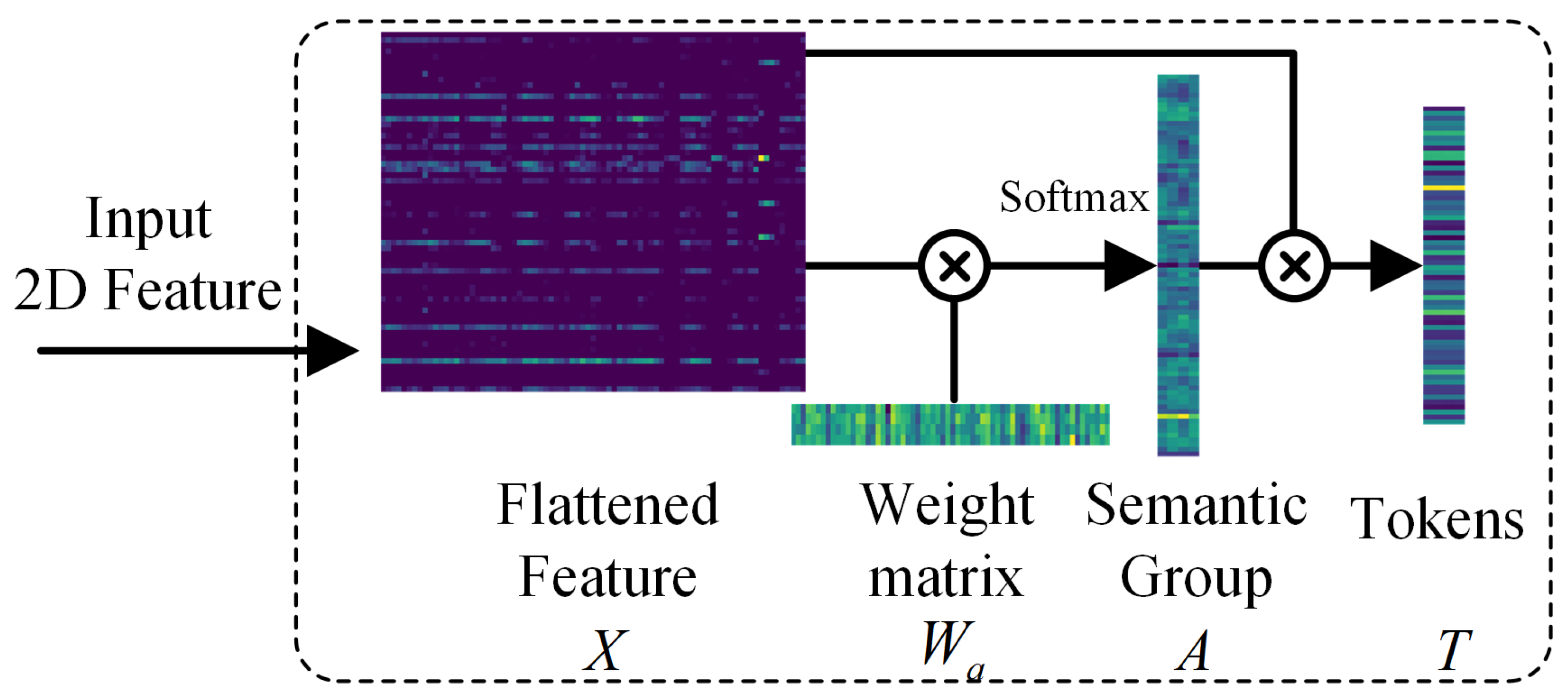
The training samples extract rich shallow spectral–spatial features using the dual-branch CNNs that we designed. However, there is still deeper feature information to be explored. To address this issue, we redefine the obtained shallow spectral–spatial features as semantic tokens. We represent the flattened feature map from the input (obtained by flattening the 2D feature map) as F R u v × z , where u v represents the height and width of the 2D feature map, and z represents the number of channels. The final output obtained by this module is represented as T R t × z , where t is the token number. To obtain feature tokens T from the feature map F , one can use the following equation:
T = s o f t m a x F W a Q T F
In the formula, F W a represents element-wise multiplication with dimensions 1 × 1 , and W a R z × t represents a weight matrix. We initialize this weight matrix using a Gaussian distribution. At this stage, the newly generated semantic groups are represented by Q R u v × t . Next, Q is transposed. We apply the softmax function ( softmax ( · ) ) to the transposed result to emphasize important semantic components. Finally, the multiplication of Q and F generates the module’s final output semantic tokens T . The specific process is visualized in Figure 2.

2.3. Large-Kernel Attention

The tokens output from the previous module can be represented as [ T 1 , T 2 , , T k ] . To make our model more suitable for our classification task, we include a learnable classification token T 0 c l s in the first position of these tokens. In order to not lose the positional information inherent in the image, we embed positional information P E p o s into each semantic token. For T 0 c l s , T 1 , , T k and P E p o s , the input T i n for the Large-Kernel Attention can be represented by the following equation:
T i n = T 0 c l s , T 1 , , T k + P E p o s
In the realm of academic research focused on HSI processing, Large-Kernel Attention offers several valuable contributions to subsequent Transformer modules. First and foremost, it elevates the quality of feature extraction, enhancing the Transformer’s comprehension of image data and thereby advancing overall model performance. Significantly, Large-Kernel Attention serves to alleviate the computational complexity of attention mechanisms, particularly evident when dealing with extensive image datasets, as it effectively reduces the number of positional elements that necessitate consideration, ultimately enhancing computational efficiency. Furthermore, it effectively mitigates the impact of redundant information, thereby fortifying the robustness of the Transformer model. This is especially pertinent within the context of image data processing, given the inherent wealth of information typically contained therein. Lastly, Large-Kernel Attention plays a pivotal role in augmenting computational efficiency, facilitating accelerated model training convergence, and curtailing memory and computational requisites. These advantages collectively position Large-Kernel Attention as an invaluable component within the Transformer architecture for scholarly endeavors in HSI processing.
As depicted in Figure 1, this module primarily consists of a 2D convolution layer with 4 @ 3 × 3 kernels, a dilated 2D convolution layer, and a 2D convolution layer with 4 @ 1 × 1 kernels. The process can be expressed by the following equations:
T i n = ( C o n v 2 D ( D i l a t e d C o n v 2 D ( ( C o n v 2 D ( T i n , k 1 , p 1 ) , k 2 , p 2 , d 1 ) ) , k 3 ) ) T i n
where k represents the size of the convolution kernel, k 1 and k 2 are ( 3 × 3 ) , k 3 is (1 × 1), p represents the fill size, p 1 is (1 × 1), p 2 is (3 × 3), d represents the size of dilation, and d 1 is 3.

2.4. Transformer Encoder Module

After the Large-Kernel Attention, we obtain enhanced quality features, which are then fed into the TE module. This module uses self-attention mechanisms to handle relationships between tokens, capturing both global and local features. As can be observed from Figure 1, this module primarily consists of four components, including two Layer Normalization (LN) layers, a Multilayer Perceptron (MLP) layer, and a Multi-Head Self-Attention (MHSA) block. To facilitate deep neural network training and optimization, alleviate gradient vanishing problems, and enhance performance, residual connections are added after the MHSA block and MLP layer.
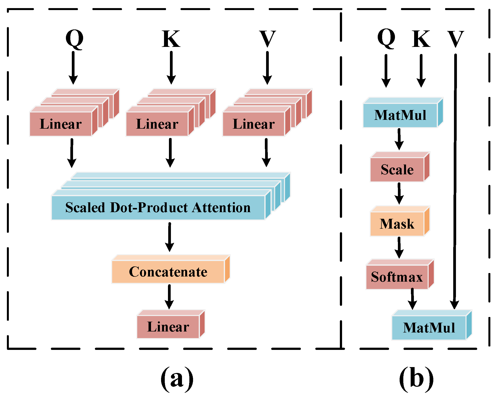
The TE module includes two normalization layers placed before MHSA and MLP, which help alleviate gradient explosion, reduce vanishing gradient problems, and accelerate training. The core of TE is the MHSA block. MHSA integrates the Self-Attention (SA) mechanism, with its essential components typically named Q (Queries), K (Keys), and V (Values). These three matrices are learned during the model’s training process to adapt to the classification task and HSI data. The SA mechanism computes attention scores using Q and K , and the weights of these scores are determined using the softmax function. Subsequently, the scores are multiplied by V to obtain the output of SA, as shown in Figure 3b. These descriptions can be expressed by the following equations:
S A ( Q , K , V ) = s o f t m a x Q K T d K V
where K T is the transpose of K and d K is the dimension of K .
Compared to SA, MHSA uses multiple sets of weight matrices, allowing it to map multiple sets of Q , K , and V . Following the same operations as described earlier, it computes attention values for each set to calculate Multi-Head Attention values. The attention results from each head are then concatenated together. The final step involves concatenating each attention value and multiplying it with the weight matrix W R n × w K × w d , where n represents the number of attention heads and w d represents the number of tokens. The computation equation for MHSA can be expressed as follows:
M H S A ( Q , K , V ) = C o n c a t S A 1 , S A 2 , , S A h W
The MLP component consists of two fully connected layers. After passing through the TE module, T i n is transformed into T o u t . We extract the classification token vector T ^ 0 c l s embedded in Equation (3) for the classification task. Next, we use a linear layer with an output dimension equal to the number of land cover classes in the HSI data. Finally, we use the softmax function to assign the label of the input sample to the category represented by the class with the highest probability in the final vector.
The complete procedure of the ETLKA method, as proposed, is outlined in Algorithm 1.
Algorithm 1 Enhanced Transformer with Large-Kernel Attention Model
Input: Input HSI data P R c × v × e and ground truth labels Y R c × v ; Set the spectral dimension after PCA preprocessing to b = 30 ; Extract patch size s = 13 ; and specify the training sample rate as μ .
Output: Predicted labels for the test dataset.
 1:
Configure batch size = 64, use the Adam optimizer with a learning rate of 5 × 10 4 , and set the number of iterations to ϵ = 150 .
 2:
Obtain PCA-transformed HSI, denoted as P pca , from which generate patches for all samples and split them into training and test sets according to the training sample rate.
 3:
Create training and test data loaders.
 4:
for  i = 1 to ϵ  do
 5:
  Generate shallow features using the spectral–spatial shallow feature extraction module.
 6:
  Flatten the extracted 2D shallow spectral–spatial feature maps to obtain a 1D feature vector.
 7:
  Execute tokenization transformation using feature vectors and initialized weights to produce semantic tokens.
 8:
  The first position of the semantic token sequence combines with a learnable class token, and positional embeddings are applied to these semantic tokens.
 9:
  Perform Large-Kernel Attention and TE module
10:
  Input the learnable class tokens into a linear layer and use the softmax function to obtain classification probabilities.
11:
end for
12:
Use the trained model with the test dataset to obtain predicted labels.

3. Results

3.1. Data Description

The proposed method was tested on three classical HSI datasets, including the Indian Pines dataset, the Pavia University dataset, and the Houston2013 dataset.
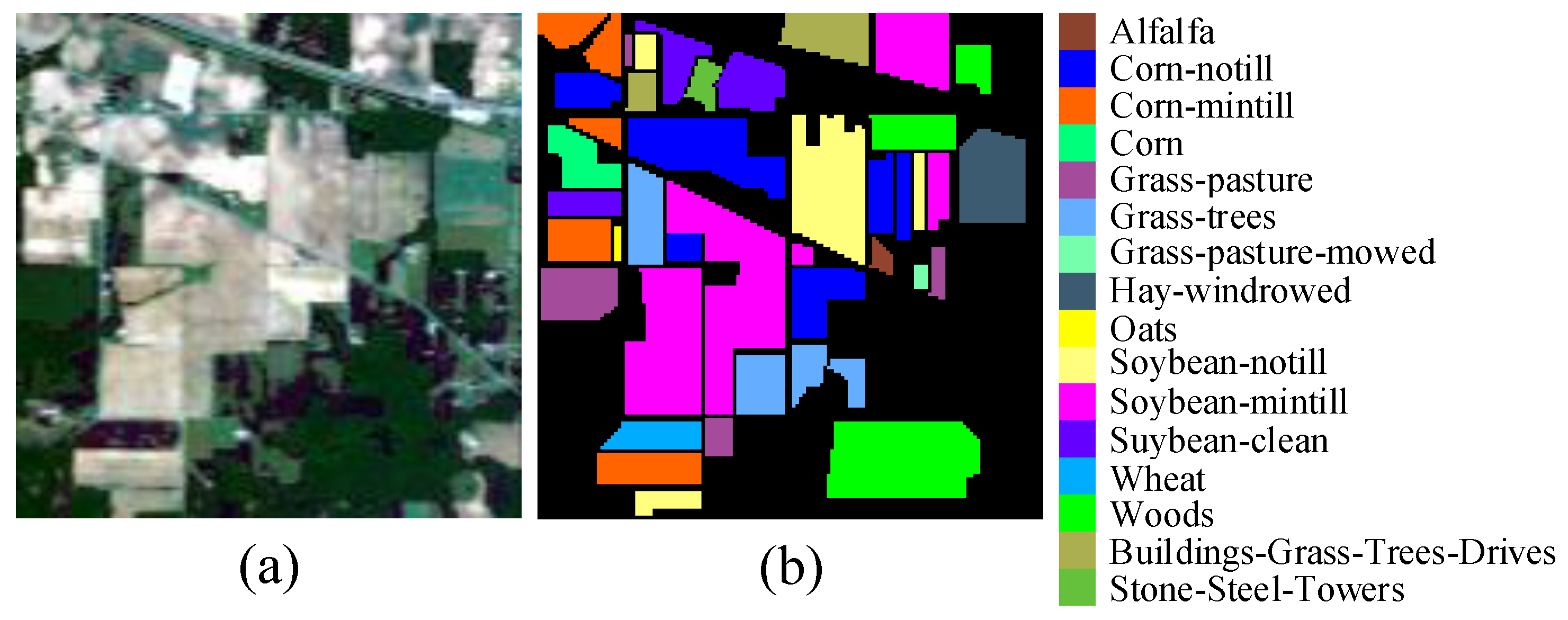
Indian Pines dataset: This dataset was acquired in northwestern Indiana, USA, in 1992, using the Airborne Visible/Infrared Imaging Spectrometer (AVIRIS) sensor. The HSI consists of 224 bands with a wavelength range from 0.4 to 2.5 micrometers. The image comprises 145 × 145 pixels with a spatial resolution of 20 m and includes 16 land cover categories. In our experiments, a total of 200 bands were chosen (excluding water-absorbing and noisy bands). Pseudo-color images and ground-truth maps are illustrated in Figure 4a and b, respectively.
Pavia University dataset: This dataset was captured in 2001 over the University of Pavia in the northern part of Italy using the Reflective Optics System Imaging Spectrometer (ROSIS) sensor. The dataset is an HSI comprising 115 bands with a wavelength ranging from 0.43 to 0.86 micrometers. The image has dimensions of 610 × 340 pixels with a spatial resolution of 1.3 m. It includes 9 land cover categories. In the experiments, 103 bands were selected for analysis, and 12 noisy bands were removed. Pseudo-color images and ground-truth classification maps are displayed in Figure 5a,b.
Houston2013 dataset: This dataset was provided by two organizations, one being the Hyperspectral Imaging Group at the University of Houston, and the other being the National Center for Airborne Laser Mapping (NCALM), funded by the National Science Foundation (NSF). The dataset includes 15 land cover categories. It is a hyperspectral image consisting of 144 bands with a wavelength range from 0.38 to 1.05 micrometers. The dataset comprises 349 × 1905 pixels with a spatial resolution of 2.5 m. Pseudo-color images and ground-truth classification maps are shown in Figure 6a,b.
The land cover category names, number of training samples, and number of test samples regarding these three datasets are listed in Table 1. Each dataset takes 3 % of the samples as the training set and the rest as the test set.

3.2. Parameter Analysis

We analyzed several crucial hyperparameters that have a significant impact on both the classification performance and the training process. These parameters encompass the patch size and the batch size.
(1) Patch Size: To empirically study the effect of patch size, we kept a fixed set of values for the remaining hyperparameters. The patch size was systematically chosen from a predetermined set of candidate values, namely, { 9 , 11 , 13 , 15 , 17 }. Figure 7 shows the effect of different patch sizes on the OA. An optimal OA was achieved in three datasets when the patch size was set to 13.
(2) Batch Size: In Figure 8, the impact of batch size on OA of the three datasets is presented. The batch size was chosen from a set of candidates { 16 , 32 , 64 , 128 , 256 }. Clearly, the classification metrics we have presented achieve the best results when the batch size is set to 64.

3.3. Classification Results and Analysis

At this stage, we conducted comparative experiments with several advanced traditional and deep learning methods to validate the effectiveness and superiority of the proposed ETLKA model. They are SVM [21], EMAP [17], 1D-CNN [33], 2D-CNN [34], 3D-CNN [36], HybridSN [37], and SSFTT [50]. For the listed comparative methods, the network parameters and training strategies in the original paper remain unchanged in the experiments. The number of training and testing samples for the above methods is as shown in Table 1. To ensure a fair comparison, samples are randomly selected.
(1) Quantitative Results and Analysis: In Table 2, Table 3 and Table 4, we present the superiority of the proposed ETLKA method over each of the comparison methods on the Indian Pines, Pavia University, and Houston2013 datasets in four aspects: Overall Accuracy (OA), Average Accuracy (AA), kappa coefficient ( κ ), and class-wise accuracy. OA, AA and κ can be obtained from the following equations:
O A = T P + T N T P + T N + F P + F N
A A = 1 C i = 1 C T P i T P i + F P i
κ = p o p e 1 p e
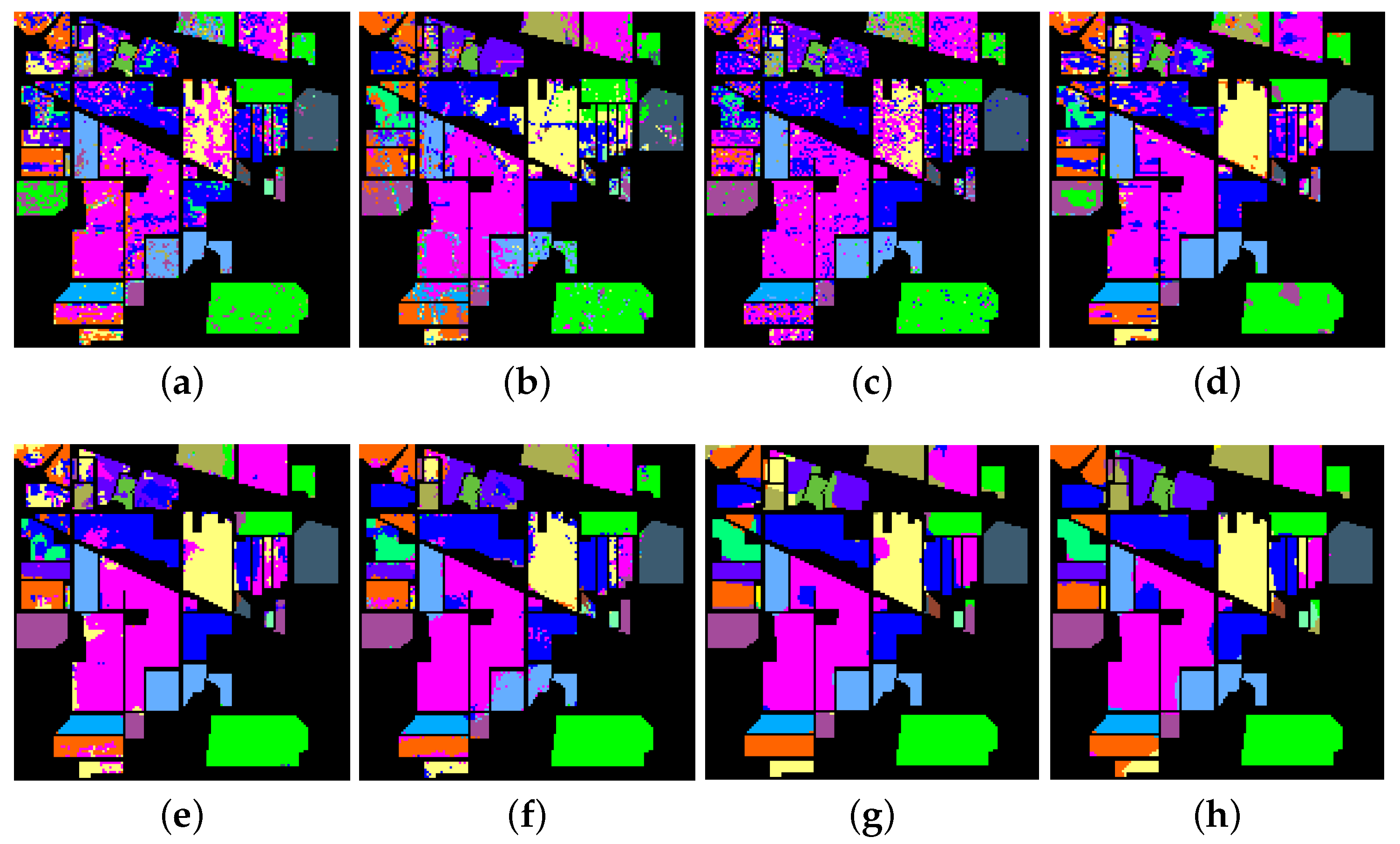
where T P is truly positive, T N is truly negative, F P is false positive, F N is false negative, C is the number of classes, and T P i and F P i are the true positives and false positives for class i, respectively. Additionally, p o is observed accuracy and p e is random accuracy. In classification problems, p o can be calculated through OA, while p e can be calculated through the marginal probabilities of the classes. The best results for each metric in the tables are highlighted in bold. It is evident that our proposed ETLKA model outperforms the seven compared methods. Taking the India Pines dataset as an example, our proposed approach demonstrated superior classification performance for categories ‘Alfalfa’, ‘Corn-min-till’, ‘Corn’, ‘Grass-tree’, ‘Grass-pasture-mowed’, ‘Oats’, ‘Soybean-clean’, and ‘woods’. This owes to the innovative feature extraction method, efficient attention strategy, and the incorporation of the Transformer architecture in our proposed framework. In Figure 9, we visualized the performance comparison of different methods on different datasets. It is evident from the visualization that the proposed ETLKA model exhibits the best performance.
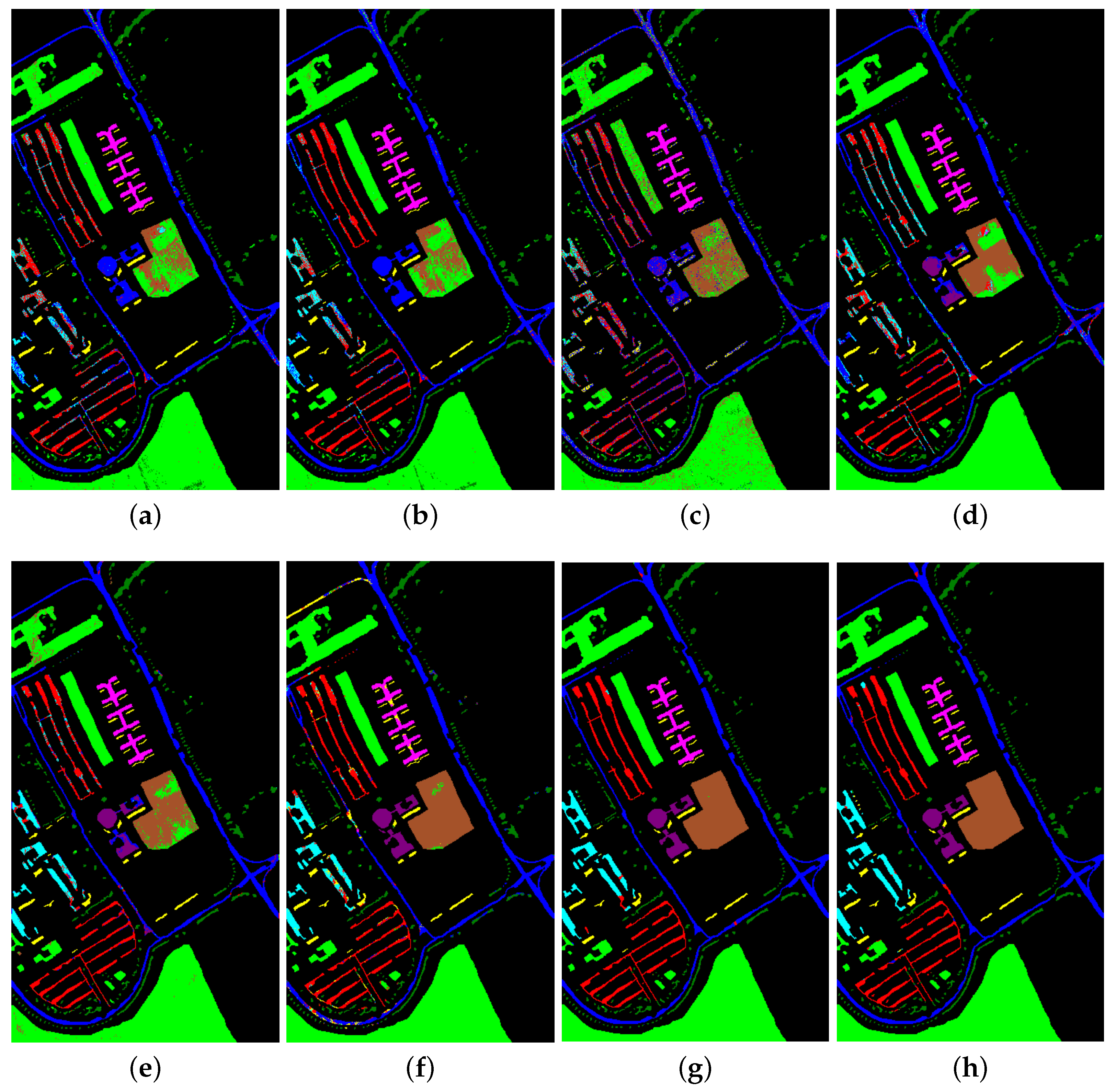
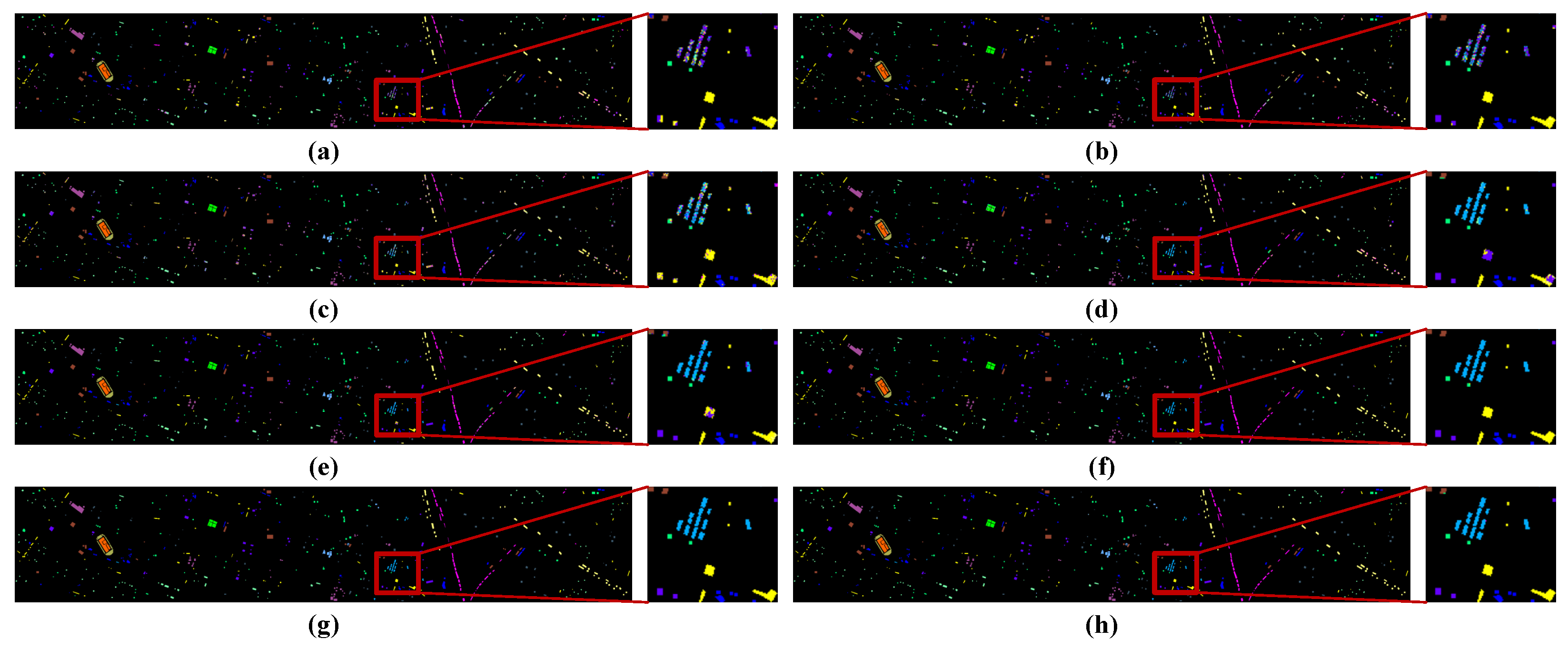
(2) Visual Evaluation and Analysis: Our proposed method, as illustrated in Figure 10, Figure 11 and Figure 12, generated classification maps for three datasets. By comparing these maps in terms of spatial characteristics, edge contours, and the presence of noise, it is clear that our method’s visual maps closely resemble the actual ground-truth maps. In contrast, traditional classifiers generally performed less effectively in comparison to deep learning classifiers, with their classification maps displaying a higher degree of misclassification and noticeable noise.
For 1D-CNN, 2D-CNN, 3D-CNN, and HybridSN methods, while misclassification was reduced, noise outliers were still present. Our method notably mitigated noise-related issues in the classification maps and accurately represented the shapes of the classified regions. In the case of Transformer-based methods, such as SSFTT, the consideration of global information interaction further improved classification accuracy and led to clearer delineation of classification map boundaries. However, our method’s classification maps showed the fewest instances of misclassification and noise, affirming its superior visual classification performance at the same sampling rate. Specifically, in the Indian Pines dataset, various methods performed relatively poorly in classifying categories ’Alfalfa,’ ’Corn,’ and ’Oats.’ Our method achieved highly accurate results. In the Pavia University dataset, two traditional methods exhibited pronounced misclassification in the ’Bitumen’ category region, while other methods displayed more noise in the ’Bare soil’ category. Our method had the fewest classification errors in the ’Bare soil’ category region. For the Houston2013 dataset, the classification results of Transformer-based methods significantly outperformed traditional methods and other deep learning methods.
In summary, visual comparisons across multiple classifiers confirm the outstanding classification performance of our proposed method.

3.4. Inference Speed Analysis

As shown in Table 5, with the epoch set to 150 and the batch size set to 64, we made corresponding records of the network’s training time and testing time. The experimental results indicated that the network exhibited fast inference speed.

3.5. Ablation Analysis

To comprehensively demonstrate the effectiveness of our proposed method, we conducted ablation experiments on the Indian Pines dataset, analyzing the impact of different components on the overall model. As shown in Table 6, we considered four combinations and evaluated their impact on OA, AA, and κ .
Specifically, the complete model was divided into four components, including the Spectral–Spatial Feature Extraction module (SSFE) comprising a dual-branch structure of 3D and 2D convolutional layers, the Tokenizer, LKA, and the TE Module. Notably, when we replaced the Spectral–Spatial Shallow Feature Extraction module with a single 2D convolution layer, the overall accuracy decreased by 1.42%. In the second combination experiment, removing TE resulted in a 2.64% decrease in overall accuracy, with a significant decline in average accuracy. The third combination experiment involved transitioning from parallel 3D–2D convolution layers to a serial arrangement, while removing the LKA module led to a 0.42% decrease in overall accuracy and a substantial 2.88% reduction in average accuracy. In the final experiment, only retaining the Spectral–Spatial Shallow Feature Extraction module caused an average accuracy decrease of 4.21%. This underscores the positive impact of the Transformer architecture on performance enhancement.
In summary, a comprehensive analysis of these combination experiment results further substantiates the effectiveness of our model.

4. Conclusions

This paper introduces a network that utilizes a Transformer architecture with a Large-Kernel Attention Module to deeply extract spatial and spectral information from HSIs, significantly improving classification accuracy. In the spectral–spatial shallow feature extraction stage, we employed a dual-branch structure. The first branch primarily utilized 3D convolution to extract spectral–spatial features from the HSI data, while the second branch used 2D convolution to extract spatial features from the HSI data. Before the Transformer Encoder, we developed a Large-Kernel Attention Module, with the objective of improving the quality of feature extraction. This enhancement leads to a better understanding of image data by the Transformer, resulting in an overall improvement in the model’s performance. Additionally, it effectively mitigates the impact of redundant information, strengthening the robustness of the Transformer model. Experimental evaluations were conducted on three hyperspectral imaging datasets, comparing this approach with existing classification methods. The results confirm the method’s effectiveness and superiority. Future research can focus on the design of an end-to-end lightweight Transformer architecture and leverage a multi-scale feature extraction network to extract diverse feature types, enabling deep exploration of rich feature information in hyperspectral images for further accuracy improvement.

Author Contributions

Conceptualization, W.L. and L.S.; methodology, W.L. and X.W.; software, X.W.; validation, L.S.; investigation, W.L. and X.W.; writing—original draft preparation, X.W.; writing—review and editing, L.S. and Y.Z.; visualization, X.W.; supervision, Y.Z. and L.S.; funding acquisition, W.L. All authors have read and agreed to the published version of the manuscript.

Funding

This research was funded by the National Natural Science Foundation of China, grant number 62076137.

Data Availability Statement

The data presented in this study are available in the article.

Acknowledgments

The authors thank the anonymous reviewers and the editors for their insightful comments and helpful suggestions that helped improve the quality of our manuscript.

Conflicts of Interest

The authors declare no conflicts of interest.

Abbreviations

The following abbreviations are used in this manuscript:
AAAverage Accuracy
EMAPExtended Multiple Attribute Profile
HSIHyperspectral image
LKALarge-Kernal Attention
LNNormalization layers
κ Kappa coefficient
MHSAMulti-Head Self-Attention
OAOverall Accuracy
PCAPrincipal Component Analysis
SVMSupport Vector Machine
TETransformer Encoder

References

  1. Li, J.; Zheng, K.; Liu, W.; Li, Z.; Yu, H.; Ni, L. Model-Guided Coarse-to-Fine Fusion Network for Unsupervised Hyperspectral Image Super-Resolution. IEEE Geosci. Remote Sens. Lett. 2023, 20, 1–5. [Google Scholar] [CrossRef]
  2. Li, J.; Zheng, K.; Li, Z.; Gao, L.; Jia, X. X-Shaped Interactive Autoencoders with Cross-Modality Mutual Learning for Unsupervised Hyperspectral Image Super-Resolution. IEEE Trans. Geosci. Remote Sens. 2023, 61, 1–17. [Google Scholar] [CrossRef]
  3. Sun, L.; Cheng, S.; Zheng, Y.; Wu, Z.; Zhang, J. SPANet: Successive pooling attention network for semantic segmentation of remote sensing images. IEEE J. Sel. Top. Appl. Earth Obs. Remote Sens. 2022, 15, 4045–4057. [Google Scholar] [CrossRef]
  4. García, J.L.; Paoletti, M.E.; Jiménez, L.I.; Haut, J.M.; Plaza, A. Efficient semantic segmentation of hyperspectral images using adaptable rectangular convolution. IEEE Geosci. Remote Sens. Lett. 2022, 19, 1–5. [Google Scholar] [CrossRef]
  5. Ben-Ahmed, O.; Urruty, T.; Richard, N.; Fernandez-Maloigne, C. Toward content-based hyperspectral remote sensing image retrieval (CB-HRSIR): A preliminary study based on spectral sensitivity functions. Remote Sens. 2019, 11, 600. [Google Scholar] [CrossRef]
  6. Sun, L.; Wang, Q.; Chen, Y.; Zheng, Y.; Wu, Z.; Fu, L.; Jeon, B. CRNet: Channel-enhanced Remodeling-based Network for Salient Object Detection in Optical Remote Sensing Images. IEEE Trans. Geosci. Remote Sens. 2023, 61, 5618314. [Google Scholar] [CrossRef]
  7. Fu, L.; Zhang, D.; Ye, Q. Recurrent thrifty attention network for remote sensing scene recognition. IEEE Trans. Geosci. Remote Sens. 2020, 59, 8257–8268. [Google Scholar] [CrossRef]
  8. Ren, H.; Du, Q.; Wang, J.; Chang, C.I.; Jensen, J.O.; Jensen, J.L. Automatic target recognition for hyperspectral imagery using high-order statistics. IEEE Trans. Aerosp. Electron. Syst. 2006, 42, 1372–1385. [Google Scholar] [CrossRef]
  9. Matteoli, S.; Diani, M.; Corsini, G. A tutorial overview of anomaly detection in hyperspectral images. IEEE Aerosp. Electron. Syst. Mag. 2010, 25, 5–28. [Google Scholar] [CrossRef]
  10. Li, L.; Li, W.; Qu, Y.; Zhao, C.; Tao, R.; Du, Q. Prior-based tensor approximation for anomaly detection in hyperspectral imagery. IEEE Trans. Neural Netw. Learn. Syst. 2020, 33, 1037–1050. [Google Scholar] [CrossRef]
  11. Pedergnana, M.; Marpu, P.R.; Mura, M.D.; Benediktsson, J.A.; Bruzzone, L. A Novel Technique for Optimal Feature Selection in Attribute Profiles Based on Genetic Algorithms. IEEE Trans. Geosci. Remote Sens. 2013, 51, 3514–3528. [Google Scholar] [CrossRef]
  12. Song, B.; Li, J.; Dalla Mura, M.; Li, P.; Plaza, A.; Bioucas-Dias, J.M.; Benediktsson, J.A.; Chanussot, J. Remotely Sensed Image Classification Using Sparse Representations of Morphological Attribute Profiles. IEEE Trans. Geosci. Remote Sens. 2014, 52, 5122–5136. [Google Scholar] [CrossRef]
  13. Xia, J.; Dalla Mura, M.; Chanussot, J.; Du, P.; He, X. Random Subspace Ensembles for Hyperspectral Image Classification with Extended Morphological Attribute Profiles. IEEE Trans. Geosci. Remote Sens. 2015, 53, 4768–4786. [Google Scholar] [CrossRef]
  14. Kwan, C.; Gribben, D.; Ayhan, B.; Bernabe, S.; Plaza, A.; Selva, M. Improving Land Cover Classification Using Extended Multi-Attribute Profiles (EMAP) Enhanced Color, Near Infrared, and LiDAR Data. Remote Sens. 2020, 12, 1392. [Google Scholar] [CrossRef]
  15. Kwan, C.; Ayhan, B.; Budavari, B.; Lu, Y.; Perez, D.; Li, J.; Bernabe, S.; Plaza, A. Deep Learning for Land Cover Classification Using Only a Few Bands. Remote Sens. 2020, 12, 2000. [Google Scholar] [CrossRef]
  16. Zhang, A.; Sun, G.; Ma, P.; Jia, X.; Ren, J.; Huang, H.; Zhang, X. Coastal Wetland Mapping with Sentinel-2 MSI Imagery Based on Gravitational Optimized Multilayer Perceptron and Morphological Attribute Profiles. Remote Sens. 2019, 11, 952. [Google Scholar] [CrossRef]
  17. Huang, J.; Liu, K.; Xu, M.; Perc, M.; Li, X. Background Purification Framework With Extended Morphological Attribute Profile for Hyperspectral Anomaly Detection. IEEE J. Sel. Top. Appl. Earth Obs. Remote Sens. 2021, 14, 8113–8124. [Google Scholar] [CrossRef]
  18. Ye, Q.; Huang, P.; Zhang, Z.; Zheng, Y.; Fu, L.; Yang, W. Multiview learning with robust double-sided twin SVM. IEEE Trans. Cyber. 2021, 52, 12745–12758. [Google Scholar] [CrossRef]
  19. Fu, L.; Li, Z.; Ye, Q.; Yin, H.; Liu, Q.; Chen, X.; Fan, X.; Yang, W.; Yang, G. Learning Robust Discriminant Subspace Based on Joint L2, p-and L2, s-Norm Distance Metrics. IEEE Trans. Neural Netw. Learn. Syst. 2020, 33, 130–144. [Google Scholar] [CrossRef]
  20. Ye, Q.; Li, Z.; Fu, L.; Zhang, Z.; Yang, W.; Yang, G. Nonpeaked discriminant analysis for data representation. IEEE Trans. Neural Netw. Learn. Syst. 2019, 30, 3818–3832. [Google Scholar] [CrossRef]
  21. Baassou, B.; He, M.; Mei, S. An accurate SVM-based classification approach for hyperspectral image classification. In Proceedings of the 2013 21st International Conference on Geoinformatics, Kaifeng, China, 20–22 June 2013; pp. 1–7. [Google Scholar]
  22. Guo, B.; Gunn, S.R.; Damper, R.I.; Nelson, J.D. Customizing kernel functions for SVM-based hyperspectral image classification. IEEE Trans. Image Proc. 2008, 17, 622–629. [Google Scholar] [CrossRef] [PubMed]
  23. Melgani, F.; Bruzzone, L. Classification of hyperspectral remote sensing images with support vector machines. IEEE Trans. Geosci. Remote Sens. 2004, 42, 1778–1790. [Google Scholar] [CrossRef]
  24. Kang, X.; Xiang, X.; Li, S.; Benediktsson, J.A. PCA-based edge-preserving features for hyperspectral image classification. IEEE Trans. Geosci. Remote Sens. 2017, 55, 7140–7151. [Google Scholar] [CrossRef]
  25. Wang, F.; Zhang, R.; Wu, Q. Hyperspectral image classification based on PCA network. In Proceedings of the 2016 8th Workshop on Hyperspectral Image and Signal Processing: Evolution in Remote Sensing (WHISPERS), Los Angeles, CA, USA, 21–24 August 2016; pp. 1–4. [Google Scholar]
  26. Villa, A.; Benediktsson, J.A.; Chanussot, J.; Jutten, C. Hyperspectral image classification with independent component discriminant analysis. IEEE Trans. Geosci. Remote Sens. 2011, 49, 4865–4876. [Google Scholar] [CrossRef]
  27. Bandos, T.V.; Bruzzone, L.; Camps-Valls, G. Classification of hyperspectral images with regularized linear discriminant analysis. IEEE Trans. Geosci. Remote Sens. 2009, 47, 862–873. [Google Scholar] [CrossRef]
  28. Su, Y.; Gao, L.; Jiang, M.; Plaza, A.; Sun, X.; Zhang, B. NSCKL: Normalized Spectral Clustering With Kernel-Based Learning for Semisupervised Hyperspectral Image Classification. IEEE Trans. Cybern. 2023, 53, 6649–6662. [Google Scholar] [CrossRef]
  29. Lee, H.; Kwon, H. Going Deeper With Contextual CNN for Hyperspectral Image Classification. IEEE Trans. Image Process. 2017, 26, 4843–4855. [Google Scholar] [CrossRef]
  30. Sun, L.; Fang, Y.; Chen, Y.; Huang, W.; Wu, Z.; Jeon, B. Multi-structure KELM with attention fusion strategy for hyperspectral image classification. IEEE Trans. Geosci. Remote Sens. 2022, 60, 1–17. [Google Scholar] [CrossRef]
  31. Gao, H.; Yang, Y.; Li, C.; Gao, L.; Zhang, B. Multiscale residual network with mixed depthwise convolution for hyperspectral image classification. IEEE Trans. Geosci. Remote Sens. 2020, 59, 3396–3408. [Google Scholar] [CrossRef]
  32. Gao, H.; Chen, Z.; Xu, F. Adaptive spectral-spatial feature fusion network for hyperspectral image classification using limited training samples. Int. J. Appl. Earth Obs. Geoinf. 2022, 107, 102687. [Google Scholar] [CrossRef]
  33. Hu, W.; Huang, Y.; Wei, L.; Zhang, F.; Li, H. Deep convolutional neural networks for hyperspectral image classification. J. Sens. 2015, 2015, 1–12. [Google Scholar] [CrossRef]
  34. Zhao, W.; Du, S. Spectral–spatial feature extraction for hyperspectral image classification: A dimension reduction and deep learning approach. IEEE Trans. Geosci. Remote Sens. 2016, 54, 4544–4554. [Google Scholar] [CrossRef]
  35. Yang, J.; Zhao, Y.Q.; Chan, J.C.W. Learning and transferring deep joint spectral–spatial features for hyperspectral classification. IEEE Trans. Geosci. Remote Sens. 2017, 55, 4729–4742. [Google Scholar] [CrossRef]
  36. Chen, Y.; Jiang, H.; Li, C.; Jia, X.; Ghamisi, P. Deep feature extraction and classification of hyperspectral images based on convolutional neural networks. IEEE Trans. Geosci. Remote Sens. 2016, 54, 6232–6251. [Google Scholar] [CrossRef]
  37. Roy, S.K.; Krishna, G.; Dubey, S.R.; Chaudhuri, B.B. HybridSN: Exploring 3-D–2-D CNN feature hierarchy for hyperspectral image classification. IEEE Geosci. Remote Sens. Lett. 2019, 17, 277–281. [Google Scholar] [CrossRef]
  38. He, K.; Zhang, X.; Ren, S.; Sun, J. Deep residual learning for image recognition. In Proceedings of the IEEE Conference on Computer Vision and Pattern Recognition, Las Vegas, NV, USA, 26 June–1 July 2016; pp. 770–778. [Google Scholar]
  39. Zhong, Z.; Li, J.; Luo, Z.; Chapman, M. Spectral–spatial residual network for hyperspectral image classification: A 3-D deep learning framework. IEEE Trans. Geosci. Remote Sens. 2017, 56, 847–858. [Google Scholar] [CrossRef]
  40. Paoletti, M.E.; Haut, J.M.; Fernandez-Beltran, R.; Plaza, J.; Plaza, A.J.; Pla, F. Deep pyramidal residual networks for spectral–spatial hyperspectral image classification. IEEE Trans. Geosci. Remote Sens. 2018, 57, 740–754. [Google Scholar] [CrossRef]
  41. Wang, J.; Song, X.; Sun, L.; Huang, W.; Wang, J. A novel cubic convolutional neural network for hyperspectral image classification. IEEE J. Sel. Top. Appl. Earth Obs. Remote Sens. 2020, 13, 4133–4148. [Google Scholar] [CrossRef]
  42. Roy, S.K.; Hong, D.; Kar, P.; Wu, X.; Liu, X.; Zhao, D. Lightweight heterogeneous kernel convolution for hyperspectral image classification with noisy labels. IEEE Geosci. Remote Sens. Lett. 2021, 19, 1–5. [Google Scholar] [CrossRef]
  43. Dosovitskiy, A.; Beyer, L.; Kolesnikov, A.; Weissenborn, D.; Zhai, X.; Unterthiner, T.; Dehghani, M.; Minderer, M.; Heigold, G.; Gelly, S.; et al. An image is worth 16x16 words: Transformers for image recognition at scale. arXiv 2020, arXiv:2010.11929. [Google Scholar]
  44. Carion, N.; Massa, F.; Synnaeve, G.; Usunier, N.; Kirillov, A.; Zagoruyko, S. End-to-end object detection with transformers. In European Conference on Computer Vision; Springer: Cham, Switzerland, 2020; pp. 213–229. [Google Scholar]
  45. Liu, Z.; Lin, Y.; Cao, Y.; Hu, H.; Wei, Y.; Zhang, Z.; Lin, S.; Guo, B. Swin transformer: Hierarchical vision transformer using shifted windows. In Proceedings of the IEEE/CVF International Conference on Computer Vision (CVPR), Nashville, TN, USA, 20–25 June 2021; pp. 10012–10022. [Google Scholar]
  46. Strudel, R.; Garcia, R.; Laptev, I.; Schmid, C. Segmenter: Transformer for semantic segmentation. In Proceedings of the IEEE/CVF International Conference on Computer Vision (CVPR), Nashville, TN, USA, 20–25 June 2021; pp. 7262–7272. [Google Scholar]
  47. Vaswani, A.; Shazeer, N.; Parmar, N.; Uszkoreit, J.; Jones, L.; Gomez, A.N.; Kaiser, Ł.; Polosukhin, I. Attention is all you need. Proc. Adv. Neural Inf. Process. Syst. (NIPS) 2017, 30, 1–11. [Google Scholar]
  48. Yang, X.; Cao, W.; Lu, Y.; Zhou, Y. Hyperspectral Image Transformer Classification Networks. IEEE Trans. Geosci. Remote Sens. 2022, 60, 1–15. [Google Scholar] [CrossRef]
  49. Hong, D.; Han, Z.; Yao, J.; Gao, L.; Zhang, B.; Plaza, A.; Chanussot, J. SpectralFormer: Rethinking hyperspectral image classification with transformers. IEEE Trans. Geosci. Remote Sens. 2021, 60, 1–15. [Google Scholar] [CrossRef]
  50. Sun, L.; Zhao, G.; Zheng, Y.; Wu, Z. Spectral–spatial feature tokenization transformer for hyperspectral image classification. IEEE Trans. Geosci. Remote Sens. 2022, 60, 1–14. [Google Scholar] [CrossRef]
  51. Xue, Z.; Xu, Q.; Zhang, M. Local transformer with spatial partition restore for hyperspectral image classification. IEEE J. Sel. Top. Appl. Earth Observ. Remote Sens. 2022, 15, 4307–4325. [Google Scholar] [CrossRef]
  52. Huang, X.; Dong, M.; Li, J.; Guo, X. A 3-d-swin transformer-based hierarchical contrastive learning method for hyperspectral image classification. IEEE Trans. Geosci. Remote Sens. 2022, 60, 1–15. [Google Scholar] [CrossRef]
  53. Fang, Y.; Ye, Q.; Sun, L.; Zheng, Y.; Wu, Z. Multi-Attention Joint Convolution Feature Representation with Lightweight Transformer for Hyperspectral Image Classification. IEEE Trans. Geosci. Remote Sens. 2023, 61, 1–14. [Google Scholar]
  54. Xu, Y.; Xie, Y.; Li, B.; Xie, C.; Zhang, Y.; Wang, A.; Zhu, L. Spatial-Spectral 1DSwin Transformer with Group-wise Feature Tokenization for Hyperspectral Image Classification. IEEE Trans. Geosci. Remote Sens. 2023, 61, 1–16. [Google Scholar]
  55. Zhang, S.; Zhang, J.; Wang, X.; Wang, J.; Wu, Z. ELS2T: Efficient Lightweight Spectral–Spatial Transformer for Hyperspectral Image Classification. IEEE Trans. Geosci. Remote Sens. 2023, 61, 1–16. [Google Scholar] [CrossRef]
  56. Zhang, K.; Zhu, D.; Min, X.; Zhai, G. Implicit Neural Representation Learning for Hyperspectral Image Super-Resolution. In Proceedings of the 2022 IEEE International Conference on Multimedia and Expo (ICME), Taipei, Taiwan, 18–22 July 2022; pp. 1–6. [Google Scholar] [CrossRef]
  57. Dong, W.; Wang, H.; Wu, F.; Shi, G.; Li, X. Deep Spatial–Spectral Representation Learning for Hyperspectral Image Denoising. IEEE Trans. Comput. Imaging 2019, 5, 635–648. [Google Scholar] [CrossRef]
  58. Tulczyjew, L.; Kawulok, M.; Nalepa, J. Unsupervised Feature Learning Using Recurrent Neural Nets for Segmenting Hyperspectral Images. IEEE Geosci. Remote Sens. Lett. 2021, 18, 2142–2146. [Google Scholar] [CrossRef]
  59. Nalepa, J.; Myller, M.; Imai, Y.; Honda, K.I.; Takeda, T.; Antoniak, M. Unsupervised Segmentation of Hyperspectral Images Using 3-D Convolutional Autoencoders. IEEE Geosci. Remote Sens. Lett. 2020, 17, 1948–1952. [Google Scholar] [CrossRef]
  60. Sellami, A.; Tabbone, S. Deep neural networks-based relevant latent representation learning for hyperspectral image classification. Pattern Recognit. 2022, 121, 108224. [Google Scholar] [CrossRef]
  61. Zhang, S.; Zhang, X.; Li, T.; Meng, H.; Cao, X.; Wang, L. Adversarial Representation Learning for Hyperspectral Image Classification with Small-Sized Labeled Set. Remote Sens. 2022, 14, 2612. [Google Scholar] [CrossRef]
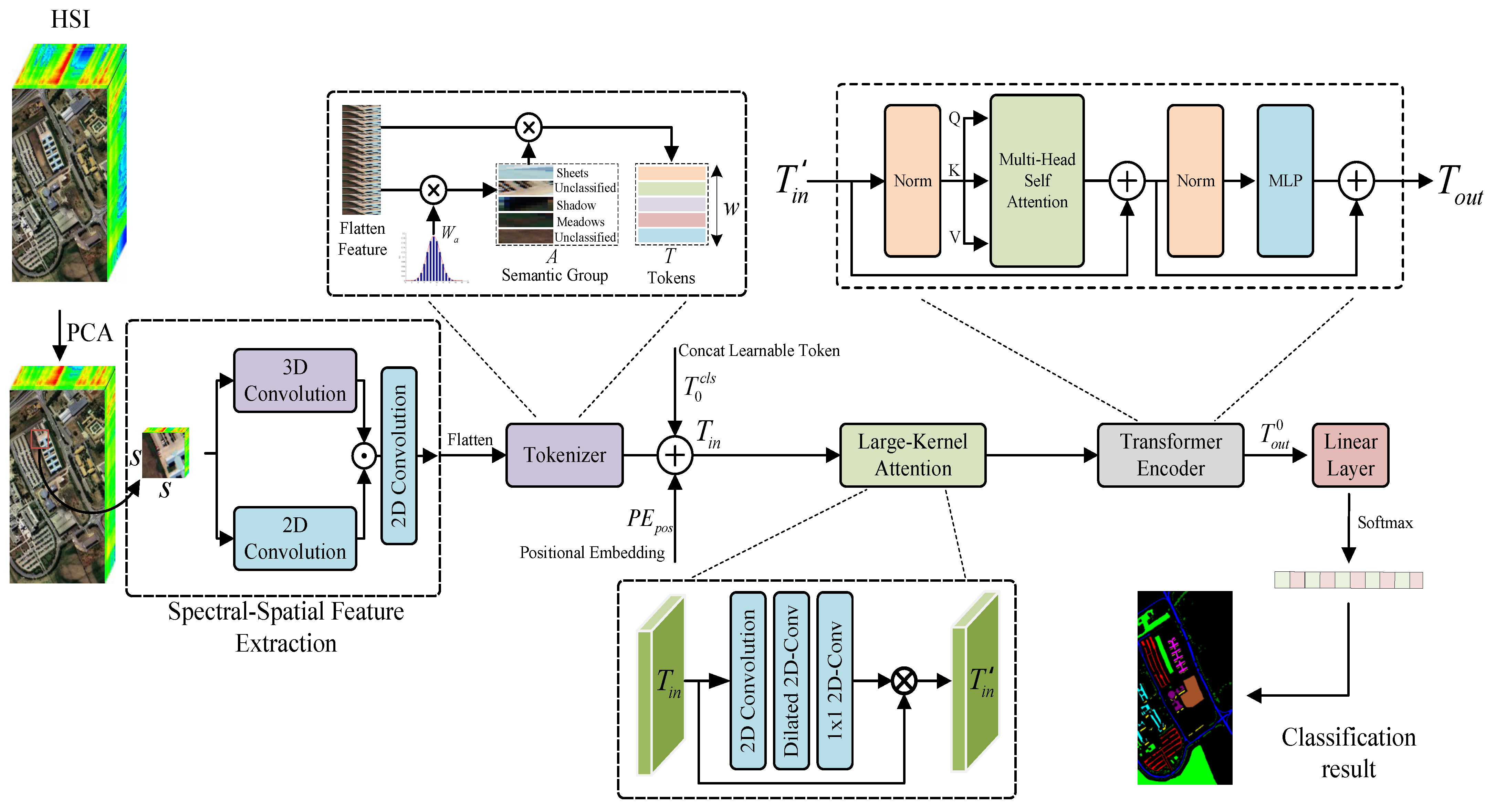
Figure 1. The overall framework of the proposed ETLKA network for the HSI classification.
Remotesensing 16 00067 g001
Figure 2. The visualization process of the HSI Feature Tokenization [50].
Remotesensing 16 00067 g002
Figure 3. Visual representations of (a) Multi-Head Self-Attention Module and (b) self-attention in the Transformer architecture.
Remotesensing 16 00067 g003
Figure 4. Visualization of the India Pines (IP) dataset. (a) Pseudo-color image for the dataset. (b) Ground-truth map for the dataset.
Remotesensing 16 00067 g004
Figure 5. Visualization of the Pavia University (PU) dataset. (a) Pseudo-color image for the dataset. (b) Ground-truth map for the dataset.
Remotesensing 16 00067 g005
Figure 6. Visualization of the Houston2013 dataset. (a) Pseudo-color image for the dataset. (b) Ground-truth map for the dataset.
Remotesensing 16 00067 g006
Figure 7. The impact of different patch sizes on Overall Accuracy, Average Accuracy, and kappa coefficient. (a) India Pines dataset, (b) Pavia University dataset, (c) Houston2013 dataset.
Remotesensing 16 00067 g007
Figure 8. The impact of different batch sizes on Overall Accuracy, Average Accuracy, and kappa coefficient. (a) India Pines dataset, (b) Pavia University dataset, (c) Houston2013 dataset.
Remotesensing 16 00067 g008
Figure 9. The overall visualization presents the performance of different methods on various datasets. (a) India Pines dataset, (b) Pavia University dataset, (c) Houston2013 dataset.
Remotesensing 16 00067 g009
Figure 10. Classification maps of Indian Pines dataset. (a) SVM, (b) EMAP, (c) 1D-CNN, (d) 2D-CNN, (e) 3D-CNN, (f) HybridSN, (g) SSFTT, (h) Proposed.
Remotesensing 16 00067 g010
Figure 11. Classification maps of Pavia University dataset. (a) SVM, (b) EMAP, (c) 1D-CNN, (d) 2D-CNN, (e) 3D-CNN, (f) HybridSN, (g) SSFTT, (h) Proposed.
Remotesensing 16 00067 g011
Figure 12. Classification maps of Houston2013 dataset. (a) SVM, (b) EMAP, (c) 1D-CNN, (d) 2D-CNN, (e) 3D-CNN, (f) HybridSN, (g) SSFTT, (h) Proposed.
Remotesensing 16 00067 g012
Table 1. Training and test sample numbers in the India Pines dataset, Pavia University dataset, and Houston2013 dataset.
NO.India PinesPavia UniversityHouston2013
ClassTrainingTestClassTrainingTestClassTrainingTest
#1Alfalfa145Asphalt1996432Healthy Grass1251126
#2Corn-notill431385Meadows55918,090Stressed Grass1251129
#3Corn-mintill25805Gravel632036Synthetis Grass70627
#4Corn7230Trees922972Tree1241120
#5Grass-pasture14469Metal Sheets401305Soil1241118
#6Grass-tree22708Bare soil1514878Water33292
#7Grass-pasture-mowed127Bitumen401290Residential1271141
#8Hay-windrowed14464Bricks1113571Commercial1241120
#9Oats119Shadows28919Road1251127
#10Soybean-notill29943 Highway1231104
#11Soybean-mintill732382 Railway1231112
#12Soybean-clean18575 Parking Lot 11231110
#13wheat6199 Parking Lot 247422
#14woods381227 Tennis Court43385
#15Buildings-Grass-Trees12374 Running Track66594
#16Stone-Steel-Towers390
Total3079942Total128314,493Total150213,527
Table 2. Different methods exhibit various classification metrics on the Indian Pines dataset. The optimal results are bolded.
NO.SVM [21]EMAP [17]1D-CNN [33]2D-CNN [34]3D-CNN [36]HybridSN [37]SSFTT [50]Proposed
122.2217.0711.6817.4646.1334.0948.0078.67
262.3170.5581.8768.4675.8491.9692.7491.89
349.6870.0119.4166.5463.5079.5986.5593.90
417.8266.1920.3940.1844.3764.0088.9698.35
544.7774.2577.1366.6796.5194.1288.3284.14
686.5861.3494.0497.5498.8690.6298.8099.00
788.8960.0046.6767.0470.3785.1994.8197.04
895.0482.3297.2998.3799.4597.8098.1597.16
910.5320.4511.7615.2626.3268.4288.4297.37
1047.0871.8932.9284.0685.3684.7295.2688.12
1171.9980.9983.7685.7193.4896.7895.5496.56
1230.9863.1148.6148.6764.6578.1587.4390.19
1394.9793.4693.1098.9798.9795.3899.8596.68
1492.7587.0991.6389.0996.9298.9297.4798.22
1515.7764.8442.0755.0470.5785.8393.5094.97
1693.3369.0572.1571.2674.7185.2396.4494.11
OA (%)64.3973.5864.8377.8184.5990.5793.8194.23
AA (%)57.1764.6155.6664.5772.9583.1890.6493.52
κ  × 10059.0769.8762.7474.5682.2689.1792.9493.43
Table 3. Different methods exhibit various classification metrics on the Pavia University dataset. The optimal results are bolded.
NO.SVM [21]EMAP [17]1D-CNN [33]2D-CNN [34]3D-CNN [36]HybridSN [37]SSFTT [50]Proposed
183.0587.5079.2788.6492.9587.8497.3999.26
287.3693.3589.3397.7597.8599.8799.8999.78
342.5955.9747.9942.9782.4585.0894.4796.67
481.4785.3679.1092.9895.3791.3894.8697.84
595.1797.4798.9299.3295.6391.5098.6799.74
640.1548.5476.4276.1479.5993.9399.7799.88
714.9228.3920.7063.7876.4489.3899.3899.53
871.2385.1374.1972.1388.0890.3396.2595.21
987.5496.8471.4798.9399.7896.1297.4897.17
OA (%)76.6880.7676.8587.2890.2394.2698.4498.96
AA (%)70.4374.1564.2780.5288.9593.2797.5798.34
κ  × 10074.8779.1169.1582.8489.7293.7397.9498.62
Table 4. Different methods exhibit various classification metrics on the Houston2013 dataset. The optimal results are bolded.
NO.SVM [21]EMAP [17]1D-CNN [33]2D-CNN [34]3D-CNN [36]HybridSN [37]SSFTT [50]Proposed
195.6587.8586.2094.0293.7598.8599.6699.42
297.5292.5395.1396.3094.9199.7399.1499.81
399.8499.84100.0089.7395.5499.8499.6899.79
493.6692.6395.4398.3194.9196.0799.3498.40
598.3097.2698.9897.88100.00100.0099.99100.00
684.2582.1695.1573.4689.86100.0098.1599.73
782.6580.4776.6089.6391.8497.6399.1199.56
856.6170.5158.1280.9680.3697.9598.6199.26
973.9172.6963.1670.9893.5898.6798.7499.26
1083.5186.7855.5784.6594.2899.0099.9999.84
1168.9764.5970.1690.9692.6499.2899.8299.94
1260.7259.1854.7491.4694.3799.4699.6099.19
1325.6945.2941.9385.6590.9798.1096.4999.43
1493.2596.4897.0573.7194.58100.00100.00100.00
1599.6698.4599.0499.5299.6599.49100.0099.70
OA (%)80.9282.3977.6489.0593.7398.8099.3499.51
AA (%)79.6178.4979.1587.8293.5698.9399.2299.56
κ  × 10079.3380.6475.8188.1593.6398.7199.2899.47
Table 5. Inference time analysis on different datasets.
DatasetIndia PinesPavia UniversityHouston2013
TrainTestTrainTestTrainTest
Time (s)8.0971.8526.92276.6532.01100.31
Table 6. Ablation studies on different components for Indian Pines dataset (accuracy in %). The optimal results are bolded.
CasesComponentsTrainableIndicators
SSFETokenizerLKATEParameters (MB)OA (%)AA (%) κ × 100 p(t-Test)
1Only 2D0.1492.8191.9191.810.4834
2×0.7191.5985.1090.410.4780
33D-Conv+2D-Conv×0.5693.8190.6492.940.4846
4×××0.7090.0286.1289.560.4727
50.7794.2393.5293.430.4926
Disclaimer/Publisher’s Note: The statements, opinions and data contained in all publications are solely those of the individual author(s) and contributor(s) and not of MDPI and/or the editor(s). MDPI and/or the editor(s) disclaim responsibility for any injury to people or property resulting from any ideas, methods, instructions or products referred to in the content.