SAR Image Segmentation by Efficient Fuzzy C-Means Framework with Adaptive Generalized Likelihood Ratio Nonlocal Spatial Information Embedded

Abstract

The existence of multiplicative noise in synthetic aperture radar (SAR) images makes SAR segmentation by fuzzy c-means (FCM) a challenging task. To cope with speckle noise, we first propose an unsupervised FCM with embedding log-transformed Bayesian non-local spatial information (LBNL_FCM). This non-local information is measured by a modified Bayesian similarity metric which is derived by applying the log-transformed SAR distribution to Bayesian theory. After, we construct the similarity metric of patches as the continued product of corresponding pixel similarity measured by generalized likelihood ratio (GLR) to avoid the undesirable characteristics of log-transformed Bayesian similarity metric. An alternative unsupervised FCM framework named GLR_FCM is then proposed. In both frameworks, an adaptive factor based on the local intensity entropy is employed to balance the original and non-local spatial information. Additionally, the membership degree smoothing and the majority voting idea are integrated as supplementary local information to optimize segmentation. Concerning experiments on simulated SAR images, both frameworks can achieve segmentation accuracy of over 97%. On real SAR images, both unsupervised FCM segmentation frameworks work well on SAR homogeneous segmentation in terms of region consistency and edge preservation.

1. Introduction

Segmentation is a fundamental problem in SAR image analysis and applications. The primary purpose of segmentation is to segment the image into non-intersecting and consistent regions that are homogeneous [1]. Due to coherent speckle noise, which can be modeled as a powerful multiplicative noise, SAR image segmentation is recognized as a complex task. So far, many SAR image segmentation methods have been proposed to cope with the effect of speckle noise on image segmentation, such as threshold-based method [2], edge-based methods [3], region-based methods [4,5,6,7,8,9], cluster methods [10,11,12,13], Markov random field methods [3,14], Level set methods [15], graph-based methods [16,17], and deep learning based methods [18,19,20,21]. Among these methods, clustering is a commonly used method in segmentation tasks due to its effectiveness and stability. The fuzzy s-means (FCM) [22] is a classical clustering algorithm and has been extensively used to segment images. Unlike the hard clustering strategy, FCM is a soft clustering algorithm that allocates membership degrees to every category for each pixel. The FCM can achieve a good result for noise-free images. However, the standard FCM is noise-sensitive and lacks robustness without considering any spatial information. Thus, many modified algorithms have been proposed to enhance the effectiveness and robustness of standard FCM against noise.

Ref. Ahmed et al. [23] incorporated the spatial neighborhood term into the objective function of FCM, named BCFCM. BCFCM can modify the label of the center pixel by neighborhood weight distance and enhance the robustness to noise. However, it is time consuming. To reduce the complexity, Ref. Chen and Zhang [24] replaced the spatial neighborhood term with a mean-filtered and median-filtered image, respectively, called FCM_S1 and FCM_S2. Because of the availability of these two images in advance, the time complexity is greatly reduced. Besides, kernel methods were embedded into FCM_S1 and FCM_S2 to explore the non-Euclidean structure of data. Then two kernelized versions, KFCM_S1 and KFCM_S2, were derived. Ref. Szilagyi et al. [25] proposed the enhanced FCM, named EnFCM, which executed clustering on a gray level histogram rather than pixels to reduce the computation cost considerably. Afterwards, the fast generalized FCM (FGFCM) was proposed by Cai et al. [26]. In FGFCM, a new factor $S_{ij}$ was used to measure the local (both spatial and gray) similarity instead of $\alpha$ in EnFCM. The original image and its local spatial and gray level neighborhood are used to construct a non-linear weighted sum image, and then the clustering process is executed on the gray level histogram of the summed image. Thus, the computational load is very light. It is noteworthy that in all the aforementioned algorithms, the parameters for balancing noise immunity and edge preservation are needed. To avoid the parameter selection, Ref. Krinidis and Chatzis [27] introduced a new factor, $G_{ki}$, incorporating local spatial and gray information into the objective function in a fuzzy way and proposed a new FCM named FLICM. This algorithm completely avoids the selection of parameters and is relatively independent of the type of noise.

However, when an image is contaminated with powerful noise, the local information may also be contaminated and unreliable. Actually, for a pixel, plenty of pixels with a similar neighborhood structural configuration exist on the image [28]. Exploring a larger space and incorporating nonlocal spatial information is necessary. Ref. Wang et al. [29] proposed a modified FCM with incorporating both local and non-local spatial information. Ref. Zhu et al. [30] introduced a novel membership constraint and a new objective function was constructed, named GIFP_FCM. Afterwards, Ref. Zhao et al. [31] incorporated non-local information into the objective function of the standard FCM and GIFP_FCM, respectively, and proposed two improved FCMs: An FCM with non-local spatial information (FCM_NLS) [31] and a novel FCM with a non-local adaptive spatial constraint term (FCM_NLASC) [32].

While the improved FCM listed above works well on simulated, nature, and MR images, none of them consider the statistical characteristics of SAR images. Consequently, the above-mentioned methods cannot assure a segmentation result on SAR images. To solve this problem, Ref. Feng et al. [33] proposed a robust non-local FCM with edge preservation (NLEP_FCM). In this algorithm, a modified ratio distance to measure patch similarity for SAR images was defined, and a sum image was constructed. The edge was rectified on the summed image. Ref. Ji and Wang [34] defined an adaptive binary weight NL-means and adopted an adaptive filter degree parameter to balance noise removed and detail preservation. Besides, a fuzzy between-cluster variation term was embedded into the objective function. Eventually, a new FCM named NS_FCM was proposed. However, the NS_FCM applied Euclidean distance, which is not suitable for SAR. Ref. Wan et al. [35] directly considered the statistical distribution of SAR image and derived a patch-similarity metric for SAR image based on Bayes theory. However, the assumption of additive Gaussian noise in the Bayes equation is not considered. Therefore, it is still a challenge to segment SAR images effectively.

In this paper, we incorporate the non-local spatial information into the objective function of FCM and propose two improved FCMs for segmenting SAR images effectively. In [36], an implicit assumption that the NL-means can emerge from the Bayesian approach is that the image is affected by additive Gaussian noise. Hence, we first apply the logarithmic transformation to convert the SAR multiplicative model into an additive model and then apply the Bayesian formula to derive a modified patch similarity metric. We then incorporate the non-local spatial information obtained by this new similarity metric into FCM and propose a more robust FCM named LBNL_FCM. Afterward, this Bayesian theory-based similarity metric is analyzed. Three undesirable properties that are incompatible with human intuition are determined, even if LBNL_FCM yields a satisfactory regional consistency. In order to avoid these undesirable distance characteristics, a statistical test method called generalized likelihood ratio (GLR) is introduced. The generalized likelihood ratio was applied to SAR images in the study of Deledalle et al. [37] and was proven to possess good distance properties. However, unlike the logarithm summation form in [37], we construct the patch similarity as the continued products of the similarity of corresponding pixels by combining the SAR statistical distribution. This continued product GLR-based similarity metric is used to generate an additional image that is insensitive to speckle noise. The additional auxiliary image is then added into the objective function of FCM as the non-local spatial information term and we propose GLR_FCM. Besides, an adaptive factor based on local intensity entropy is utilized to balance the original image and the nonlocal spatial information. Eventually, a simple membership degree smoothing and majority voting are adopted in LBNL_FCM and GLR_FCM to compensate for local spatial information. The basic idea is that the membership degree of a pixel should be influenced by neighborhood pixels. Experiments will demonstrate that LBNL_FCM can achieve a better result in region consistency than previous algorithms. GLR_FCM avoids the decay parameter selection and achieves a good balance between region consistency and edge preservation.

The main contributions are as follows:

(1)

A robust unsupervised FCM framework incorporating adaptive Bayesian non-local spatial information is proposed. This non-local spatial information is measured by the log-transformed Bayesian metric which is induced by applying the log-transformed SAR distribution into the Bayesian theory.

(2)

To avoid undesirable properties of the log-transformed Bayesian metric, we construct the similarity between patches as the continued product of corresponding pixel similarity measured by the generalized likelihood ratio. An alternative unsupervised FCM framework is then proposed, named GLR_FCM.

(3)

An adaptive factor is employed to balance the original and non-local spatial information. Besides, a sample membership degree smoothing is adopted to provide the local spatial information iteratively.

The rest of this paper is organized as follows. In Section 2, the relevant theories are described in detail. Section 3 presents the experimental results and parameters analysis. In Section 4, the qualitative evaluations of results are discussed. The conclusion is provided in Section 5.

2. Materials and Methods

2.1. Theoretical Background

2.1.1. The Standard FCM

Fuzzy C-Means Clustering is based on fuzzy set theory, proposed by Bezdek [38]. The standard FCM segments the image X into c clusters by iteratively minimizing the objective function. The objective function of the FCM algorithm is

$$min{J}_m(U,V)=\sum _{k=1}^c\sum _{i=1}^N{u}_{ki}^m{∥x_i-v_k∥}^2$$

(1)

where $X=\left\{x_1,x_2,\dots ,x_N\right\}$ denotes an image with N pixels, m is the fuzzy weighing exponent, usually set as 2, c is the number of clusters, and $v_k$ is the kth cluster center. $u_{ki}^m$ represents the membership degree of the ith pixel belonging to the kth cluster, satisfying $u_{ki}\in [0,1]$ and ${\sum }_{k=1}^c{u}_{ki}=1$.

We can minimize Equation (1) by the Lagrange multiplier method. The $u_{ki}$ and $v_k$ can be update by

$$u_{ki}=\frac{1}{{\sum }_{j=1}^c{\left(\frac{{∥x_i-v_k∥}^2}{{∥x_i-v_j∥}^2}\right)}^{\frac{1}{m-1}}}$$

(2)

$$v_k=\frac{{\sum }_{i=1}^N{u}_{ki}^m{x}_i}{{\sum }_{i=1}^N{u}_{ki}^m}$$

(3)

When the objective function reaches the minimum, we can convert the membership degree U into a segmentation result by assigning each pixel a class possessing the largest membership degree.

2.1.2. Nonlocal Means Method

Many algorithms have demonstrated the effectiveness of local information for the segmentation of low-noise images. However, the local information may be disturbed and unreliable when the noise is severe. In addition to local information, for a particular pixel, many pixels with a similar neighborhood configuration [28] exist over the entire image. We call this nonlocal spatial information. More specifically, for the ith pixel in image X, its non-local spatial information ${\tilde{x}}_i$ can be calculated by the following formula

$${\tilde{x}}_i=\sum _{j\in W_i^r}{w}_{ij}{x}_j$$

(4)

where $W_i^r$ denotes the non-local search window of radius r centered at the ith pixel, $w_{ij}$($j\in W_i^r$) represents the normalized weight coefficient depending on the similarity of patches centered at the ith and jth pixel, i.e., $v_s\left(N_i\right)$ and $v_s\left(N_j\right)$. The similarity $w_{ij}$ can be defined as

$$w_{ij}=\frac{1}{Z_i}exp(-\frac{{∥v_s\left(N_i\right)-v_s\left(N_j\right)∥}_{2,\sigma }^2}{h^2})$$

(5)

where h controls the smoothing degree, $Z_i={\sum }_{j\in W_i^r}exp(-\frac{{∥v_s\left(N_i\right)-v_s\left(N_j\right)∥}_{2,\sigma }^2}{h^2})$ is the normalized constant, $v\left(N_i\right)=\left\{x_k,k\in N_i\right\}$ indicates the vectorized patch at pixel i, $N_i$ is the local neighborhood with size $s\times s$ at pixel i, and ${∥v_s\left(N_i\right)-v_s\left(N_j\right)∥}_{2,\sigma }^2$ denotes the Euclidean distance between patches $v_s\left(N_i\right)$ and $v_s\left(N_j\right)$.

2.1.3. Nonlocal Spatial Information Based on Bayesian Approach

Kervrann et al. [36] claims that the NL-means filter can also emerges from the Bayesian formulation and the Bayesian estimator ${\widehat{u}}_s\left(N_i\right)$ of vectorized patch centered at the ith pixel can be written as

$${\widehat{u}}_s\left(N_i\right)\approx =\frac{{\sum }_{j\in W_i^r}{v}_s\left(N_j\right)p\left(v_s\left(N_i\right)\right|v_s\left(N_j\right))}{{\sum }_{j\in W_i^r}p\left(v_s\left(N_i\right)\right|v_s\left(N_j\right))}$$

(6)

where $W_i^r$ denotes the non-local spatial information search window centered at pixel i with size $r\times r$, $v_s\left(N_i\right)$ is the observed vectorized patch centered at pixel i, the set $\left\{v_s\left(N_1\right),\dots ,v_s\left(N_{r^2}\right)\right\}$ is the observed patch samples in $W_i^r$. Once we know $p\left(v_s\left(N_i\right)\right|v_s\left(N_j\right))$, we can calculate the Bayesian estimator ${\widehat{u}}_s\left(N_i\right)$.

In [36], a usual additive noise model is considered, i.e., $v\left(x_i\right)=u\left(x_i\right)+n\left(x_i\right)$, $v\left(x_i\right)$ is the grayscale value of pixel i in the observed image, $u\left(x_i\right)$ is the grayscale value of pixel i in the noise-free image, $n\left(x_i\right)$ is the additive Gaussian white noise. The likelihood can be factorized as

$$p\left(v_s\left(N_i\right)\right|v_s\left(N_j\right))=\prod _{k=1}^{s^2}p\left(\left(x_i^k\right)\right|\left(x_j^k\right))$$

(7)

Due to the additive Gaussian noise model being considered, the $v_s\left(N_i\right)|v_s\left(N_j\right)$ follows a multivariate normal distribution. Thus, the Bayesian estimator ${\widehat{u}}_s\left(N_i\right)$ is analogous to NL-means (Equation (4)) in form, and we can get

$$p\left(v_s\left(N_i\right)\right|v_s\left(N_j\right))=\prod _{k=1}^{s^2}p\left(\left(x_i^k\right)\right|\left(x_j^k\right))\propto exp\left(-\frac{{∥v_s\left(N_i\right)-v_s\left(N_j\right)∥}^2}{h^2}\right)$$

(8)

2.2. The Modified FCM Based on Log-Transformed Bayesian Nonlocal Spatial Information

The initial NL-means can emerge from the Bayesian approach on the premise that the image is disturbed by additive Gaussian noise. Different from the work in Wan et al. [35] that directly considers Nakagami–Rayleigh distribution, we first utilize the logarithmic transformation to convert the multiplicative speckle noise model into the additive model. Then the Bayesian approach (Equation (8)) is used on log-transformed distribution to derive a new similarity metric for SAR images. We note that this is a reasonable treatment. Actually, Ref. Xie et al. [39] has proved that, for the amplitude concerning the SAR image, the PDF of the log-transformed distribution is statistically very close to the Gaussian PDF. Therefore, the image analysis methods based on the Gaussian noise image can work equally well on the log-transformed amplitude SAR image.

Considering the multiplicative noise model, which can be described as

$$X=R_X\ast n_X$$

(9)

where X represents the observed image, $R_X$ is the noise-free amplitude image and is equal to $R^{\frac{1}{2}}$, R is the radar cross section, $n_X$ is the speckle noise. Under the assumption of fully developed speckle [40], the PDF of L-look amplitude of SAR images obeys the Nakagami–Rayleigh distribution [41], represented as

$$p\left(X\right|R)=\frac{2L^L}{\Gamma \left(L\right)R^L}{X}^{2L-1}exp(-\frac{L{X}^2}{R})$$

(10)

where $\Gamma (·)$ is the Gamma function; then the log transformation converts Equation (10) into

$$\overline{X}={\overline{R}}_X+{\overline{n}}_X$$

(11)

where $\overline{X}=lnX$, ${\overline{R}}_X=ln{R}_X$, ${\overline{n}}_X=ln{n}_X$. Since the logarithmic transformation is monotonic, the PDF of $\overline{X}$ is

$$p_{\overline{X}}\left(\overline{X}\right|R)=\frac{2}{\Gamma \left(L\right)}{\left(\frac{L}{R}\right)}^{L}exp(-\frac{Lexp\left(2\overline{X}\right)}{R})exp\left(2L\overline{X}\right)$$

(12)

Then, applying Equation (12) to the Bayesian formulation, we obtain

$$\begin{array}{cc}\hfill P\left(v_s\left(N_i\right)\right|v_s\left(N_j\right))& =\prod _{k=1}^{s^2}p\left(x_i^k\right|x_j^k)\hfill \\ \hfill & =\prod _{k=1}^{s^2}\frac{2}{\Gamma \left(L\right)}{\left(\frac{L}{x_j^k}\right)}^{L}exp(-\frac{L{e}^{2x_i^k}}{x_j^k})exp\left(2L{x}_i^k\right)\hfill \\ \hfill & ={\left(\frac{2}{\Gamma \left(L\right)}\right)}^{s^2}{L}^{L{s}^2}\prod _{k=1}^{s^2}exp\left(-Lln{x}_j^k-\frac{Lexp\left(2x_i^k\right)}{x_j^k}+2L{x}_j^k\right)\hfill \\ \hfill & ={\left(\frac{2}{\Gamma \left(L\right)}\right)}^{s^2}{L}^{L{s}^2}exp\left(-L\sum _{k=1}^{s^2}ln{x}_j^k+\frac{exp\left(2x_i^k\right)}{x_j^k}-2x_i^k\right)\hfill \\ \hfill & \propto exp\left[-L\sum _{k=1}^{s^2}\left(ln{x}_j^k+\frac{exp\left(2x_i^k\right)}{x_j^k}-2x_i^k\right)\right]\hfill \\ \hfill & \propto exp\left[-\frac{{\sum }_{k=1}^{s^2}\left(ln{x}_j^k+\frac{exp\left(2x_i^k\right)}{x_j^k}-2x_i^k\right)}{h^2}\right]\hfill \end{array}$$

(13)

where $s^2$ denotes the number of pixels in patch $v_s\left(N_i\right)$ and $v_s\left(N_j\right)$, $x_i^k$ is the kth pixel in the patch centered at the ith pixel, $h^2=\frac{1}{L}$ is the decay parameter of the filter. Then, a new patch similarity metric based on the Bayesian approach and log-transformed statistical distribution of SAR is derived. So far, ${∥v_s\left(N_i\right)-v_s\left(N_j\right)∥}^2$ in Equation (5) can be replaced by

$${\overline{D}}_s(v_s\left(N_i\right),v_s\left(N_j\right))=\sum _{k=1}^{s^2}ln{x}_j^k+\frac{exp\left(2x_i^k\right)}{x_j^k}-2x_i^k$$

(14)

Hence, the weight $w_{ij}$ between patches $v_s\left(N_i\right)$ and $v_s\left(N_j\right)$ can be calculated by

$$w_{ij}=\frac{1}{Z_i}exp\left(\frac{{\overline{D}}_s(v_s\left(N_i\right),v_s\left(N_j\right))}{h^2}\right)$$

(15)

Equation (15) can be applied to Equation (4). Thus an additional auxiliary image $\tilde{I}$, which is speckle noise insensitive, can be obtained. With $\tilde{I}$ as the non-local spatial information term, incorporating into the standard FCM, a new robust FCM based on the log-transformed Bayesian non-local information (LBNL_FCM) can be obtained. The objective function is as follows

$$\begin{array}{cc}\hfill min{J}_m& (U,V)=\sum _{k=1}^c\sum _{i=1}^N{u}_{ki}^m\left||x_i-v_k\right|{|}^2+\sum _{k=1}^c\sum _{i=1}^N{\eta }_i{u}_{ki}^m\left||\widetilde{x_i}-v_k\right|{|}^2\hfill \\ \hfill & s.t.\sum _{k=1}^c{u}_{ki}=1,0\le u_{ki}\le 1,0\le \sum _{i=1}^N{u}_{ki}\le N\hfill \end{array}$$

(16)

Minimizing Equation (16) by using the Lagrange multiplier method, the membership degree $u_{ki}$ and cluster $v_k$ can be updated by

$$u_{ki}=\frac{1}{{\sum }_{j=1}^c{\left(\frac{{∥x_i-v_k∥}^2+{\eta }_i{∥\widetilde{x_i}-v_k∥}^2}{{∥x_i-v_j∥}^2+{\eta }_i{∥\widetilde{x_i}-v_j∥}^2}\right)}^{\frac{1}{m-1}}}$$

(17)

$$v_k=\frac{{\sum }_{i=1}^N\left(u_{ki}^m{x}_i+{\eta }_i{u}_{ki}^m\widetilde{x_i}\right)}{{\sum }_{i=1}^N\left(u_{ki}^m+{\eta }_i{u}_{ki}^m\right)}$$

(18)

2.3. Some Problems on Patch Similarity Metric by Bayesian Theory

In the last section, we made the amplitude SAR image log transformed and combined the Bayesian equation to derive a new similarity metric. This new metric for patch satisfies the assumptions in [36] and the non-local spatial information can be appropriately measured. However, there are still three problems that bother us.

Problem 1: In Equation (15), a decay parameter h is always needed to calculate the weights of the non-local spatial information. In most cases, it is difficult to obtain a satisfactory value.

Problem 2: The logarithmic transformation is homoerotic transformation (nonlinear transformation), which converts multiplier noise into additive noise while reducing the contrast of the SAR image. The original statistical distribution is changed.

Problem 3: In experiments, the LBNL_FCM effectively suppresses speckle noise and achieves the best region consistency. However, this similarity metric has three distance characteristics that do not match the characteristics one would intuitively expect. Here, we list three properties that Deledalle [37] used for the assessment of a similarity metric.

Property 1

(Symmetry). A good similarity metric should be invariant to changes in position.

$$\ell (z_1,z_2)=\ell (z_2,z_1)for\forall z_1,z_2$$

(19)

Property 2

(Self-Similarity Maximum). A good similarity measurement should have the property of being the maximum similarity between itself.

$$\ell (z_1,z_1)>=\ell (z_1,z_2)for\forall z_1,z_2$$

(20)

Property 3

(Self-Similarity Equal). For a good similarity measurement, the maximum similarity should not depend on the variation of variables.

$$\ell (z_1,z_1)=\ell (z_2,z_2)for\forall z_1,z_2$$

(21)

To further illustrate, we consider x $=1,2,3,4,5$ and $\mathbf{y}=1,2,3,4,5$. We set $x_{i,k}=x$ and $x_{j,k}=y$. Then we put $x_{i,k}$ and $x_{j,k}$ into Equation (14) and get the similarity matrix.

Figure 1 shows the similarity matrix. From the green square we can see Property 1 is not satisfied; from the orange square we can see Property 2 is not be satisfied; from the purple square we can see Property 3 is not be satisfied. The problems discussed above encourage us to find other better similarity metrics, even if the Bayesian similarity metric is good at keeping region consistency in segmentation. Fortunately, Deledalle [37] proposed that the similarity of patches can be measured by statistical test. He proved the generalized likelihood ratio satisfied properties used in evaluating the similarity metric.

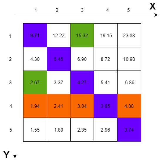
Figure 1. The similarity matrix between x and y. The elements marked green, orange and purple are sampled to illustrate the unsatisfied properties of the log-transformed Bayesian distance.

2.4. The New FCM Based on Generalized Likelihood Ratio

Generalized likelihood testing is defined as the ratio between the maximum value of the likelihood function with constraints to the maximum value of the likelihood function without constraints. The basic idea is that, if the parameters imposed on the model are valid, adding such a constraint should not lead to a significant decrease in the maximum value of the likelihood function. Considering Nakagami–Rayleigh distribution, for a pair of patches $(v_s\left(N_i\right),v_s\left(N_j\right))$ on a SAR image, we can define its likelihood ratio (LR)

$${\mathit{\psi }}_{LR}(v_s\left(N_i\right),v_s\left(N_j\right))=\frac{p(v_s\left(N_i\right),v_s\left(N_j\right),R_i=R_0,R_j=R_0;{\varkappa }_0)}{p(v_s\left(N_i\right),v_s\left(N_j\right),R_i=R_1,R_j=R_2;{\varkappa }_1)}$$

(22)

where ${\varkappa }_0$ and ${\varkappa }_1$ represent two hypotheses, defined as

$$\begin{array}{cc}\hfill {\varkappa }_0& :R_i=R_j=R_0\left(NullHypothesis\right)\hfill \\ \hfill {\varkappa }_1& :R_i=R_1;R_j=R_2;R_1\ne R_2\left(AlternativeHypothesis\right)\hfill \end{array}$$

(23)

$v_s\left(N_i\right)$ is the patch centered at pixel i, and $v_s\left(N_j\right)$ denotes the non-local patch centered at pixel j. $R_i$ and $R_j$ as the hypothesis parameters denote the noise-free backscatter value of center pixel i. Hypothesis ${\varkappa }_0$ means a parametric constraint on statistical distribution that the two patches $(v_s\left(N_i\right),v_s\left(N_j\right))$ come from the same distribution. Thus, they have the same backscatter value, formalized as $R_i=R_j=R_0$. Hypothesis ${\varkappa }_1$ means no constraint on the statistical distribution of $v_s\left(N_i\right)$ and $v_s\left(N_j\right)$, formalized as $R_i\ne R_j$. For the sake of mathematical simplicity, we choose parameters in this way

$$\begin{array}{cc}\hfill R_0& =\underset{\Theta }{max}p(v_s\left(N_i\right),v_s\left(N_j\right),R_i=R_j=R_0;{\varkappa }_0)\hfill \\ \hfill R_{1}or{R}_2& =\underset{R_1,R_2\in \Theta }{max}p(z_s\left(N_i\right),z_s\left(N_j\right),R_i=R_1,R_j=R_2;{\varkappa }_1)\hfill \end{array}$$

(24)

Thus, Equation (22) becomes the generalized likelihood ratio (GLR), defined as

$${\mathit{\psi }}_{GLR}(v_s\left(N_i\right),v_s\left(N_j\right))=\frac{{sup}_{R_0}p(v_s\left(N_i\right),v_s\left(N_j\right),R_i=R_j=R_0)}{{sup}_{R_1,R_2}p(v_s\left(N_i\right),v_s\left(N_j\right),R_i=R_1,R_j=R_2,R_1\ne R_2)}$$

(25)

where $0<{\psi }_{GLR}(v_s\left(N_i\right),v_s\left(N_j\right))<1$; the larger the ${\psi }_{GLR}(z_s\left(N_i\right),z_s\left(N_j\right))$, the larger the probability that hypothesis ${\varkappa }_{\mathbf{0}}$ holds, and the more inclined to accept ${\varkappa }_{\mathbf{0}}$. This also means that there is a higher probability of two patches $v_s\left(N_i\right)$ and $v_s\left(N_j\right)$ coming from the same distribution. Thus, we can use GLR to measure the similarity between two patches.

Unlike the Deledalle [37] approach, we construct the patch similarity as the continued product of corresponding pixel similarity. Next, we will give a detailed derivation.

Now, we assume $v_s\left(N_i\right)$ and $v_s\left(N_j\right)$ are irrelevant, and the corresponding pixel within the patch is independent. Thus, the similarity between $v_s\left(N_i\right)$ and $v_s\left(N_i\right)$ can be calculated by

$${\mathit{\psi }}_{\mathit{GLR}}({\mathit{v}}_{\mathit{s}}\left({\mathit{N}}_{\mathit{i}}\right),{\mathit{v}}_{\mathit{s}}\left({\mathit{N}}_{\mathit{j}}\right))=\prod _{k=1}^N{\mathit{\xi }}_{\mathit{GLR}}({\mathit{x}}_{\mathit{i}}^{\mathit{k}},{\mathit{x}}_{\mathit{j}}^{\mathit{k}})$$

(26)

where $N=s^2$ is the number of pixels in the patch, and ${\mathit{\xi }}_{\mathit{GLR}}({\mathit{x}}_{\mathit{i}}^{\mathit{k}},{\mathit{x}}_{\mathit{j}}^{\mathit{k}})$ is defined as

$$\begin{array}{cc}\hfill {\mathit{\xi }}_{\mathit{GLR}}({\mathit{x}}_{\mathit{i}}^{\mathit{k}},{\mathit{x}}_{\mathit{j}}^{\mathit{k}})& =\frac{{sup}_{R_0}p(x_i^k,x_j^k;R_1=R_2=R_0)}{{sup}_{R_1,R_2}p(x_i^k,x_j^k;R_i=R_1,R_j=R_2,R_1\ne R_2)}\hfill \\ \hfill & =\frac{{sup}_{R_0}\left[p(x_i^k,x_j^k;R_1=R_2=R_0)\right]}{\left[{sup}_{R_1}p(x_i^k;R_i=R_1)\right]\ast \left[{sup}_{R_2}p(x_j^k;R_j=R_2)\right]}\hfill \end{array}$$

(27)

$x_i^k$ and $x_j^k$ denote the kth pixel in patch; $R_0$, $R_1$, $R_2$ denote noise-free backscatter value. To obtain the maximum likelihood value ${sup}_{R_0}p(x_i^k,x_j^k,R_i=R_j=R_0)$, we need get joint probability

$$\begin{array}{cc}\hfill p(x_i^k,x_j^k;R_i=R_j=R_0)& =p(x_i^k;R_0)\ast p(x_j^k;R_0)\hfill \\ \hfill & ={\left(\frac{2}{\Gamma \left(L\right)}\right)}^2\ast {\left(\frac{L}{R_0}\right)}^{2L}\ast {\left(x_i^k{x}_j^k\right)}^{2L-1}\ast exp\left\{-\frac{L}{R_0}\left[{\left(x_i^k\right)}^2+{\left(x_j^k\right)}^2\right]\right\}\hfill \end{array}$$

(28)

To obtain the maximum likelihood estimator ${\widehat{R}}_0$ of $R_0$, we construct the maximum likelihood function

$$\begin{array}{cc}\hfill \mathcal{L}\left(R_0\right)& =\prod _{m=1}^{M}p(x_i^{k_m};R_0)\ast p(x_j^{k_m};R_0)\hfill \\ \hfill & =\prod _{m=1}^M{\left(\frac{2}{\Gamma \left(L\right)}\right)}^2\ast {\left(\frac{L}{R_0}\right)}^{2L}\ast {\left(x_i^{k_m}{x}_j^{k_m}\right)}^{2L-1}\hfill \\ \hfill & \ast exp\left\{-\frac{L}{R_0}\left[{\left(x_i^{k_m}\right)}^2+{\left(x_j^{k_m}\right)}^2\right]\right\}\hfill \end{array}$$

(29)

Then, making the logarithm on $\mathcal{L}\left(R_0\right)$ and differentiating

$$\begin{array}{cc}\hfill \frac{\partial ln\mathcal{L}\left(R_0\right)}{\partial R_0}=\frac{\partial }{\partial R_0}\{& \sum _{m=1}^{M}ln\frac{4L^{2L}}{{\Gamma }^2\left(L\right)}-2Lln{R}_0+(2L-1)ln\left(x_i^{k_m}{z}_j^{k_m}\right)-\frac{L}{R_0}\left[{\left(x_i^{k_m}\right)}^2+{\left(x_j^{k_m}\right)}^2\right]\}\hfill \\ \hfill & =-\frac{2LM}{R_0}+\frac{L}{R_0^2}\sum _{m=1}^M\left[{\left(x_i^{k_m}\right)}^2+{\left(x_j^{k_m}\right)}^2\right]\hfill \end{array}$$

(30)

Let $\frac{\partial ln\mathcal{L}\left(R_0\right)}{\partial R_0}=0$; then, we get

$${\widehat{R}}_0=\frac{1}{2M}\sum _{m=1}^M\left[{\left(x_i^{k_m}\right)}^2+{\left(x_j^{k_m}\right)}^2\right]$$

(31)

considering that there is only one available observation for each pixel in the patch, that is to say $M=1$; thus, we can get

$${\widehat{R}}_0=\frac{1}{2}\left[{\left(x_i^k\right)}^2+{\left(x_j^k\right)}^2\right]$$

(32)

With the same derivation process as above, we can obtain the maximum likelihood estimator ${\widehat{R}}_1$ and ${\widehat{R}}_2$ for $R_1$ and $R_2$

$$\begin{array}{c}\hfill {\widehat{R}}_1={\left(x_i^k\right)}^2\\ \hfill {\widehat{R}}_2={\left(x_j^k\right)}^2\end{array}$$

(33)

Now, we replace $R_0$, $R_1$, $R_2$ with maximum likelihood estimators ${\widehat{R}}_0$, ${\widehat{R}}_1$, and ${\widehat{R}}_2$ in Equation (27); then, we get the similarity between corresponding pixels

$$\begin{array}{cc}\hfill & {\xi }_{\mathit{GLR}}({\mathit{x}}_{\mathit{i}}^{\mathit{k}},{\mathit{x}}_{\mathit{j}}^{\mathit{k}})=\frac{{sup}_{R_0}p(x_i^k,x_j^k;R_1=R_2=R_0)}{{sup}_{R_1,R_2}p(x_i^k,x_j^k;R_i=R_1,R_j=R_2,R_1\ne R_2)}\hfill \\ \hfill & =\frac{\frac{4L^{2L}}{\Gamma \left(L\right)}\ast {\left\{\frac{1}{2}\left[{\left(x_i^k\right)}^2+{\left(x_j^k\right)}^2\right]\right\}}^{-2L}\ast {\left(x_i^k{x}_j^k\right)}^{2L-1}\ast exp(-2L)}{\left\{\frac{2L^L}{\Gamma \left(L\right)}{\left(x_i^k\right)}^{-2L}\ast {\left(x_i^k\right)}^{2L-1}\ast exp(-L)\right\}\ast \left\{\frac{2L^L}{\Gamma \left(L\right)}{\left(x_j^k\right)}^{-2L}\ast {\left(x_j^k\right)}^{2L-1}\ast exp(-L)\right\}}\hfill \end{array}$$

(34)

After simplifying Equation (34), we get

$${\xi }_{\mathit{GLR}}({\mathit{x}}_{\mathit{i}}^{\mathit{k}},{\mathit{x}}_{\mathit{j}}^{\mathit{k}})={\left[\frac{2x_i^k{x}_j^k}{{\left(x_i^k\right)}^2+{\left(x_j^k\right)}^2}\right]}^{2L}$$

(35)

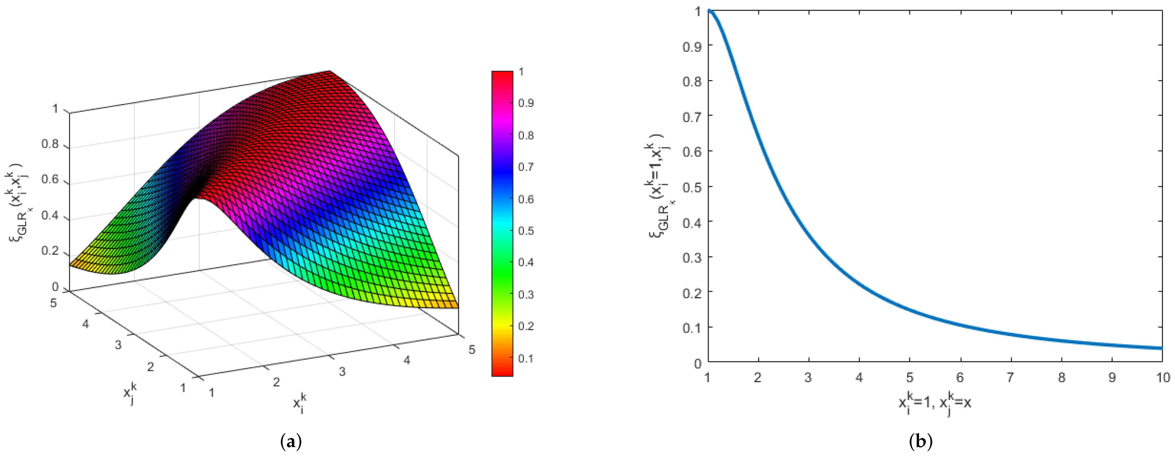
Equation (35) can measure the similarity between corresponding pixels within two patches. Figure 2a shows the similarity ${\xi }_{GLR}(x_i^k,x_j^k)$, where $x_i^k=[1,2,3,4,5]$ and $x_j^k=[1,2,3,4,5]$. From Figure 2a we can see that the Properties 1 and 3 mentioned earlier can be satisfied. Figure 2b is the change curve of similarity ${\xi }_{GLR}(x_i^k,x_j^k)$ when $x_i^k$ is fixed at 1 and $x_j^k=[1,2,\dots ,10]$. The maximum ${\xi }_{GLR}(x_i^k,x_j^k)$ can be obtained when $x_i^k=x_j^k=1$. Besides, ${\xi }_{GLR}(x_i^k,x_j^k)$ gradually decreases with increasing distance. Thus, Property 2 can be proved.

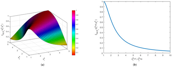
Figure 2. The similarity value ${\xi }_{GLR}(x_i^k,x_j^k)$ based on GLR. (a) The X and Y axes indicate values of $x_i^k$ and $x_j^k$. (b) The similarity when $x_i^k=1$ and $x_j^k$ are taken from 1 to 10.

Therefore, by putting Equation (35) into Equation (26), a patch similarity metric based on GLR can be derived as follows

$${\mathit{\psi }}_{\mathit{GLR}}({\mathit{v}}_{\mathit{s}}\left({\mathit{N}}_{\mathit{i}}\right),{\mathit{v}}_{\mathit{s}}\left({\mathit{N}}_{\mathit{j}}\right))=\prod _{k=1}^N{\xi }_{\mathit{GLR}}({\mathit{x}}_{\mathit{i}}^{\mathit{k}},{\mathit{x}}_{\mathit{j}}^{\mathit{k}})=\prod _{k=1}^N\left[\frac{2z_i^k{x}_j^k}{{\left(x_i^k\right)}^2+{\left(x_j^k\right)}^2}\right]$$

(36)

We then can use this similarity metric based on GLR (Equation (36)) to obtain the weight of each patch in a non-local search space centered at pixel i. Then the recovered amplitude of pixel i in in SAR image can be calculated as follows

$${\tilde{x}}_i=\sum _{j\in W_i^r}{\mathit{\psi }}_{\mathit{GLR}}({\mathit{v}}_{\mathit{s}}\left({\mathit{N}}_{\mathit{i}}\right),{\mathit{v}}_{\mathit{s}}\left({\mathit{N}}_{\mathit{j}}\right))\ast {\mathit{x}}_{\mathit{j}}$$

(37)

where ${\tilde{x}}_i$ is the estimator of the ith pixel, ${\mathit{\psi }}_{\mathit{GLR}}({\mathit{v}}_{\mathit{s}}\left({\mathit{N}}_{\mathit{i}}\right),{\mathit{v}}_{\mathit{s}}\left({\mathit{N}}_{\mathit{j}}\right))$ is the weight between patch $v_s\left(N_i\right)$ and $v_s\left(N_j\right)$. After visiting all pixels in SAR image, we can construct an auxiliary image $\tilde{I}=\left\{{\tilde{x}}_1,{\tilde{x}}_2,\dots {\tilde{x}}_i,\dots ,{\tilde{x}}_N\right\}$. Then $\tilde{I}$ is added into the objective function of standard FCM as non-local spatial information term and we can obtain GLR_FCM

$$\begin{array}{cc}\hfill min{J}_m& (U,V)=\sum _{k=1}^c\sum _{i=1}^N{u}_{ki}^m\left||x_i-v_k\right|{|}^2+\sum _{k=1}^c\sum _{i=1}^N{\eta }_i{u}_{ki}^m\left||{\tilde{x}}_i-v_k\right|{|}^2\hfill \\ \hfill & s.t.\sum _{k=1}^c{u}_{ki}=1,0\le u_{ki}\le 1,0\le \sum _{i=1}^N{u}_{ki}\le N\hfill \end{array}$$

(38)

By minimizing Equation (38) using Lagrange multiplier method, the membership degree $u_{ki}$ and cluster $v_k$ can be updated by

$$u_{ki}=\frac{1}{{\sum }_{j=1}^c{\left(\frac{{∥x_i-v_k∥}^2+{\eta }_i{∥\widetilde{x_i}-v_k∥}^2}{{∥x_i-v_j∥}^2+{\eta }_i{∥\widetilde{x_i}-v_j∥}^2}\right)}^{\frac{1}{m-1}}}$$

(39)

$$v_k=\frac{{\sum }_{i=1}^N\left(u_{ki}^m{x}_i+{\eta }_i{u}_{ki}^m\widetilde{x_i}\right)}{{\sum }_{i=1}^N\left(u_{ki}^m+{\eta }_i{u}_{ki}^m\right)}$$

(40)

In the objective function of LBNL_FCM and GLR_FCM, an adaptive factor based on local intensity entropy ${\eta }_i$ is introduced to balance the original detail information and non-local spatial information. ${\eta }_i$ is defined as

$$\begin{array}{cc}\hfill & {\eta }_i=\alpha \times \frac{exp(max{E}_i)-exp\left(E_i\right)}{exp(max{E}_i)-1}\hfill \\ \hfill & \alpha =Med\left\{{\sigma }_1,{\sigma }_2,\dots ,{\sigma }_i,\dots ,{\sigma }_{N-1},{\sigma }_N\right\}\hfill \end{array}$$

(41)

where $E_i=-{\sum }_{j=1}^k{p}_{i}log\left(p_i\right)$ denotes the information entropy of the local area histogram at the ith pixel. k is the number of quantized gray levels. ${\sigma }_i$ denotes the local variance at the ith pixel, $Med$ indicates a median operation, and N is the total number of pixels.

In Equation (41), ${\eta }_i$ is determined by the local intensity entropy $E_i$. In the homogeneous region, the amplitude values tend to be the same, and $E_i$ is small; hence, a large weight ${\eta }_i$ will be assigned for non-local spatial information. Conversely, at the edges, where the local entropy $E_i$ is relatively large, and ${\eta }_i$ receives a small value, the original SAR information is given more consideration.

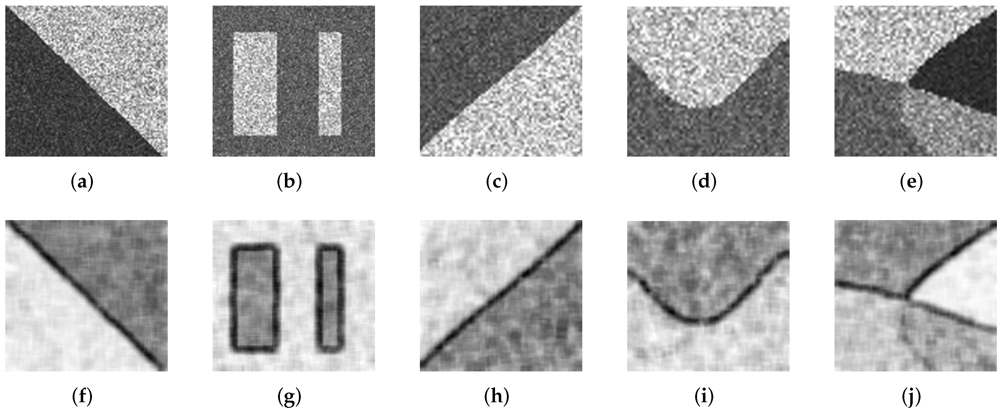
Figure 3a–e are original SAR image slices and Figure 3f–j are the ${\eta }_i$ maps for Figure 3a,b, respectively. We can see a black color near the edge, which indicates that the intensity value of ${\eta }_i$ at the edge is small and relatively large in the homogeneous regions. Thus, the original image information and non-local spatial information can be dynamically balanced and adjusted.

Figure 3. The results of dynamically balanced factor ${\eta }_i$. (a–e) Five sample SAR image slices. (f–j) ${\eta }_i$ maps of (a–e), respectively.

2.5. The Membership Degree Smoothing and Label Correction

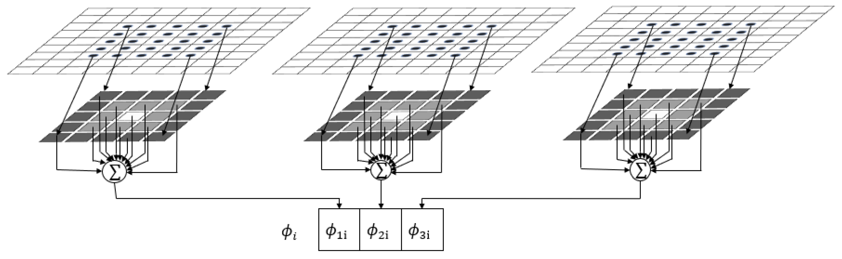
In addition to non-local spatial information, local spatial information is also useful. For a pixel, its class should be influenced by the surrounding pixels. Thus, we add membership degree smoothing into the iteration process. For the ith pixel in the SAR image, we sum the membership vector of the neighborhood pixels to obtain a weight vector ${\varphi }_i({\varphi }_i= \left[{\varphi }_{1i}{\varphi }_{2i}\dots {\varphi }_{ci}\right])$, and ${\varphi }_i$ is weighted to the membership vector of the ith pixel. Then we can get the new membership degree $u_i^{\prime }$ for the ith pixel.

$$\begin{array}{c}\hfill {\varphi }_{ki}=\sum _{j\in N_i}{u}_{kj}\\ \hfill u_i^{{}^{\prime }}=u_i•{\varphi }_i\end{array}$$

(42)

where $N_i$ is the neighborhood pixels of the ith pixel, $u_i$ is the membership before smoothing, and $u_i^{\prime }$ is the weighted membership degree. Figure 4 shows the calculation process.

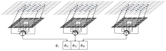
Figure 4. The calculation process of weight vector ${\varphi }_i$ for three classes. In this example, the neighborhood size is specified as $5\times 5$.

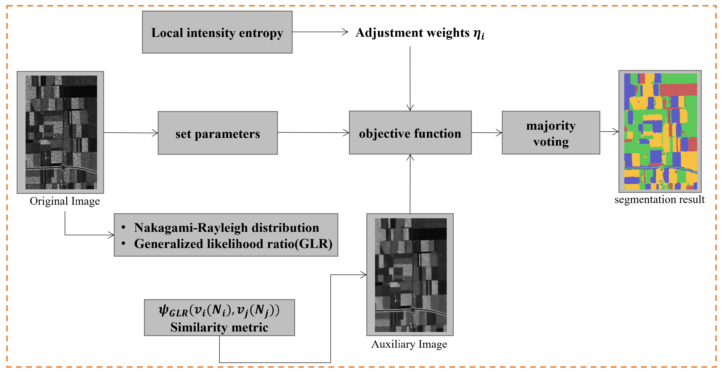
Besides, label correction is used as a homogeneous region smoothing technique in SAR segmentation in [42]. It has been shown to be effective in the correction of error class labels. Hence, we will adopt a simple method to correct the error pixel class. This framework uses the majority voting strategy to revise the error pixel label upon completion of the iteration. Specifically, a fixed-scale window is utilized to slide over the image. The class label with the largest number in the slid window is the final class of the central pixel. Figure 5 shows that the framework of GLR_FCM and LBNL_FCM is alike.

Figure 5. The framework of proposed segmentation algorithm GLR_FCM, and the LBNL_FCM is similar.

3. Experiments and Results

In this section, we perform LBNL_FCM and GLR_FCM on simulated SAR images and real SAR images to illustrate the effectiveness of our proposed algorithms. The segmentation results are evaluated qualitatively and quantitatively. Several popular improved FCM algorithms are used as baselines to illustrate the advantages of the proposed algorithms in edge preservation and region consistency. These methods are FCM [22], FCM_S1 and FCM_S2 [24], KFCM_S1 and KFCM_S2 [24], EnFCM [25], FGFCM [26], FCM_NLS [31], NS_FCM [34], and RFCM_BNL [35]. Note that, for real SAR images, we focus more on visual inspection because it is difficult to obtain its ground truth. Experiment images are selected from four different satellites, including AIRSAR, ALOS PolSAR, TerraSAR-X, and GF3.

3.1. Experimental Setting

For all algorithms, the parameters are selected as follows: The stopping threshold $\delta ={10}^{-5}$, Maximum iterations $T=200$, membership exponent $m=2$. We set $\alpha =5$ for FCM_S1, FCM_S2, KFCM_S1, KFCM_S2, EnFCM, and FCM_NLS. According to [34], we set $\alpha =6$ for NS_FCM. ${\lambda }_s$ and ${\lambda }_g$ in FGFCM are set to 2 and 7, respectively. For NS_FCM and FCM_NLS, the local neighbor size is $5\times 5$, and the non-local search window is set to $11\times 11$ and $15\times 15$, respectively. For RFCM_BNL, LBNL_FCM and GLR_FCM, the local neighbor window is set to $3\times 3$ and the non-local search window is set to $15\times 15$, $9\times 9$, and $23\times 23$. For LBNL_FCM and GLR_FCM, the membership degree smoothing and label correction window is set to $5\times 5$. In LBNL_FCM and GLR_FCM, when calculating ${\eta }_i$, the gray level is quantized into 16 bins, i.e., $k=16$.

3.2. Evaluation Indicators

Evaluating results is a key step in measuring the effectiveness of the algorithms. In this paper, the effectiveness of the proposed and reference algorithms is assessed from both objective and subjective aspects. Moreover, we concentrate on two crucial aspects of the segmentation results: Compactness and separation. Whether it is a visual inspection by human eyes or a quantitative evaluation, a good segmentation algorithm should make the intra-class dissimilarity as small as possible and the inter-class variability as large as possible, i.e., corresponding to compactness and separation, respectively. Table 1 shows several assessment indicators that we intend to use to quantitatively evaluate these two properties, whose efficacy was proved in [43].

Table 1. The quantitative evaluation indicators used in simulation SAR image experiments for results.

Indicator	Formulation	Description
PC (Partition Coefficient) [44]	$PC=\frac{1}{N}{\sum }_{c=1}^c{\sum }_{i=1}^N{u}_{ci}^2$	The larger the PC value, the better the partition result
PE (Partition Entropy) [45]	$PE=-\frac{1}{N}{\sum }_{c=1}^c{\sum }_{i=1}^N{u}_{ci}log\left(u_{ci}\right)$	The smaller the PE value, the better the partition result
MPC (Modified PC) [46]	$\begin{array}{c}MPC=\frac{C\times PC-1}{C-1}\\ PC=\frac{1}{N}{\sum }_{c=1}^c{\sum }_{i=1}^N{u}_{ci}^2\end{array}$	The MPC eliminates the dependency on c, the large the MPC is, the better the partition result
MPE (Modified PE) [46]	$\begin{array}{c}MPE=\frac{N\times PE}{N-C}\\ PE=-\frac{1}{N}{\sum }_{c=1}^c{\sum }_{i=1}^N{u}_{ci}log\left(u_{ci}\right)\end{array}$	Similar to above that the smaller the MPE is, the better the partition result
FS (Fukuyama-Sugeno Index) [47]	$\begin{array}{c}FS=J_m(U,V)-K_m(U,V)\\ =J_m-{\sum }_{i=1}^N{\sum }_{c=1}^c{u}_{ci}^m{∥v_c-\tilde{v}∥}^2\\ \mathrm{where}\tilde{v}=\frac{1}{N}{\sum }_{i=1}^N{x}_i\end{array}$	The first term indicates the compactness and the second term indicates the separation. And the minimum FS implies the optimal partition

3.3. Segmentation Results on Simulated SAR Images

We can obtain accurate ground truth for simulated SAR images, so we use segmentation accuracy to evaluate the segmentation performance. In addition, five numerical evaluation indexes are computed. The segmentation accuracy is defined as the number of correctly segmented pixels divided by the total number of pixels, and the formula is as follows:

$$SA=\frac{{\sum }_{k=1}^c{A}_k\bigcap C_k}{{\sum }_{j=1}^c{C}_j}$$

(43)

where c represents the number of segmentation objects, $C_k$ denotes the number of pixels within the kth class in the real SAR image, $A_k$ indicates the number of pixels belonging to the kth class in the segmentation result, and ${\sum }_{j=1}^c{C}_j$ corresponds to the total number of pixels.

3.3.1. Experiment 1: Testing on the First Simulated SAR Image

The first experiments are carried out on a one-look simulated SAR image with 250 × 200 pixels as shown in Figure 6a. This simulated SAR image includes five classes with intensity value taken as 10, 50, 100, 150, 200. Its gray and color ground truth are shown in Figure 6b,c.

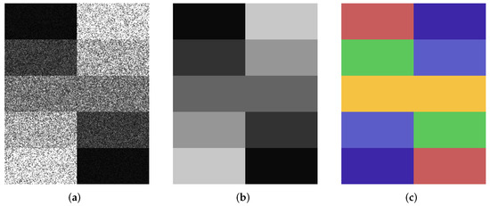
Figure 6. The simulated SAR image and ground truth. (a) Simulated SAR image; (b) ground truth with gray; (c) ground truth with color.

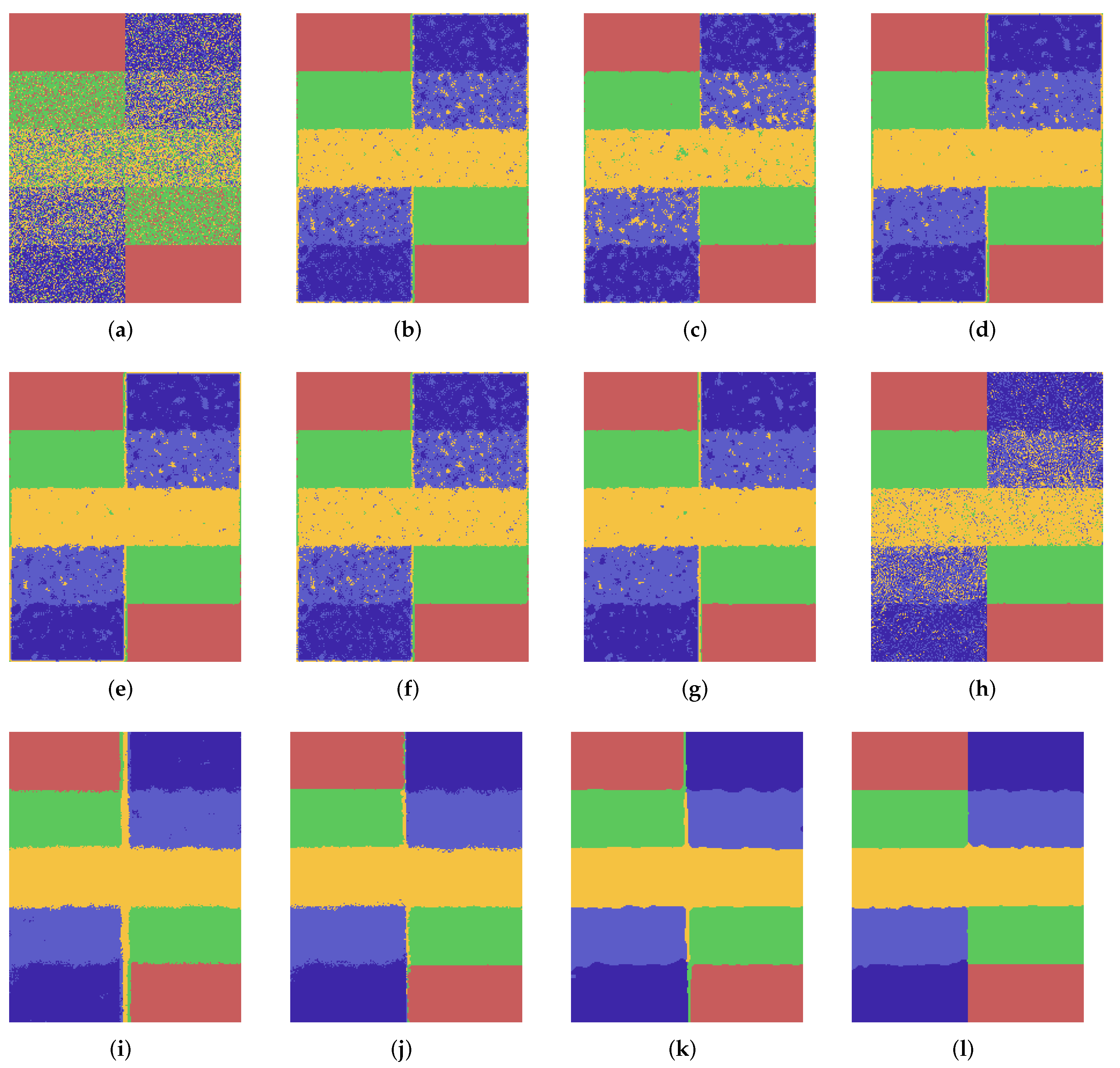
The experiment results of the proposed algorithms and comparative algorithms are shown in Figure 7. It can be seen that the original FCM has the worst result in regional consistency and many noise points are present. FCM_S1 and FCM_S2 enhance the segmentation result by adding local information. The kernel distance versions of KFCM_S1 and KFCM_S2 obtain further enhancement results. Nevertheless, there are still plenty of noise pixels. The reason is that the local neighborhood information on SAR images is contaminated by noise. The reliability of local spatial information is severely weakened, which ultimately leads to the failure of segmentation.

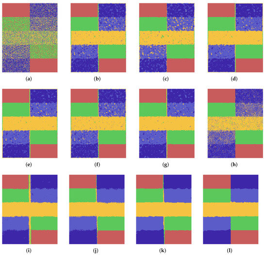
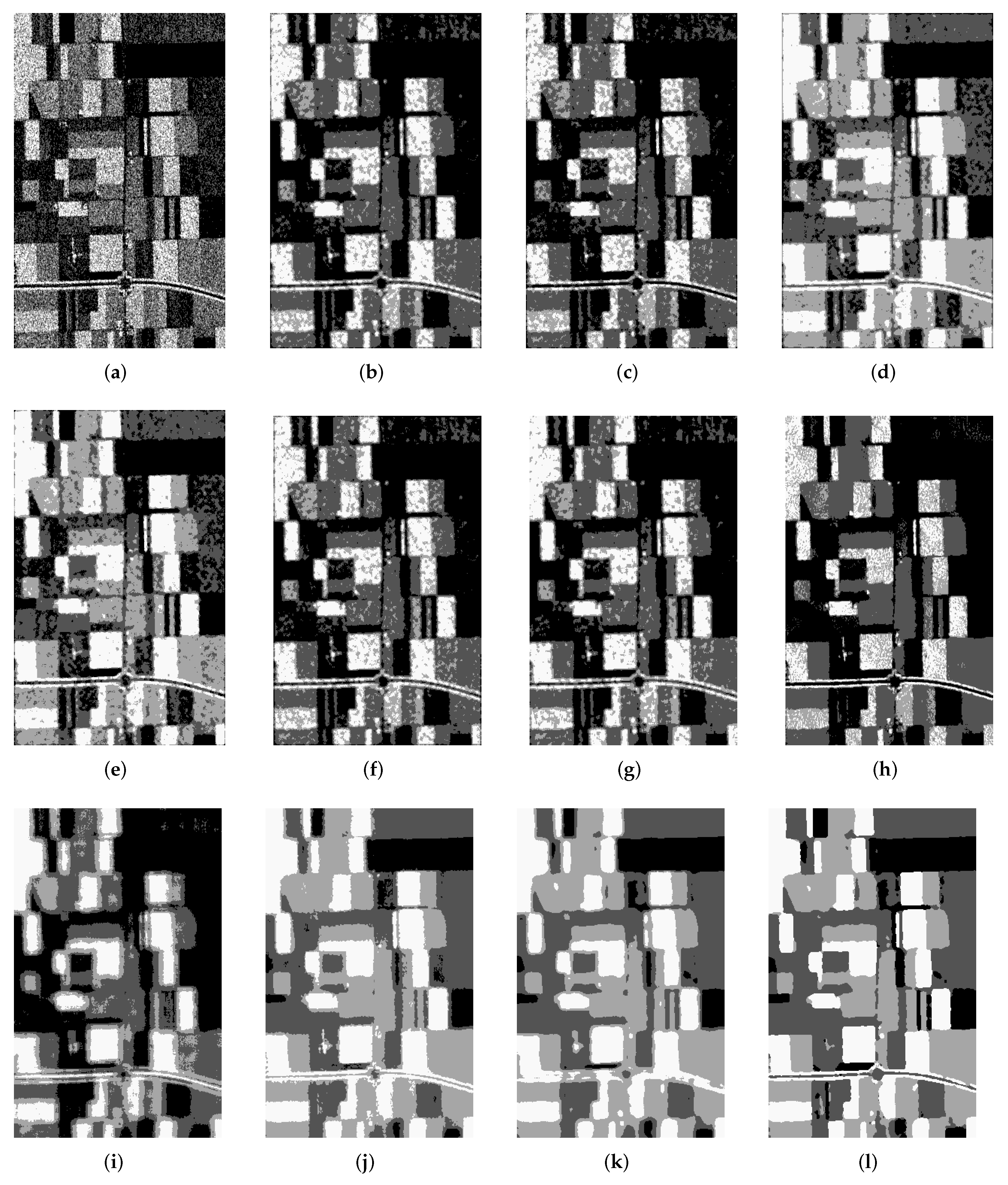
Figure 7. The segmentation results on simulated SAR image. (a) FCM. (b) FCM_S1. (c) FCM_S2. (d) KFCM_S1. (e) KFCM_S2. (f) EnFCM. (g) FGFCM. (h) FCM_NLS. (i) NS_FCM. (j) RFCM_BNL. (k) LBNL_FCM. (l) GLR_FCM.

FCM_NLS and NS_FCM in Figure 7h,i consider the non-local information. However, the non-local spatial information is measured by Euclidean distance, which is inappropriate for SAR images. So they still have significant misclassification problems. The RFCM_BNL takes into account the characteristics of SAR images and therefore achieves a relatively good result in terms of the regional coherence. However, there is still a large number of isolated pixels near the edges. The result of LBNL_FCM presents a better continuity of edges and homogeneous regions cleaner than that of RFCM_BNL. However, the Bayesian-based FCM algorithm is not the best in terms of edge preservation in Figure 7j,k. There is a serious misclassification phenomenon at the edges, i.e., the region between the green region and the blue region is divided into yellow class. In Figure 7l, GLR_FCM achieves the best visual result for maintaining regional consistency and edge preservation. Effectively eliminating the false class of RFCM_BNL and LBNL_FCM at the edges and almost no isolated noise pixels.

Table 2 displays the SA (%) and executed time of each algorithm. We see that the kernel method is valid for results. The non-local information is more useful for SAR image segmentation compared to local information. Because of the statistical property of SAR images, higher segmentation accuracy is obtained by FCM_RBNL, LBNL_FCM and GLR_FCM. Besides, GLR_FCM obtains the best segmentation accuracy of 99.16%, consistent with the visualization in Figure 7. The algorithms based on the non-local information have higher time consumption because each pixel is visited in computing auxiliary.

Table 2. SA (%) and executed time(s) on the first simulated SAR image.

Method	SA (%)	Time (s)	Method	SA (%)	Time (s)
FCM	60.58	2.16	FGFCM	94.65	5.64
FCM_S1	90.49	1.11	FCM_NLS	83.61	7.27
FCM_S2	90.49	1.46	NS_FCM	95.03	7.77
KFCM_S1	92.66	1.27	RFCM_BNL	97.29	10.88
KFCM_S2	91.42	1.20	LBNL_FCM	97.64	12.11
EnFCM	90.63	1.85	GLR_FCM	99.16	17.73

Table 3 shows the quantitative evaluation for the first simulated SAR image. $V_{PC}$ and $V_{MPC}$ express the fuzziness of the partition result. The larger the value, the better the partition result. In contrast, the minimums of $V_{PE}$ and $V_{MPE}$ imply the optimal result. The $V_{FS}$ describes the compactness and separation. The best partition can be obtained with the minimum $V_{FS}$. In addition to the optimal value obtained by the NS_FCM on $V_{FS}$, the LBNL_FCM and GLR_FCM obtain the best value in the other criteria.

Table 3. Quantitative evaluation on the first simulated SAR image.

Method	${\mathit{V}}_{\mathit{PC}}$	${\mathit{V}}_{\mathit{PE}}$	${\mathit{V}}_{\mathit{MPC}}$	${\mathit{V}}_{\mathit{MPE}}$	${\mathit{V}}_{\mathit{FS}}$
FCM	0.7994	0.3995	0.7492	0.3995	$-3.12\times {10}^8$
FCM_S1	0.7203	0.5581	0.6504	0.5582	$-1.36\times {10}^8$
FCM_S2	0.7350	0.5347	0.6688	0.5347	$-1.78\times {10}^8$
KFCM_S1	0.6783	0.6623	0.5978	0.6624	$-1.01\times {10}^8$
KFCM_S2	0.6861	0.6537	0.6076	0.6537	$-1.39\times {10}^8$
EnFCM	0.8518	0.3031	0.8147	0.3031	$-1.56\times {10}^8$
FGFCM	0.8750	0.2595	0.8438	0.2595	$-2.33\times {10}^8$
FCM_NLS	0.7175	0.5892	0.6469	0.5893	$-1.70\times {10}^8$
NS_FCM	0.6932	0.6342	0.6165	0.6342	$-9.03\times {10}^7$
RFCM_BNL	0.8069	0.4165	0.7587	0.4165	$-1.34\times {10}^8$
LBNL_FCM	0.9609	0.0792	0.9511	0.0792	$-1.54\times {10}^8$
GLR_FCM	0.9855	0.0260	0.9819	0.0260	$-1.78\times {10}^8$

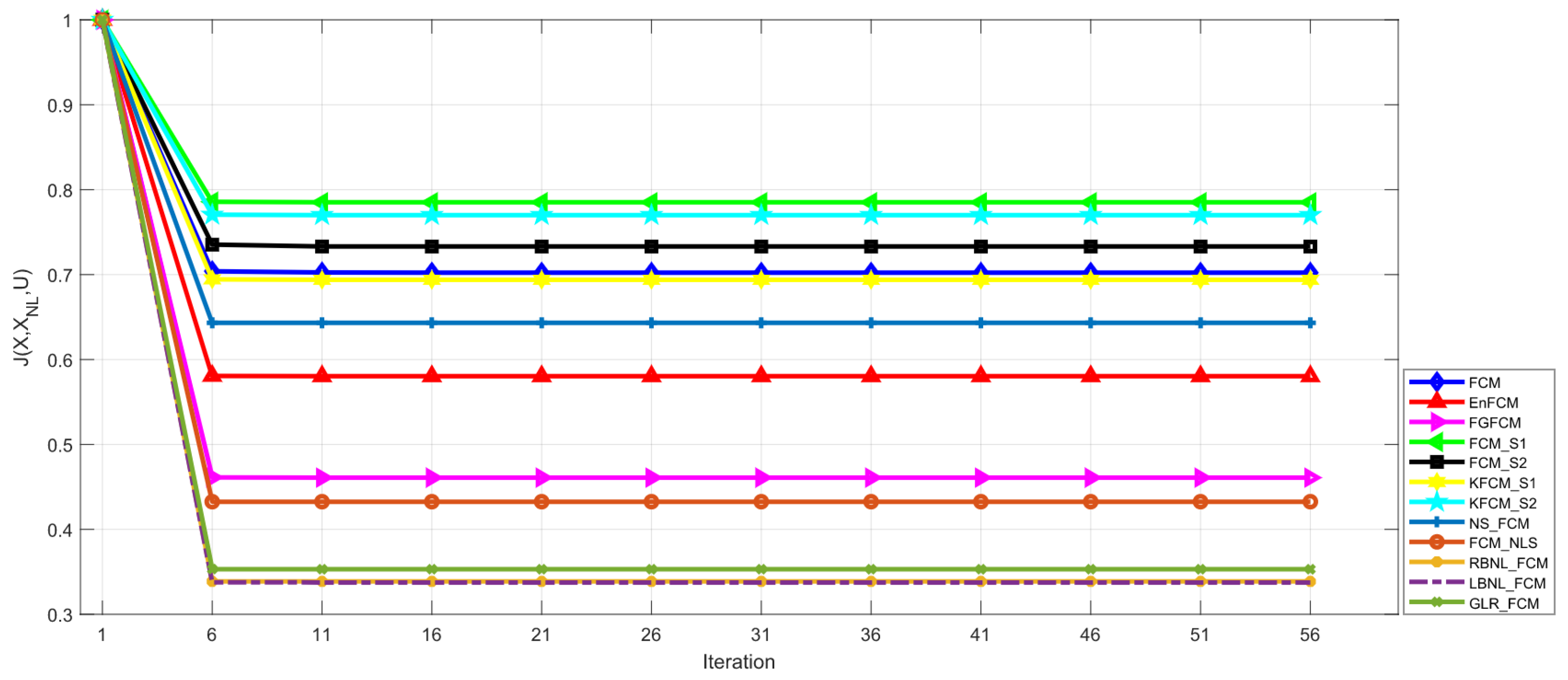
Figure 8 provides the change curve of the objective function. We can see that the objective function of LBNL_FCM descends fastest and obtains the minimum value. The objective function of GLR_FCM decreases at a similar speed to that of LBNL_FCM. Moreover, a relatively small value of the objective function is obtained.

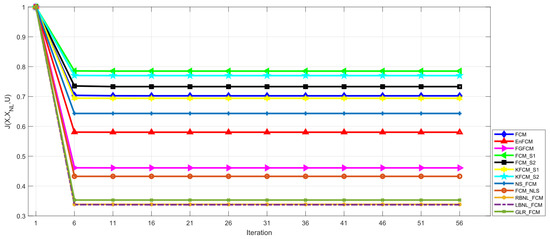
Figure 8. The objective function change curve of each algorithm on the first simulated SAR image.

3.3.2. Experiment 2: Testing on the Second Simulated SAR Image

The second simulated SAR image is composed of 283 × 283 pixels, and includes five classes with amplitude values settled as (0, 64, 128, 192, 255). Figure 9a–c show the original simulated SAR image and the ground truth. Figure 9d–o show the segmentation results of each algorithm.

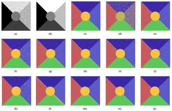
Figure 9. The segmentation results on the second simulated SAR image. (a) Original Image (b) Ground Truth (Gray) (c) Ground Truth (Color) (d) FCM (e) FCM_S1 (f) FCM_S2 (g) KFCM_S1 (h) KFCM_S2 (i) EnFCM (j) FGFCM (k) FCM_NLS (l) NS_FCM (m) RFCM_BNL (n) LBNL_FCM (o) GLR_FCM.

Visually, the result of FCM (Figure 9d) has plenty of noise points. In Figure 9e–j, due to integration of the local spatial information, the isolated speckle pixels are significantly suppressed. The result of FCM_NLS obtains a better region consistency in red and green classes. However, there are still some blocks that are not properly classified under other categories. The results of NS_FCM and RFCM_BNL yield good regional coherence and smoothed edges. However, there are still serious classification mistakes on the periphery of different regions. In contrast, LBNL_FCM and GLR_FCM obtain relatively satisfactory segmentation results. Isolated pixels and blocks of speckle noise are practically non-existent there in homogeneous regions. In terms of structural information, GLR_FCM protects the continuity and smoothness of the edges, even when crossing regions with similar magnitude values. The edge can be well discriminated as shown in Figure 9o. Only slightly blurred edges exist at the nodes adjacent to the three regions.

A conclusion similar to the first experiment can be obtained from Table 4. In SAR image, non-local spatial information is more robust to speckle noise compared to local information. Thus, the FCMs with the non-local information terms obtain relatively good segmentation accuracy above 96%. However, they are time consuming because of the auxiliary image calculated in advance.

Table 4. SA (%) and executed time(s) on the second simulated SAR image.

Method	SA (%)	Time (s)	Method	SA (%)	Time (s)
FCM	73.82	3.47	FGFCM	97.88	9.36
FCM_S1	95.83	1.16	FCM_NLS	95.03	8.85
FCM_S2	96.55	1.27	NS_FCM	96.10	9.59
KFCM_S1	96.36	1.02	RFCM_BNL	98.66	16.58
KFCM_S2	96.94	1.22	LBNL_FCM	98.82	16.83
EnFCM	95.88	2.03	GLR_FCM	99.86	18.45

The quantitative evaluation indicators of each algorithm are recorded in Table 5. GLR_FCM obtains the optimal value on $V_{PC}$, $V_{PE}$, $V_{MPC}$, and $V_{MPE}$ and significantly outperforms other algorithms. The LBNL_FCM has relatively optimal indicators. On $V_{FS}$, EnFCM obtains the minimum value of $-6.27\times {10}^9$.

Table 5. Quantitative evaluation of the second simulated SAR image.

Method	${\mathit{V}}_{\mathit{PC}}$	${\mathit{V}}_{\mathit{PE}}$	${\mathit{V}}_{\mathit{MPC}}$	${\mathit{V}}_{\mathit{MPE}}$	${\mathit{V}}_{\mathit{FS}}$
FCM	0.8354	0.3298	0.7943	0.3298	$-6.28\times {10}^8$
FCM_S1	0.8204	0.3667	0.7755	0.3667	$-4.76\times {10}^8$
FCM_S2	0.8298	0.3524	0.7872	0.3524	$-5.34\times {10}^8$
KFCM_S1	0.7880	0.4492	0.7351	0.4492	$-4.34\times {10}^8$
KFCM_S2	0.7923	0.4448	0.7404	0.4448	$-4.86\times {10}^8$
EnFCM	0.9060	0.1971	0.8825	0.1971	$-6.27\times {10}^9$
FGFCM	0.9307	0.1511	0.9134	0.1511	$-5.66\times {10}^8$
FCM_NLS	0.8171	0.3890	0.7714	0.3890	$-4.90\times {10}^8$
NS_FCM	0.8085	0.4102	0.7607	0.4103	$-4.26\times {10}^8$
RFCM_BNL	0.8939	0.2414	0.8674	0.2414	$-4.79\times {10}^8$
LBNL_FCM	0.9882	0.0208	0.9852	0.0208	$-4.99\times {10}^8$
GLR_FCM	0.9972	0.0051	0.9965	0.0051	$-5.24\times {10}^8$

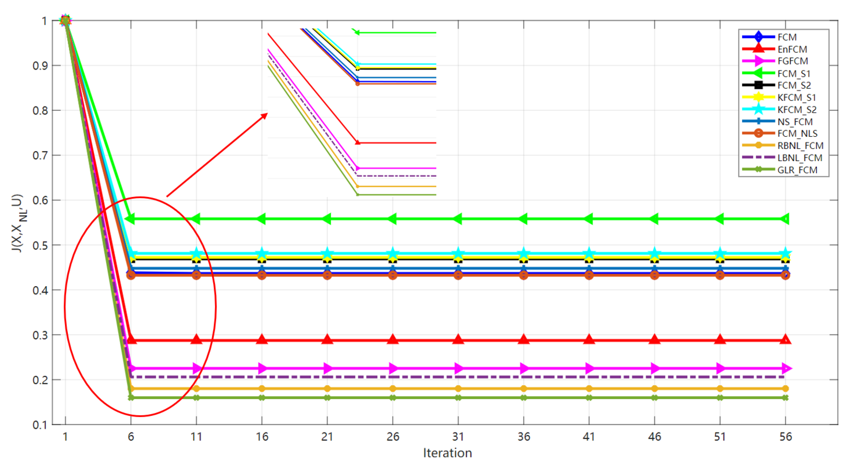
Figure 10 shows the curve of objective function on the second simulated SAR image. It can be seen that FCM_RBNL, LBNL_FCM, and GLR_FCM consider the statistical properties of SAR images, so their objective function decreases fastest and only needs two iterations to converge. In addition, at the convergence, GLR_FCM has the minimum loss value of the objective function. This also implies best segmentation performance.

Figure 10. The objective function curve of each algorithm on the second simulated SAR image.

3.4. Segmentation Results on Real SAR Images

Experiments on simulated SAR images only illustrate the validity and feasibility of algorithms. Therefore, we will test the practicality of proposed algorithms on real SAR images taken from different satellites. It is difficult to get ground truths for real SAR images; thus, segmentation results are accessed mainly by visual inspection.

3.4.1. Experiment 1: Experiment on the First Real SAR Image

The first experiment was carried out on an L-band, HH-polarized, SAR image with 2 m spatial resolution taken by AIRSAR in the Flevoland area of the Netherlands, as shown in Figure 11a. This area includes roughly four crop types, and the amplitudes are bright, dark, darker, and black. Figure 12 shows the segmentation results.

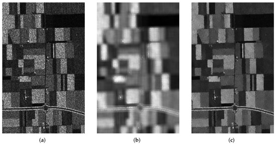
Figure 11. The first real SAR image and auxiliary images. (a) Original real SAR image; (b) The auxiliary image of LBNL_FCM; (c) The auxiliary image of GLR_FCM.

Figure 12. The segmentation result of each algorithm on the real SAR image. (a) FCM. (b) FCM_S1. (c) FCM_S2. (d) KFCM_S1. (e) KFCM_S2. (f) EnFCM. (g) FGFCM. (h) FCM_NLS. (i) NS_FCM. (j) RFCM_BNL. (k) LBNL_FCM. (l) GLR_FCM.

The auxiliary images of LBNL_FCM and GLR_FCM are shown in Figure 11b,c. The auxiliary image used by LBNL_FCM (see Figure 11b) strongly suppresses the noise and has a strong smoothing ability. The auxiliary image used in GLR_FCM (see Figure 11c reduces speckle noise while retaining the structural information. However, a slight texture noise remains inside the homogeneous region, which can be easily attenuated or removed by local information such as membership smoothing.

The most terrible result is provided by FCM in Figure 12a and almost fails when processing SAR images. The FCM_S1, FCM_S2, and the kernel methods suppress the noise to some extent. However, the results are still not very desirable. The EnFCM and FGFCM enhance the consistency of segmented regions compared with the previous methods by incorporating local information and using the histogram as the segmentation object. However, the darker region is misclassified to dark class from Figure 12f,g. FCM_NS has a better region coherence than FCM_NLS, but there is still severe misclassification in the region with similar intensity. Among these methods, RFCM_BNL, LBNL_FCM, and GLR_FCM obtain relatively satisfactory results. Visually, the segmentation results almost correctly reflect the region information of the original image. The large regions which are misclassed in other algorithms are correctly classified. However, the edges in RFCM_BNL and LBNL_FCM are not satisfactory enough, as shown in Figure 12j,k. A third class may appear in the middle of two adjacent regions. The result of GLR_FCM effectively overcomes this problem with the suitable similarity properties. Besides, most of the structure information is preserved in Figure 12l. A balance between regional homogeneity and edge preservation can be achieved well.

3.4.2. Experiment 2: Experiment on the Second Real SAR Image

An L-band, HH-polarized SAR image taken by AIRSAR is selected in this experiment. Figure 13a presents the original image. This area contains four kinds of crops shown as bright, gray, dark, and black. Figure 13a shows that the region with the brightest magnitude suffers from speckle noise. There is a gradual change in amplitude value.

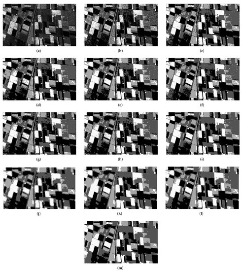
Figure 13. The segmentation results of each algorithms on the real SAR image. (a) Original image. (b) FCM. (c) FCM_S1. (d) FCM_S2. (e) KFCM_S1. (f) KFCM_S2. (g) EnFCM. (h) FGFCM. (i) FCM_NLS. (j) NS_FCM. (k) RFCM_BNL. (l) LBNL_FCM. (m) GLR_FCM.

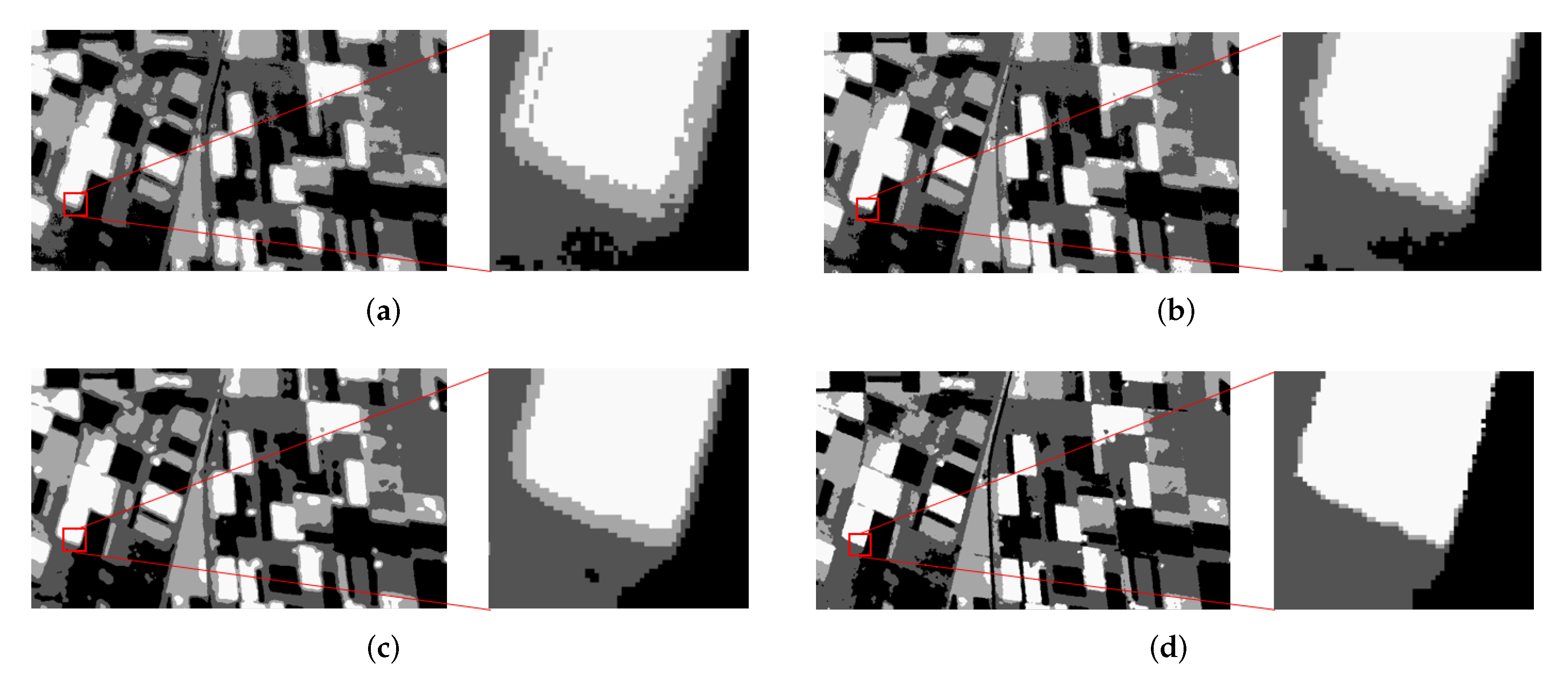
The segmentation results of each algorithm are shown in Figure 13. The results of NS_FCM and FCM_NLS (Figure 13i,j) are relatively clean and accurate. However, there are many misclassified categories at the intersection of different regions. The segmentation results of RFCM_BNL and LBNL_FCM eliminate the isolated pixels and obtain good region conformity. However, RFCM_BNL and LBNL_FCM are prone to misclassification at the edge. The segmentation results of GLR_FCM are cleaner. The serious misclassification at the edge is weakened in GLR_FCM. Some small scale regions can also be segmented, such as roads that appear black being correctly segmented. However, with the noise enhancement, GLR_FCM tends to produce isolated patches when combined with label correction. Figure 14 shows the local detail map of four non-local spatial information FCMs. There is a significant reduction in misclassification at the edge of GLR_FCM.

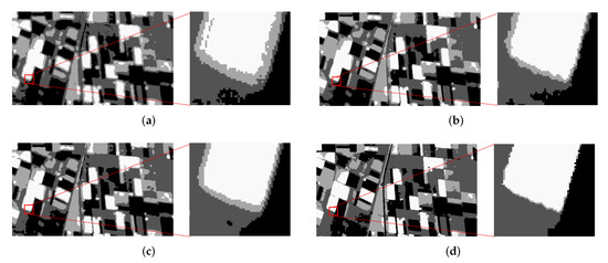
Figure 14. Local detail maps of segmentation results. (a) The result of NS_FCM. (b) The result of RFCM_BNL. (c) The result of LBNL_FCM. (d) The result of GLR_FCM.

3.4.3. Experiment 3: Experiment on the Third Real SAR Image

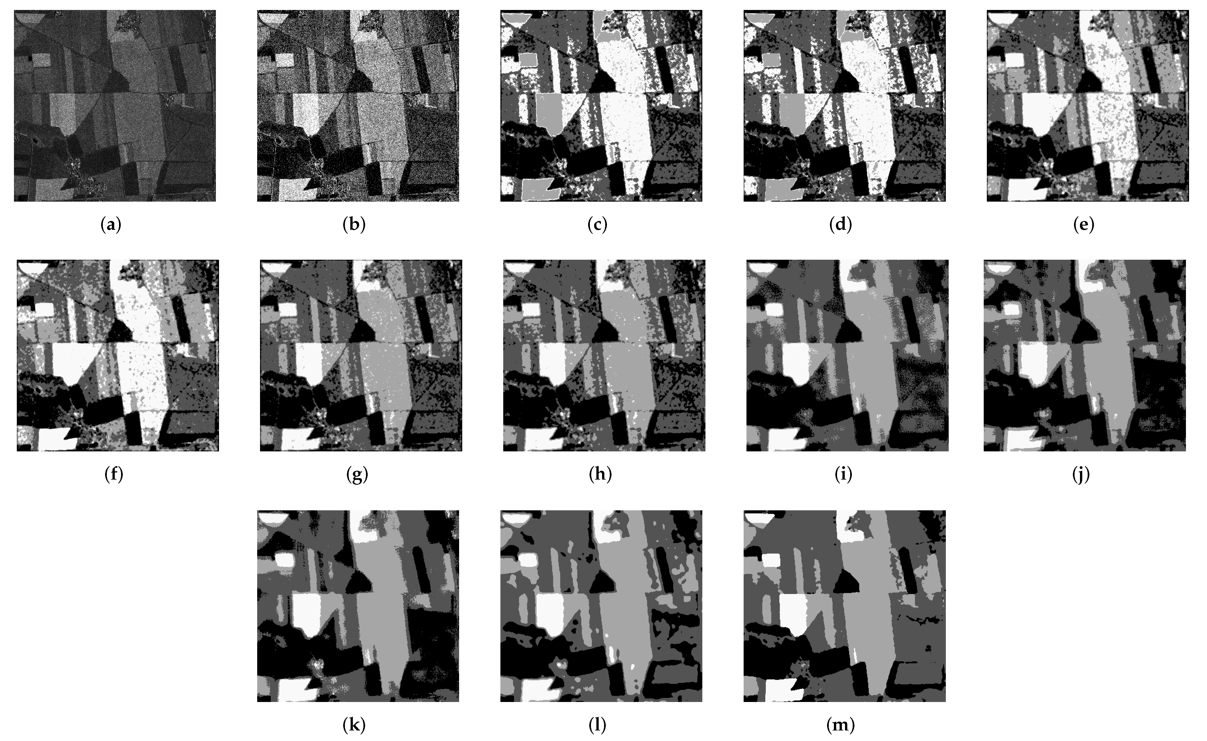
The fourth experiment is performed on a TerraSAR image shown in Figure 15a, which has 5 m spatial resolution and HH polarization in X-band strip imaging mode with 402 × 381 pixels. The SAR image is taken of an area of farmland near the border of Saxony in the German region and includes four categories. Some buildings show high amplitude values, and roads show low amplitude values. These unfavorable factors make it difficult to segment SAR images.

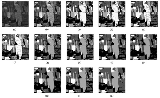
Figure 15. The segmentation results on real image 4. (a) Original image. (b) FCM. (c) FCM_S1. (d) FCM_S2. (e) KFCM_S1. (f) KFCM_S2. (g) EnFCM. (h) FGFCM. (i) FCM_NLS. (j) NS_FCM. (k) RFCM_BNL. (l) LBNL_FCM. (m) GLR_FCM.

The partition results of each algorithm are provided in Figure 15b–m. Obviously, the results of FCM, FCM_S1, FCM_S2 and kernel editions are not satisfactory. Because of the effect of speckle noise, many misclassified pixels, blocks and regions exist. The EnFCM and FGFCM correct the middle area label that is misclassified into highlighted categories in Figure 15c–f. However, the pixels in gray and darker are substantially confused. The addition of NLS_FCM and NS_FCM with non-local information reduces the misclassification, but there is still some isolated noise due to unsuitable Euclidean distance.

Moreover, RFCM_BNL (Figure 15k) obtains good region conformity, but a tiny portion of darker areas is still segmented into black classes. The result of LBNL_FCM significantly weakens the influence of speckle noise, and the best smoothing effect is obtained. GLR_FCM (Figure 15m) is enabled to balance the speckle noise suppression and edge preservation. The region consistency is guaranteed without damaging structure information.

3.4.4. Experiment 4: Experiment on the Fourth Real SAR Image

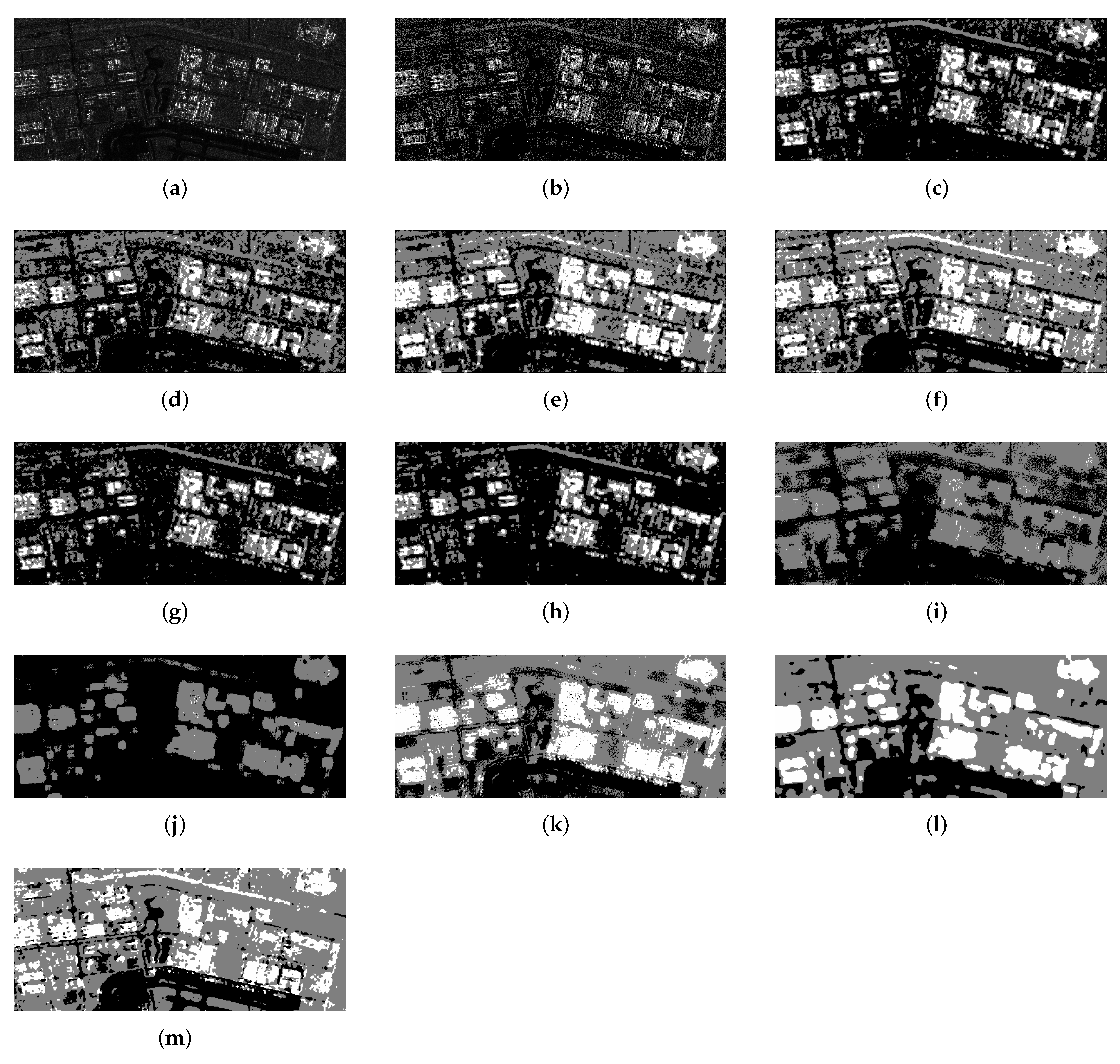
The fifth experiment is a 3 m spatial resolution, 222 × 516 pixels, HH-polarized SAR image taken from GF-3 with the imaging mode of the strip, and this area is located near the Daxing Airport in Beijing. The original image is shown in Figure 16a. The buildings, land, and runways are included in this SAR image; they show in magnitude as highlighted, dark, and black, respectively. Some small areas, such as lakes, also appear black.

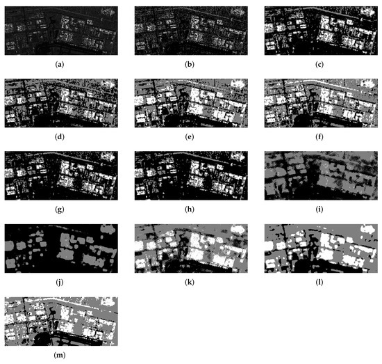
Figure 16. Segmentation results of each algorithm on GaoFen-3 SAR Image. (a) Original image. (b) FCM. (c) FCM_S1. (d) FCM_S2. (e) KFCM_S1. (f) KFCM_S2. (g) EnFCM. (h) FGFCM. (i) FCM_NLS. (j) NS_FCM. (k) RFCM_BNL. (l) LBNL_FCM. (m) GLR_FCM.

Figure 16b–m display the experimental results. As can be seen from Figure 16b the FCM is sensitive to the speckle noise. FCM_S1 and FCM_S2 slightly improve the results. The kernel versions further enhance the separability and homogeneity. However, some speckle blocks are not removed. Due to the complexity of this SAR image, EnFCM, FGFCM, FCM_NLS, and NS_FCM can barely segment correctly. Specifically, EnFCM and FGFCM cannot distinguish the ground and lake. In the results of FCM_NLS and NS_FCM, the building area and ground mix into the same category. This illustrates that the Euclidean distance is unreliable concerning SAR images. Due to the distribution of SAR being considered, RFCM_BNL, LBNL_FCM, and GLR_FCM obtain relatively satisfactory results. The two Bayesian-based FCMs slightly outperform the GLR_FCM in terms of region consistency. However, they are poor in edge localization. Additionally, in terms of structure information preserving, the GLR_FCM surpasses all the algorithms. In Figure 16m, we notice the contour of the lake can be segmented explicitly.

3.5. Sensitivity Analysis to Speckle Noise

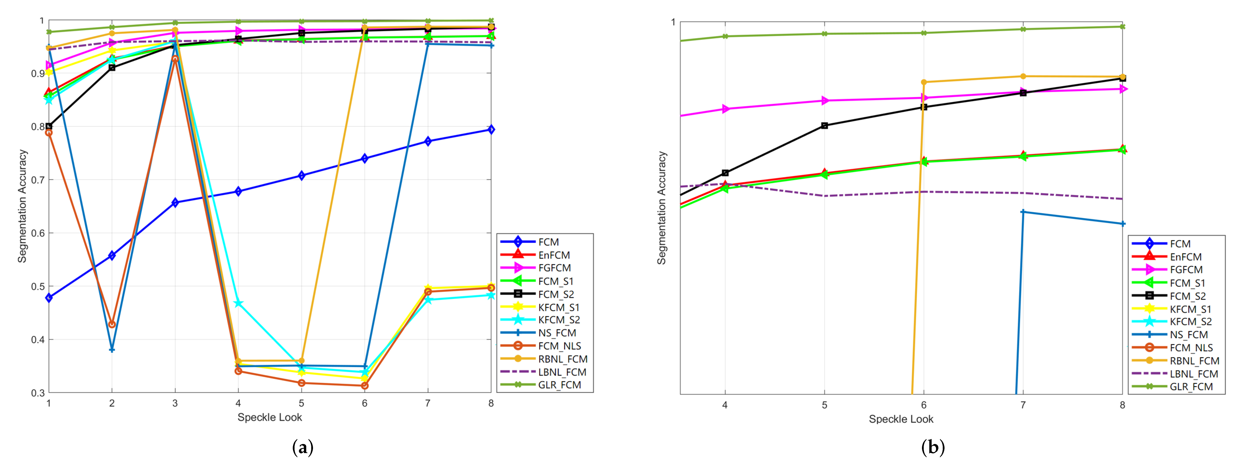
In this section, we evaluate the sensitivity of proposed frameworks to noise intensity by adding different levels of speckle noise to Figure 6a. The SA (%) of different algorithms on images with eight speckle look is shown in Figure 17a. The SA (%) of most methods improves with the weakening of speckle noise. GLR_FCM obtains the best SA (%), which always exceeds 97%. Besides, the stability to different intensity of noise can be observed. LBNL_FCM obtains relatively good SA (%) and is stable for speckle look. The SA (%) of some algorithms fluctuates significantly to the number of speckle look. The variation between the best SA (%) and worst SA (%) exceeds 60%. The partial enlarged view can be seen in Figure 17b.

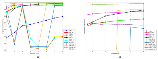
Figure 17. The segmentation accuracy of different algorithms testing on the first simulated SAR image with adding speckle noise of different looks. (a) SA curves of different methods. (b) The partial enlarged view of (a).

3.6. Parameters Analysis and Selection

The non-local search window size $w\times w$ and the square neighborhood size $r\times r$ are two crucial parameters related to the non-local spatial information. In this section, we investigate the optimal parameters on two simulated SAR images (Figure 6a and Figure 9a) for LBNL_FCM and GLR_FCM.

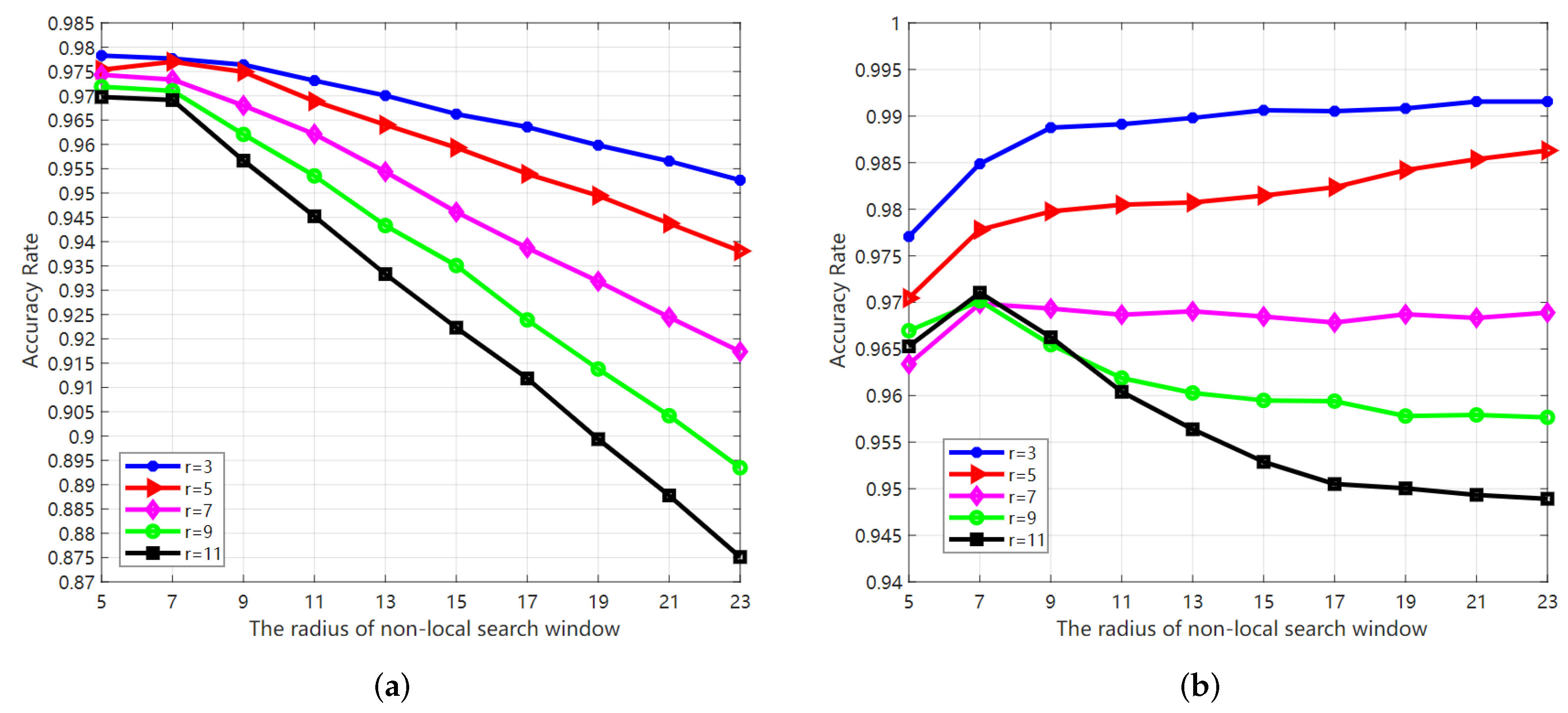
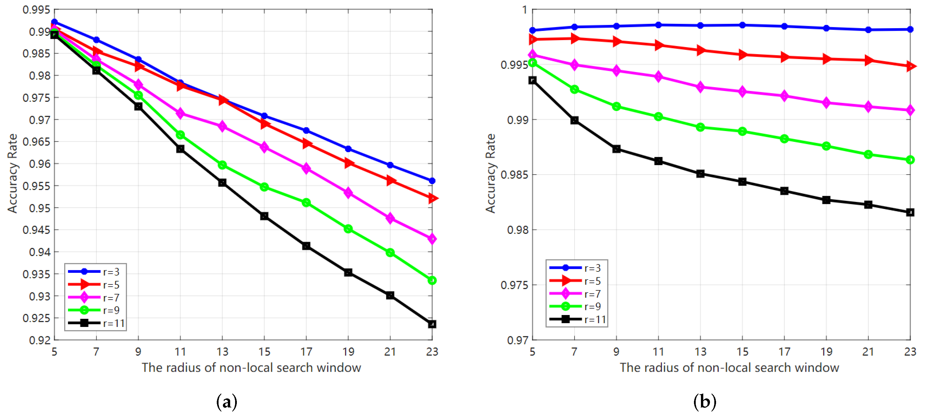
On the first simulated SAR image (Figure 6a), we set the non-local spatial information search window $w=[5,7,9,11,13,15,17,19,21,23]$ and local neighborhood patch $r=[3,5,7,9,11]$. The SA (%) of LBNL_FCM and GLR_FCM on the first simulated SAR image is shown in Figure 18a,b, respectively. From Figure 18a, the SA curve of LBNL_FCM decreases rapidly for ab arbitrary r value when w exceeds 9. One reason for this is that the logarithm transformation reduces the contrast of image amplitude. As the window w expands, more pixels are included to calculate non-local information. Hence, the weight of reliable pixels decreases. The SA (%) curve of GLR_FCM can be seen from Figure 18b. The SA curve of $r=3$ is always higher than others and the accuracy achieves the optimal with $w=23$. Therefore, in the parameter range above, the optimal value for r is 3. On the first simulated SAR image, we set $r=3$, $w=9$ for LBNL_FCM and $r=3$, $w=23$ for GLR_FCM. Figure 19 shows the SA curve of LBNL_FCM and GLR_FCM on the second simulated SAR image. Some similar phenomena can be observed. The curve with local neighborhood size $r=3$ is always more accurate than others.

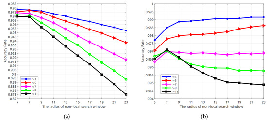
Figure 18. The SA (%) of LBNL_FCM and GLR_FCM carried out on the first simulated SAR image with different sizes of search window $w\times w$ and different sizes of local neighborhood $r\times r$. (a) LBNL_FCM; (b) GLR_FCM.

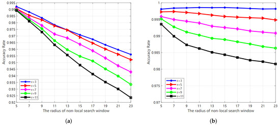
Figure 19. The SA (%) of LBNL_FCM and GLR_FCM carried out on the second simulated SAR image with different sizes of search window $w\times w$ and different sizes of local neighborhood $r\times r$. (a) LBNL_FCM; (b) GLR_FCM.

3.7. Computational Complexity Analysis

The computational complexity of the aforementioned algorithms is given in Table 6. Where N is total pixels, c denotes the number of clustering centers, T represents the iterations, w is the size of the window, r is the size of the non-local search window, s is the size of the neighborhood, W denotes the sliding window for calculating the factor ${\eta }_i$, Q corresponds to the number of gray levels.

Table 6. The computational complexity of algorithms used in this study.

Method	Computational Complexity	Method	Computational Complexity
FCM	$O(N\times c\times T)$	FGFCM	$O(N\times w^2+Q\times c\times T)$
FCM_S1	$O(N\times w^2+N\times c\times T)$	FCM_NLS	$O(N\times r^2\times s^2+N\times c\times T)$
FCM_S2	$O(N\times w^2+N\times c\times T)$	NS_FCM	$O(N\times r^2\times s^2+N\times c\times T)$
KFCM_S1	$O(N\times w^2+N\times c\times T)$	RFCM_BNL	$O(N\times r^2\times s^2+N\times W^2+N\times c\times T)$
KFCM_S2	$O(N\times w^2+N\times c\times T)$	LBNL_FCM	$O(N\times r^2\times s^2+N\times W^2+N\times c\times T)$
EnFCM	$O(N\times w^2+Q\times c\times T)$	GLR_FCM	$O(N\times r^2\times s^2+N\times W^2+N\times c\times T)$

The computational complexity of proposed frameworks LBNL_FCM and GLR_FCM consists of three parts. The first part $O(N\times r^2\times s^2)$ is contributed by the calculation of the non-local spatial information. It is calculated before the iterative process. The second part $O(N\times W^2)$ comes from the calculation of the factor ${\eta }_i$. The third part $O(N\times c\times T)$ is from the iteration process. To sum up, the total computational complexity of LBNL_FCM and GLR_FCM is $O(N\times r^2\times s^2+N\times W^2+N\times c\times T)$.

4. Discussion

In the previous experiments, the effectiveness and robustness of both frameworks are verified. On the simulated SAR images, both algorithms obtain high segmentation accuracy (always exceeding 97%), and some unsupervised assessment indicators, such as $v_{PC}$, $v_{PE}$, also state that the fuzziness of clustering centers in results is reduced. On the real SAR images, LBNL_FCM shows a best region consistency in results compared with the previous algorithms. However, like FCM_NLS, NS_FCM, and RFCM_BNL, artifacts appear at the edge. Except for the factor that the amplitude value is prone to blur near the edge, it is also related to the characteristic of the log-transformed Bayesian metric reducing image contrast. Compared with FCM_NLS and NS_FCM, the results of GLR_FCM show satisfactory region uniformity; no isolated pixels exist. Compared with RFCM_FCM and LBNL_FCM, GLR_FCM can preserve the image details and the edges can be properly defined. The main reason is that the similarity metric constructed by the continued product of the generalized likelihood ratio is a ratio form in mathematical expression. That makes it easy to give a small contribution weight to the patches possessing dissimilar amplitude values with the central pixel, which implies the patches involved in reconstructing the real amplitude of central pixel in Equation (37) are trustworthy. Another feature of the proposed unsupervised FCM frameworks is that the non-local spatial information can be adaptively adjusted. Remarkably, in most previous methods, the relevant parameter is empirically set to a constant. Consequently, edge blurred artefacts are greatly reduced in GLR_FCM.

In addition to the methods involved in this article, there are many methods combining FCM with machine learning. For instance, MFCCM, proposed by Balakrishnan et al. [48], fused the characteristics of deep learning to clustering, and produces a satisfactory fuzzy clustering result. However, the disadvantage of its high computational complexity is also significant. Besides, a semi-supervised method combining CNN and IFCM [49] provided a more in-depth understanding and representation of the data features, although it requires a lot of training data. Compared to the advanced deep learning models, our proposed unsupervised FCM frameworks can quickly and efficiently deliver segmentation results. However, due to the lack of feature extraction and feature expression, the image data cannot be understood in depth.

In the parameter analysis, we confirm that $r=3$ is an optimal value for neighborhood size when measuring patches. However, we found the optimal size of non-local search window of GLR_FCM is $w=23$, which is different from the optimal value $w=15$ explored by other algorithms, such as FCM_NLSL, NS_FCM, and RFCM_BNL. We speculate that, because of the strong inhibition of the GLR_FCM on dissimilar patches, more reliable patches can be obtained by expanding the scope of the search window.

In this paper, an empirical statistical distribution (Nakagami–Reigh) is utilized to describe SAR images. The dedicated model is appropriate for the homogeneous region of the SAR. In other scenarios, such as mountainous areas, urban areas, etc., statistical properties may not be expressed correctly. Besides, The relatively high computational complexity is a limitation of the proposed method. In Section 3.7, the computational complexity was listed ($O(N\times r^2\times s^2+N\times W^2+N\times c\times T)$). From the loss function curve shown in Figure 8 and Figure 10, we can observe that the iterative speed is very fast. Therefore, in the practical application, the computational cost mainly comes from the calculation of the non-local spatial information. In addition, appropriately reducing the number of iterations can also improve the efficiency without reducing the accuracy.

5. Conclusions

To suppress the effect of speckle noise on SAR image segmentation by clustering algorithms, we propose two unsupervised FCM frameworks incorporating non-local spatial information term, named LBNL_FCM and GLR_FCM, respectively. The non-local spatial information in LBNL_FCM and GLR_FCM is obtained by combining the statistical properties of SAR images with Bayesian methods and generalized likelihood ratio methods. Therefore, speckle noise can be suppressed. In both frameworks, a simple membership smoothing strategy complements the local information, allowing the membership of the pixel to be iteratively adjusted towards the most probable class in the local neighborhood. Besides, we add a balance factor to adaptively control the effect of non-local spatial information on the edges, so as to reduce the artifact caused by blurred edges. On the synthetic SAR images, both unsupervised FCM frameworks can obtain 99% segmentation accuracy. Several unsupervised evaluation indicators also indicate LBNL_FCM and GLR_FCM can reduce the fuzziness of the divided clusters in results $(v_{PC}=0.9855,v_{PE}=0.0260)$. Experiments on the real SAR images show that LBNL_FCM can achieve best region consistency, and GLR_FCM can balance noise removal while preserve image detail and reduce edge blur artifacts.

In future research, we will consider combining unsupervised FCM with the characteristic of deep learning to explore intelligent clustering computing.

References

- Rahmani, M.; Akbarizadeh, G. Unsupervised feature learning based on sparse coding and spectral clustering for segmentation of synthetic aperture radar images. IET Comput. Vis. 2015, 9, 629–638. [Google Scholar] [CrossRef]
- Jiao, S.; Li, X.; Lu, X. An Improved Ostu Method for Image Segmentation. In Proceedings of the 2006 8th international Conference on Signal Processing, Guilin, China, 16–20 November 2006; Volume 2. [Google Scholar] [CrossRef]
- Yu, Q.; Clausi, D.A. IRGS: Image Segmentation Using Edge Penalties and Region Growing. IEEE Trans. Pattern Anal. Mach. Intell. 2008, 30, 2126–2139. [Google Scholar] [CrossRef] [PubMed]
- Carvalho, E.A.; Ushizima, D.M.; Medeiros, F.N.; Martins, C.I.O.; Marques, R.C.; Oliveira, I.N. SAR imagery segmentation by statistical region growing and hierarchical merging. Digit. Signal Process. 2010, 20, 1365–1378. [Google Scholar] [CrossRef] [Green Version]
- Xiang, D.; Zhang, F.; Zhang, W.; Tang, T.; Guan, D.; Zhang, L.; Su, Y. Fast Pixel-Superpixel Region Merging for SAR Image Segmentation. IEEE Trans. Geosci. Remote Sens. 2021, 59, 9319–9335. [Google Scholar] [CrossRef]
- Yu, H.; Zhang, X.; Wang, S.; Hou, B. Context-Based Hierarchical Unequal Merging for SAR Image Segmentation. IEEE Trans. Geosci. Remote Sens. 2013, 51, 995–1009. [Google Scholar] [CrossRef]
- Wang, M.; Dong, Z.; Cheng, Y.; Li, D. Optimal segmentation of high-resolution remote sensing image by combining superpixels with the minimum spanning tree. IEEE Trans. Geosci. Remote Sens. 2017, 56, 228–238. [Google Scholar] [CrossRef]
- Ma, F.; Zhang, F.; Xiang, D.; Yin, Q.; Zhou, Y. Fast Task-Specific Region Merging for SAR Image Segmentation. IEEE Trans. Geosci. Remote Sens. 2022, 60, 1–16. [Google Scholar] [CrossRef]
- Zhang, W.; Xiang, D.; Su, Y. Fast Multiscale Superpixel Segmentation for SAR Imagery. IEEE Geosci. Remote Sens. Lett. 2022, 19, 1–5. [Google Scholar] [CrossRef]
- Zhang, X.; Jiao, L.; Liu, F.; Bo, L.; Gong, M. Spectral Clustering Ensemble Applied to SAR Image Segmentation. IEEE Trans. Geosci. Remote Sens. 2008, 46, 2126–2136. [Google Scholar] [CrossRef] [Green Version]
- Mukhopadhaya, S.; Kumar, A.; Stein, A. FCM Approach of Similarity and Dissimilarity Measures with α-Cut for Handling Mixed Pixels. Remote Sens. 2018, 10, 1707. [Google Scholar] [CrossRef] [Green Version]
- Xu, Y.; Chen, R.; Li, Y.; Zhang, P.; Yang, J.; Zhao, X.; Liu, M.; Wu, D. Multispectral image segmentation based on a fuzzy clustering algorithm combined with Tsallis entropy and a gaussian mixture model. Remote Sens. 2019, 11, 2772. [Google Scholar] [CrossRef] [Green Version]
- Madhu, A.; Kumar, A.; Jia, P. Exploring Fuzzy Local Spatial Information Algorithms for Remote Sensing Image Classification. Remote Sens. 2021, 13, 4163. [Google Scholar] [CrossRef]
- Xia, G.S.; He, C.; Sun, H. Integration of synthetic aperture radar image segmentation method using Markov random field on region adjacency graph. IET Radar Sonar Navig. 2007, 1, 348–353. [Google Scholar] [CrossRef]
- Shuai, Y.; Sun, H.; Xu, G. SAR Image Segmentation Based on Level Set With Stationary Global Minimum. IEEE Geosci. Remote Sens. Lett. 2008, 5, 644–648. [Google Scholar] [CrossRef]
- Bao, L.; Lv, X.; Yao, J. Water extraction in SAR Images using features analysis and dual-threshold graph cut model. Remote Sens. 2021, 13, 3465. [Google Scholar] [CrossRef]
- Luo, F.; Zou, Z.; Liu, J.; Lin, Z. Dimensionality reduction and classification of hyperspectral image via multi-structure unified discriminative embedding. IEEE Trans. Geosci. Remote Sens. 2021, 60, 5517916. [Google Scholar] [CrossRef]
- Ma, F.; Gao, F.; Sun, J.; Zhou, H.; Hussain, A. Weakly supervised segmentation of SAR imagery using superpixel and hierarchically adversarial CRF. Remote Sens. 2019, 11, 512. [Google Scholar] [CrossRef] [Green Version]
- Wang, C.; Pei, J.; Wang, Z.; Huang, Y.; Wu, J.; Yang, H.; Yang, J. When Deep Learning Meets Multi-Task Learning in SAR ATR: Simultaneous Target Recognition and Segmentation. Remote Sens. 2020, 12, 3863. [Google Scholar] [CrossRef]
- Colin, A.; Fablet, R.; Tandeo, P.; Husson, R.; Peureux, C.; Longépé, N.; Mouche, A. Semantic Segmentation of Metoceanic Processes Using SAR Observations and Deep Learning. Remote Sens. 2022, 14, 851. [Google Scholar] [CrossRef]
- Zhang, R.; Chen, J.; Feng, L.; Li, S.; Yang, W.; Guo, D. A Refined Pyramid Scene Parsing Network for Polarimetric SAR Image Semantic Segmentation in Agricultural Areas. IEEE Geosci. Remote Sens. Lett. 2022, 19, 1–5. [Google Scholar] [CrossRef]
- Bezdek, J.C.; Ehrlich, R.; Full, W. FCM: The fuzzy c-means clustering algorithm. Comput. Geosci. 1984, 10, 191–203. [Google Scholar] [CrossRef]
- Ahmed, M.N.; Yamany, S.M.; Mohamed, N.; Farag, A.A.; Moriarty, T. A modified fuzzy c-means algorithm for bias field estimation and segmentation of MRI data. IEEE Trans. Med. Imaging 2002, 21, 193–199. [Google Scholar] [CrossRef] [PubMed]
- Chen, S.; Zhang, D. Robust image segmentation using FCM with spatial constraints based on new kernel-induced distance measure. IEEE Trans. Syst. Man Cybern. Part Cybern. 2004, 34, 1907–1916. [Google Scholar] [CrossRef] [Green Version]
- Szilagyi, L.; Benyo, Z.; Szilágyi, S.M.; Adam, H. MR brain image segmentation using an enhanced fuzzy c-means algorithm. In Proceedings of the 25th Annual International Conference of the IEEE Engineering in Medicine and Biology Society (IEEE Cat. No. 03CH37439), Cancun, Mexico, 17–21 September 2003; Volume 1, pp. 724–726. [Google Scholar]
- Cai, W.; Chen, S.; Zhang, D. Fast and robust fuzzy c-means clustering algorithms incorporating local information for image segmentation. Pattern Recognit. 2007, 40, 825–838. [Google Scholar] [CrossRef] [Green Version]
- Krinidis, S.; Chatzis, V. A robust fuzzy local information C-means clustering algorithm. IEEE Trans. Image Process. 2010, 19, 1328–1337. [Google Scholar] [CrossRef] [PubMed]
- Buades, A.; Coll, B.; Morel, J.M. A non-local algorithm for image denoising. In Proceedings of the 2005 IEEE Computer Society Conference on Computer Vision and Pattern Recognition (CVPR’05), San Diego, CA, USA, 20–25 June 2005; Volume 2, pp. 60–65. [Google Scholar]
- Wang, J.; Kong, J.; Lu, Y.; Qi, M.; Zhang, B. A modified FCM algorithm for MRI brain image segmentation using both local and non-local spatial constraints. Comput. Med. Imaging Graph. 2008, 32, 685–698. [Google Scholar] [CrossRef]
- Zhu, L.; Chung, F.L.; Wang, S. Generalized fuzzy c-means clustering algorithm with improved fuzzy partitions. IEEE TRansactions Syst. Man Cybern. Part B Cybern. 2009, 39, 578–591. [Google Scholar]
- Zhao, F.; Jiao, L.; Liu, H. Fuzzy c-means clustering with non local spatial information for noisy image segmentation. Front. Comput. Sci. China 2011, 5, 45–56. [Google Scholar] [CrossRef]
- Zhao, F.; Jiao, L.; Liu, H.; Gao, X. A novel fuzzy clustering algorithm with non local adaptive spatial constraint for image segmentation. Signal Process. 2011, 91, 988–999. [Google Scholar] [CrossRef]
- Feng, J.; Jiao, L.; Zhang, X.; Gong, M.; Sun, T. Robust non-local fuzzy c-means algorithm with edge preservation for SAR image segmentation. Signal Process. 2013, 93, 487–499. [Google Scholar] [CrossRef]
- Ji, J.; Wang, K.L. A robust nonlocal fuzzy clustering algorithm with between-cluster separation measure for SAR image segmentation. IEEE J. Sel. Top. Appl. Earth Obs. Remote Sens. 2014, 7, 4929–4936. [Google Scholar] [CrossRef]
- Wan, L.; Zhang, T.; Xiang, Y.; You, H. A robust fuzzy c-means algorithm based on Bayesian nonlocal spatial information for SAR image segmentation. IEEE J. Sel. Top. Appl. Earth Obs. Remote Sens. 2018, 11, 896–906. [Google Scholar] [CrossRef]
- Kervrann, C.; Boulanger, J.; Coupé, P. Bayesian non-local means filter, image redundancy and adaptive dictionaries for noise removal. In International Conference on Scale Space and Variational Methods in Computer Vision; Springer: Berlin/Heidelberg, Germany, 2007; pp. 520–532. [Google Scholar]
- Deledalle, C.A.; Denis, L.; Tupin, F. How to compare noisy patches? Patch similarity beyond Gaussian noise. Int. J. Comput. Vis. 2012, 99, 86–102. [Google Scholar] [CrossRef] [Green Version]
- Bezdek, J.C. Pattern Recognition with Fuzzy Objective Function Algorithms; Springer: Berlin/Heidelberg, Germany, 1981. [Google Scholar]
- Xie, H.; Pierce, L.; Ulaby, F. Statistical properties of logarithmically transformed speckle. IEEE Trans. Geosci. Remote Sens. 2002, 40, 721–727. [Google Scholar] [CrossRef]
- Goodman, J.W. Some fundamental properties of speckle. JOSA 1976, 66, 1145–1150. [Google Scholar] [CrossRef]
- Oliver, C.; Quegan, S. Understanding Synthetic Aperture Radar Images; SciTech Publishing: Raleigh, NC, USA, 2004. [Google Scholar]
- Shang, R.; Lin, J.; Jiao, L.; Li, Y. SAR Image Segmentation Using Region Smoothing and Label Correction. Remote Sens. 2020, 12, 803. [Google Scholar] [CrossRef] [Green Version]
- Liu, Y.; Zhang, X.; Chen, J.; Chao, H. A validity index for fuzzy clustering based on bipartite modularity. J. Electr. Comput. Eng. 2019, 2019, 2719617. [Google Scholar] [CrossRef] [Green Version]
- Bezdek, J.C. Numerical taxonomy with fuzzy sets. J. Math. Biol. 1974, 1, 57–71. [Google Scholar] [CrossRef]
- Bezdek, J.C. Cluster Validity with Fuzzy Sets; Taylor & Francis: Abingdon, UK, 1973. [Google Scholar]
- Dave, R.N. Validating fuzzy partitions obtained through c-shells clustering. Pattern Recognit. Lett. 1996, 17, 613–623. [Google Scholar] [CrossRef]
- Fukuyama, Y. A new method of choosing the number of clusters for the fuzzy c-mean method. In Proceedings of the 5th Fuzzy Systems Symposium, Kobe, Japan, 3 June 1989; pp. 247–250. [Google Scholar]
- Balakrishnan, N.; Rajendran, A.; Palanivel, K. Meticulous fuzzy convolution C means for optimized big data analytics: Adaptation towards deep learning. Int. J. Mach. Learn. Cybern. 2019, 10, 3575–3586. [Google Scholar] [CrossRef]
- Wang, Y.; Han, M.; Wu, Y. Semi-supervised Fault Diagnosis Model Based on Improved Fuzzy C-means Clustering and Convolutional Neural Network. In Proceedings of the IOP Conference Series: Materials Science and Engineering. IOP Publishing, Shaanxi, China, 8–11 October 2020; Volume 1043, p. 052043. [Google Scholar]
Publisher’s Note: MDPI stays neutral with regard to jurisdictional claims in published maps and institutional affiliations. |
© 2022 by the authors. Licensee MDPI, Basel, Switzerland. This article is an open access article distributed under the terms and conditions of the Creative Commons Attribution (CC BY) license (https://creativecommons.org/licenses/by/4.0/).