Article

The Optimal Phenological Phase of Maize for Yield Prediction with High-Frequency UAV Remote Sensing

1
CAS Engineering Laboratory for Yellow River Delta Modern Agriculture, Institute of Geographic Sciences and Natural Resources Research, Chinese Academy of Sciences, Beijing 100101, China
2
Shandong Dongying Institute of Geographic Sciences, Dongying 257000, China
3
Yusense Information Technology and Equipment (Qingdao) Inc., Qingdao 266000, China
4
Key Laboratory of Ecosystem Network Observation and Modeling, Institute of Geographic Sciences and Natural Resources Research, Chinese Academy of Sciences, Beijing 100101, China
5
College of Resources and Environment, University of Chinese Academy of Sciences, Beijing 100049, China
6
Leibniz Centre for Agricultural Landscape Research (ZALF), 15374 Müncheberg, Germany
7
Department of Crop Sciences, University of Göttingen, 37075 Göttingen, Germany
8
Fine Mechanics and Physics, Changchun Institute of Optics, Chinese Academy of Sciences, Changchun 130033, China
*
Author to whom correspondence should be addressed.
Remote Sens. 2022, 14(7), 1559; https://doi.org/10.3390/rs14071559
Submission received: 21 February 2022 / Revised: 19 March 2022 / Accepted: 22 March 2022 / Published: 24 March 2022
(This article belongs to the Special Issue UAVs in Sustainable Agriculture)

Abstract

:
Unmanned aerial vehicle (UAV)-based multispectral remote sensing effectively monitors agro-ecosystem functioning and predicts crop yield. However, the timing of the remote sensing field campaigns can profoundly impact the accuracy of yield predictions. Little is known on the effects of phenological phases on skills of high-frequency sensing observations used to predict maize yield. It is also unclear how much improvement can be gained using multi-temporal compared to mono-temporal data. We used a systematic scheme to address those gaps employing UAV multispectral observations at nine development stages of maize (from second-leaf to maturity). Next, the spectral and texture indices calculated from the mono-temporal and multi-temporal UAV images were fed into the Random Forest model for yield prediction. Our results indicated that multi-temporal UAV data could remarkably enhance the yield prediction accuracy compared with mono-temporal UAV data (R2 increased by 8.1% and RMSE decreased by 27.4%). For single temporal UAV observation, the fourteenth-leaf stage was the earliest suitable time and the milking stage was the optimal observing time to estimate grain yield. For multi-temporal UAV data, the combination of tasseling, silking, milking, and dough stages exhibited the highest yield prediction accuracy (R2 = 0.93, RMSE = 0.77 t·ha−1). Furthermore, we found that the Normalized Difference Red Edge Index (NDRE), Green Normalized Difference Vegetation Index (GNDVI), and dissimilarity of the near-infrared image at milking stage were the most promising feature variables for maize yield prediction.

1. Introduction

Crop yield is closely related to national food security and personal living standards [1]. Accurate and timely prediction of crop yield before harvest is vital to national food policy-making and precise agricultural management for production improvement [2]. The conventional way to measure crop yield is destructive sampling [3], which is time and labor-consuming for large scales. With the development of sensor technology, remote sensing is now regarded as one of the most effective tools to monitor crop growth and estimate yield [4,5].
Several studies have applied satellite remote sensing data to predict maize (Zea mays L.) yield [6,7,8]. However, satellite data has a fixed and long revisiting period and is susceptible to weather conditions (cloudiness, etc.), which affects the yield prediction’s timeliness and accuracy [9,10]. Owing to its high spatial resolution and flexibility, UAV-based remote sensing has become widely used for predicting crop yields in recent years [11,12]. The multispectral camera is a prevalent choice among UAV sensors because it can simultaneously collect a large amount of vegetation information through images taken at various wavelengths [13]. Spectral reflectance and derived sensing indices have been correlated with the vegetation characteristics incorporating yield information [14]. In such a context, numerous studies have applied UAV-based multispectral remote sensing to provide a fast, profitable, cost-effective, and non-destructive way for yield estimation of various crops such as maize [15,16,17].
Vegetation indices (VIs) calculated by spectral reflectance have been broadly used to estimate the crop growth variables [18,19,20,21]. The study of Xue et al. (2017), reviewing developments and applications of 100 significant Vis, showed that some VIs could offer stable information for yield prediction [22]; however, it is difficult to obtain a robust VIs-based yield prediction model for the whole growth period. Yield is a complex trait that is influenced by a wide range of variables including environmental, genotypic, and agronomic management [23]. In addition, data-driven models, which are often used to predict yield from remote sensing data, cannot fully capture the interactions among those variables. One of the sources of uncertainties in yield predictions is the variability in the relationships between VIs and crop growth variables at distinct phenological stages [2]. For instance, commonly used VIs, such as normalized difference vegetation index (NDVI), may saturate at closed canopy and lose sensitivity during the reproductive stages [24,25,26]. To overcome the abovementioned challenge, some texture variables are combined with the VIs for yield prediction [27,28]. Texture indices (TIs), which describe local effects of spatial dependence and heterogeneity of optical image pixels, are proven to have the capability of providing valuable information and giving a better estimate when combined with spectral indices for maize yield [29].
Machine learning techniques (e.g., random forest (RF), artificial neural network) are generally used for the prediction of crop yield out of remote sensing data as data-driven models [30,31,32]. These machine learning approaches, which handle large amounts of variables, are effective in disentangling complex relationships between numerous remotely sensed information and crop yield via both non-linear and linear approaches [33]. Among these machine learning techniques for yield prediction, RF is one of the most widely used ensemble learning techniques, which combines a large set of decision tree predictors [30,34]. Khanal et al. (2018) used five machine learning algorithms (i.e., RF, support vector machine with radial and linear kernel functions, neural network, gradient boosting model, and cubist) to predict maize yield. After contrastive analysis they concluded that RF exhibited a more accurate yield prediction than the other four methods [35].
Optimizing UAV observation timing is essential for reducing the cost of field campaigns [36]. The growth cycle of maize is relatively short, and the turnover of development stages is rapid, in particular between the six-leaf and blister stages. Therefore, high-frequency crop monitoring is crucial for capturing the rapid development of maize for a promising yield prediction. Most conventional UAV-based monitoring of crop growth is conducted one to four times per growing season [37,38,39], whereas high-frequency UAV observations for maize are not sufficiently researched. Some studies have tried to use multi-temporal UAV data to improve the yield prediction accuracy, resulting in acceptable progress [2,3,40,41,42]. However, the pressing question is the optimal combination between multi-temporal data and the phenological phases to obtain the most accurate yield prediction. In addition, the lead time of yield prediction is critical, since early powerful prediction is more valuable for precision management than that done shortly before harvest. There may be a tradeoff between lead time and accuracy when predicting crop yield. As a result, the earliest suitable observing time for yield prediction could be another major concern. The challenges, as mentioned earlier, have not been thoroughly studied for maize yield prediction to the best of our knowledge.
This study aimed to determine optimal UAV remote sensing observing time (in terms of phenological phase) for maize yield prediction and improve prediction accuracy via high-frequency UAV observations. Our explicit research questions are: (1) which development phase of maize is the optimal observation time for yield prediction? (2) Is the combination of development stages more suitable for the yield prediction of maize compared to single stage and (3) how does the model yield prediction ability improve using multi-temporal UAV data?

2. Materials and Methods

To address the research questions, we established a five steps work-plan:
(1)
UAV-based multispectral observations with high frequency were conducted at nine development phases of maize (Section 2.2.1).
(2)
Pre-processing of UAV multispectral data for the generation of an orthomosaic (Section 2.2.2).
(3)
Calculations of UAV variable implementing in the RF model (Section 2.2.3).
(4)
Performing the RF model for yield prediction using single stage data (Section 2.4.1) and multi-temporal data (Section 2.4.2), respectively.
(5)
Assessing the performance of the prediction models and determining the optimal UAV observation time (Section 2.5) (Figure 1).

2.1. Study Aera

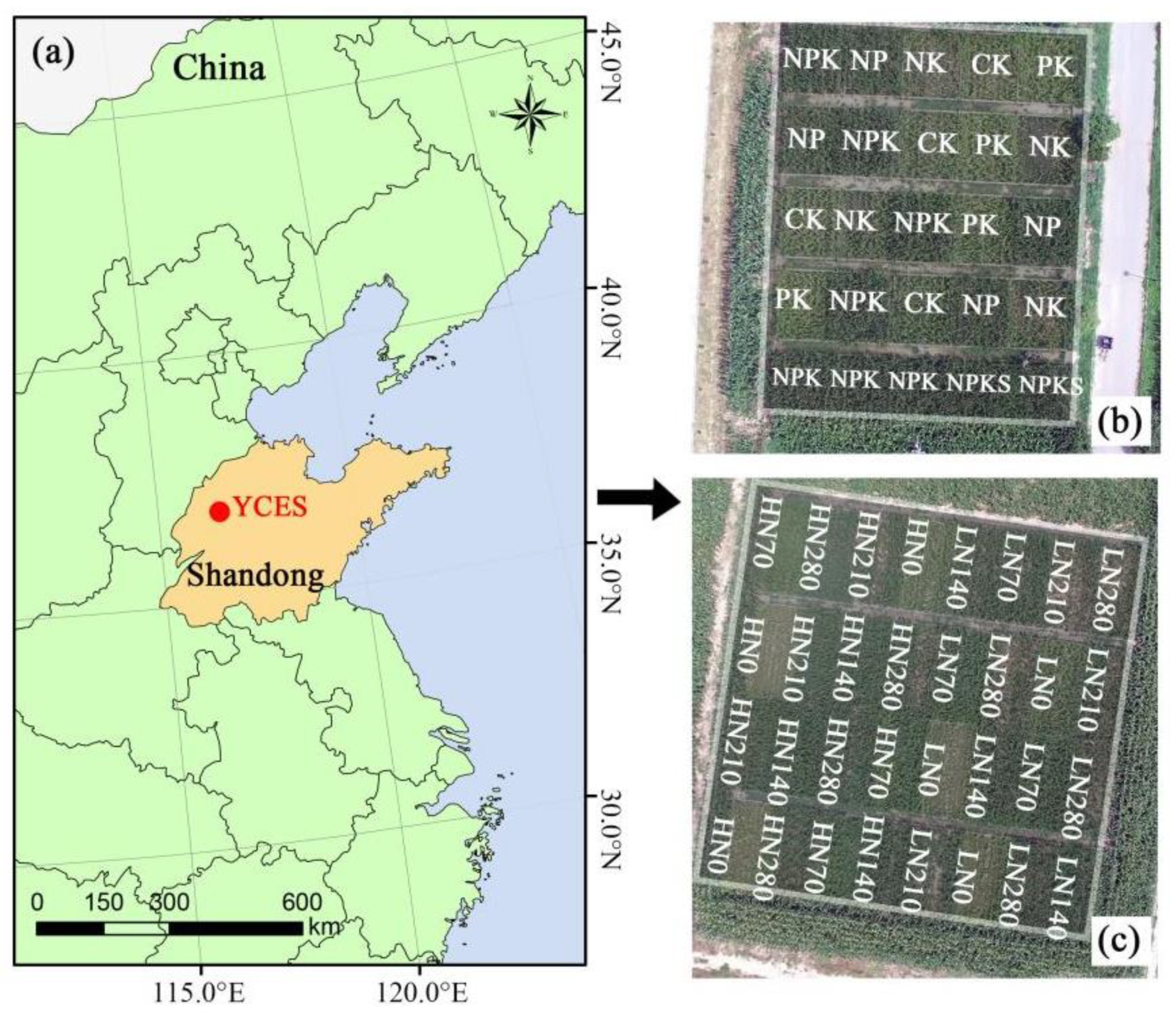
The field experiments were conducted at the Yucheng Comprehensive Experiment Station of the Chinese Academy of Sciences (116.57°E, 36.83°N) in the Shandong Province of China (Figure 2, maps are displayed in GCS_Beijing_1954 Albers projection). The study area has a temperate monsoon climate with an average annual temperate of 13.10 °C. The typical growing season of maize in the study area is from July to September.
UAV remote sensing observations were carried out during the growing season of maize (Zhengdan 958) in the year 2020. Two representative, long-term running experimental fields, the Water Nitrogen Crop Relation (WNCR) experimental site and the Nutrient Balance Experimental Site (NBES) were chosen for the study.
WNCR has been run for 16 years while NBES has been run for about 30 years. In WNCR field, five nitrogen (N)-supply levels (i.e., 0, 70, 140, 210, and 280 kg·N·ha−1) and two irrigation treatments (100 mm and 140 mm, once irrigation at the seventh-leaf stage) were applied. In the NBES field, different N, phosphate (P), and potash (K) fertilizer supply, and residue (S) management were applied. Specification NPK nutrient applications of the two fields are shown in Table 1. Because the growing period of maize is in the rainy season, irrigation for the two fields was done once on 23 July 2020 at the jointing stage of maize. There are 32 plots with a size of 5 m × 10 m in WNCR and 25 plots with a size of 5 m × 6 m in NBES. In total, 57 plots served as samples in this study.

2.2. UAV Multispectral Data Acquisition and Processing

2.2.1. UAV Flight Campaign

A UAV multispectral remote sensing system, which consisted of a four-rotator DJI M200 UAV platform (SZ DJI Technology Co., Shenzhen, China) and a MicaSense RedEdge-M multispectral camera (MicaSense, Inc., Seattle, WA, USA), was used to obtain images of maize. The flights were controlled by the Pix4D Capture software (Pix4D, S.A., Lausanne, Switzerland). The RedEdge-M multispectral camera has five discrete narrow spectral channels centered at 475 nm (blue), 560 nm (green), 668 nm (red), 717 nm (red edge), and 840 nm (near-infrared, NIR).
The flight height was 80 m above ground level with a corresponding ground spatial resolution of 5.45 cm. Sixteen and twelve ground control points (GCPs) distributed evenly within WNCR and NBES, respectively, were used to obtain accurate geographical references and were located with millimeter accuracy by using a Real Time Kinematic (RTK) system (Hi-Target, Inc., Guangzhou, China). The front and side overlaps of the UAV flight missions were 85% and 75%, respectively. The reference panel was captured before and after each UAV flight for radiometric calibration of the obtained multispectral images. All images were taken between 11:00 and 13:00 under a clear sky condition with low wind speed (<5 m·s−1) during the growing period of maize in 2020, that is, the second-leaf, fourth-leaf, six-leaf, fourteenth-leaf, tasseling, silking, milking, dough stage, and maturity [i.e., days of year (DOY) 189, 198, 206, 217, 223, 227, 239, 255, 273, respectively], which were selected in consideration of the critical development stage of maize on yield and the monitoring interval of UAV remote sensing for yield prediction [43,44].

2.2.2. Pre-Processing of UAV-Based Multispectral Remote Sensing Data

The UAV-based multispectral remote sensing data was pre-processed through the PIX4D Mapper software (Pix4D, S.A., Lausanne, Switzerland). First, all multispectral images at the same stage were imported into the Pix4D Mapper. Second, the output coordinate system and the processing options template (AG multispectral) were selected. Then, the radiometric calibration was conducted using the reference panel, and the images were aligned with the ground control points. Finally, automated processing was run in the Pix4D Mapper until exporting the spliced digital orthophoto map. The images obtained at the nine different development phases of maize were pre-processed using the same processing pipeline.

2.2.3. Spectral and Texture Variable Calculations

VIs and TIs were calculated from the UAV multispectral remote sensing orthomosaic. A total of 12 VIs and 8 TIs were selected. The VIs included in this work were based on the previous studies about crop yield prediction, and the corresponding formulations and references were presented in Table 2 [29,45,46,47,48,49].
Eight TIs were calculated in this study, including the mean, variance, homogeneity, contrast, dissimilarity, entropy, second moment, and correlation, which are calculated through the grey level co-occurrence matrix (GLCM) of images of each spectral channel. The CLCM calculation was carried out in the ENVI 5.3 (Exelis Visual Information Solutions, Boulder, CO, USA), and the formulations are listed in Appendix A. The processing window was 3 × 3 pixels. Thus, 52 (12 VIs + 8TIs × 5spectral channels) variables were generated for the yield prediction model. For each variable, we computed the mean values of each plot to represent spectral and textural information at the plot scale.

2.3. Ground Measurement of Maize Yield

At maize maturity, grain yield was measured on 5 October 2020. Two rows of maize plants in each plot were cut for yield measurement considering border effect. Maize kernels were collected and dried at 75 °C until the weight remained constant. Maize yield was calculated as follows,
Yield (kg·m−2) = (M/2) × nrow/(a × b),
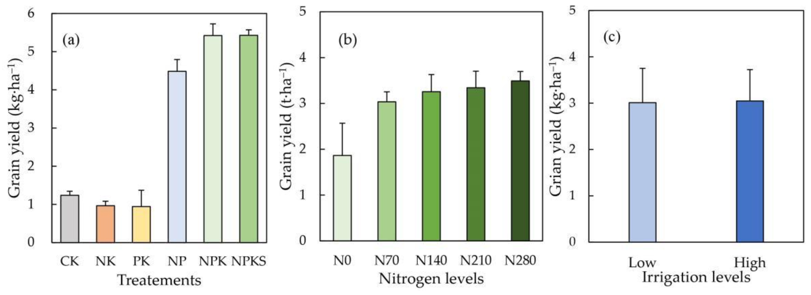
where M (kg) is the weight of kernel for maize collected in each plot (2 rows); nrow is the number of rows for maize (nrow = 9 for both NBES and WNCR); a (m) and b (m) are the width and length of each plot, respectively. Increasing nutrient application levels improved the maize yield significantly (Figure 3). However, irrigation showed a minor effect on the grain yield (Figure 3). It indicates nutrients are the most limiting factor of the grain yield for both experimental sites.

2.4. Data-Driven Model for Yield Prediction

In the present study, the RF algorithm was used to estimate the yield of maize. The prediction models were developed by measured yield and UAV multispectral variables. Two types of models are generated, i.e., the mono-temporal and multi-temporal model, which used UAV data at single and multi-stages, respectively. The RF algorithm was performed in R 4.1.2 (R Core Team, Vienna, Austria) with the open package developed by Breiman et al. [50].

2.4.1. Implementation of Mono-Temporal UAV Data

In this part, nine mono-temporal UAV datasets were used for execution of the yield prediction model, separately. In order to alleviate the effects of information redundancy and noises on model performance, feature variables were initially screened before the model development [51]. For each mono-temporal prediction, 52 UAV remotely-sensed variables were used as RF model inputs to compute the mean decrease in accuracy (MDA) of each predictor variable [34,50]. The MDA of a specific predictor variable indicates the decreased degree of the prediction accuracy when the value of the indicator is turned into a random number. Therefore, it can be regarded as an indicator for assessing the variable importance [45,52,53]. Then the suitability of variables was ranked by the variable importance, and the variation of root mean square errors (RMSE) of the RF model as the number of the input variable increased according to the rank were analyzed.
Theoretically, the number of inputs with the lowest RMSE was regarded as the optimal variable size. However, when determining the appropriate size of the feature variables, the accuracy, robustness, and efficiency of the prediction model should be considered comprehensively [54]. Therefore, the optimal size may not be the ultimate selected size. For example, when the optimal size was large and another smaller input size had a RMSE value roughly equal to the lowest RMSE, the smaller size would be selected, and the corresponding variables were feed-into the RF model. The feature selection procedure was conducted for both experiments (at nine phenological stages). Finally, these selected feature variables were used to develop the mono-temporal-based yield prediction models.
The RF models were developed by optimizing three parameters, including ntree (number of trees to grow), mtry (number of variables randomly sampled as candidates at each split), and nodesize (minimum size of terminal nodes) [2,34]. The optimal model was determined with the lowest RMSE of the prediction result. In addition, the prediction models were validated by the leave-one-out cross validation (LOOCV) method [40,55,56,57]. LOOCV was carried out to avoid the multicollinearity issues by dividing the dataset into training (ntrain = 56) and validation datasets (nvali = 1). LOOCV is a k-fold cross validation, whose k equals to the number of samples (k = n). In this procedure, as the sample size was 57; 56 samples were used as training data while only one sample was used as validation data; the LOOCV process was repeated 57 times with different sample combinations and each model was repeated 1000 times. Although LOOCV is time-consuming, it is recommended for modeling with small sample size [54].

2.4.2. Implementation of Multi-Temporal UAV Data

Based on the prediction results of nine mono-temporal UAV data, models based on the multi-temporal UAV data were developed. First, the nine UAV datasets at distinct maize growth stages were ranked according to their prediction accuracy. The dataset with highest prediction accuracy was ranked first, and the dataset with the lowest prediction accuracy was ranked ninth. Herein, the coefficient of determination (R2) and RMSE of validation (described in Section 2.5) were used as the criterion of prediction accuracy. The multi-temporal UAV datasets were obtained by combing certain mono-temporal UAV datasets, and the combination rule was: the ith group of multi-temporal UAV data was composed of the top (i + 1) ranked UAV datasets. For example, the first group of multi-temporal UAV data includes the UAV datasets ranked first and second. Following such rules, eight groups of multi-temporal UAV datasets were generated.
When developing yield prediction model with multi-temporal UAV data, the same VI or TI calculated from different mono-temporal UAV images were regarded as different variables. As a result, the ith group of multi-temporal UAV data has 52 × (i + 1) variables for model development. For each multi-temporal UAV dataset, feature variables were initially screened using the same method described in Section 2.4.1. Then, the prediction models were developed using the selected UAV variables and were validated by the LOOCV method.

2.5. Performance Analysis

The performance of each yield prediction model was analyzed with the validation results. Two statistical indicators, R2 and RMSE, were used as evaluation metrics to quantify the performances of the models. The calculation formulas of R2 and RMSE are as follows:
R 2 = 1 j = 1 N ( y j y ^ j ) 2 j = 1 N ( y j y - j ) 2
RMSE = 1 N ( y j y ^ j ) 2
where N is the total number of samples, y j and y ^ j denote the jth measured and predicted values of maize yield, respectively; y ¯ is the mean values of measured yield of all plots.

3. Results

3.1. Estimating Maize Yield Using Mono-Temporal UAV Data

3.1.1. Feature Variables Screening of Mono-Temporal UAV Data

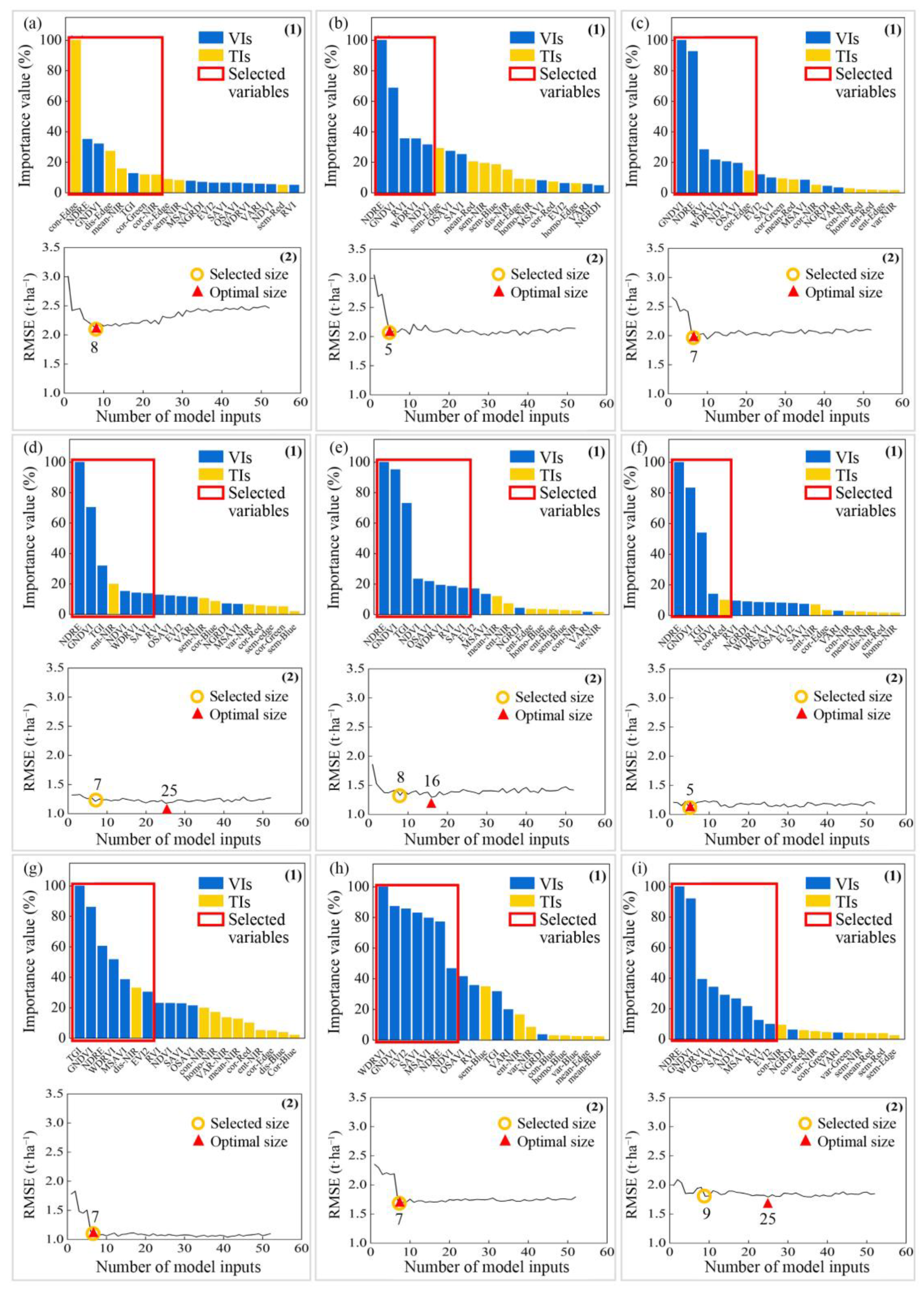
The feature screening of mono-temporal UAV remote sensing data showed that, when the input sizes of models at the fourteenth-leaf, tasseling stages, and maturity were 7, 8, and 9, respectively, their corresponding RMSE values were 1.21, 1.33, and 1.81 t·ha−1, respectively; these RMSE values were roughly equal to the lowest RMSE values of models with input sizes of 25, 16, and 25 (RMSE = 1.18, 1.30, and 1.79 t·ha−1, respectively, Figure 4). In such a context, considering model robustness and importance of inputs (as described in Section 2.4.1), the appropriate numbers of UAV variables for yield prediction based on the mono-temporal UAV data were set to 8, 5, 7, 7, 8, 5, 7, 7, and 9 at the second-leaf, fourth-leaf, sixth-leaf, fourteenth-leaf, tasseling, silking, milking, dough stage, and maturity, respectively.
Our results also showed that the selected UAV variables were different at distinct phenological stages. Except for the second-leaf stage, the spectral indicators (i.e., VIs) played more important roles in yield prediction than the texture indicators (i.e., TIs), as more VIs were selected for modeling and the importance values of VIs were higher than those of TIs (Figure 4(1)). Specifically, among the selected VIs, overall, the normalized difference red edge index (NDRE), green normalized difference vegetation index (GNDVI), and normalized difference vegetation index (NDVI) were the crucial UAV sensing variables for maize yield predication, as these variables were selected at nine development stages (except for the second-leaf stage where NDVI was not included). In terms of the TIs, the NIR and red edge band-derived textures were selected for yield prediction.
In summary, the selected UAV variables and model input sizes were different for each phenological stage, indicating that the appropriate UAV sensing variables for maize yield prediction were considerably affected by maize phenological stages.

3.1.2. Performance of the Prediction Model Using Mono-Temporal UAV Data

The R2 values of yield prediction using mono-temporal UAV data ranged from 0.51 (second-leaf) to 0.86 (milking), and the RMSE values ranged from 2.07 t·ha−1 (second-leaf) to 1.06 t·ha−1 (milking), suggesting the early grain filling is the best phenological stage for yield prediction under the condition of mono-temporal UAV observation (Figure 5). Comparing distinct maize growth stages, yield prediction accuracy followed the order of milking > silking > fourteenth-leaf > tasseling > dough > maturity > six-leaf > fourth-leaf > second-leaf stages (Figure 5). In addition, it should be noted that the prediction accuracies of the four stages including the fourteenth-leaf, tasseling, silking, and milking stages (R2 = 0.78–0.86, RMSE = 1.35–1.06 t·ha−1) were significantly higher than those of the other five stages (R2 = 0.51–0.66, RMSE = 2.07–1.71 t·ha−1) (Figure 5), indicating the period around flowering is the most critical period for the prediction of maize yield.

3.2. Estimating Maize Yield Using Multi-Temporal UAV Data

3.2.1. Generation of Multi-Temporal UAV Groups

In Section 3.1.2, the yield prediction accuracy at nine stages was ranked; thus, eight multi-temporal UAV datasets were generated (Figure 6). Specifically, as the generated UAV sensing variables at each phenological stage was 52, from groups 1 to 8, their UAV variables sizes were 104, 156, 208, 260, 312, 364, 416, and 468, respectively. Hereafter, for the purpose of distinguishing the UAV variables at different stages, the index of jth UAV data was denoted as indexj, where the sequence number of the UAV data was determined according to the order of the data acquisition. For example, NDVI1 denotes the NDVI calculated from the UAV data at the first phenological phase, i.e., the second-leaf stage.

3.2.2. Feature Variables Screening of Multi-Temporal UAV Data

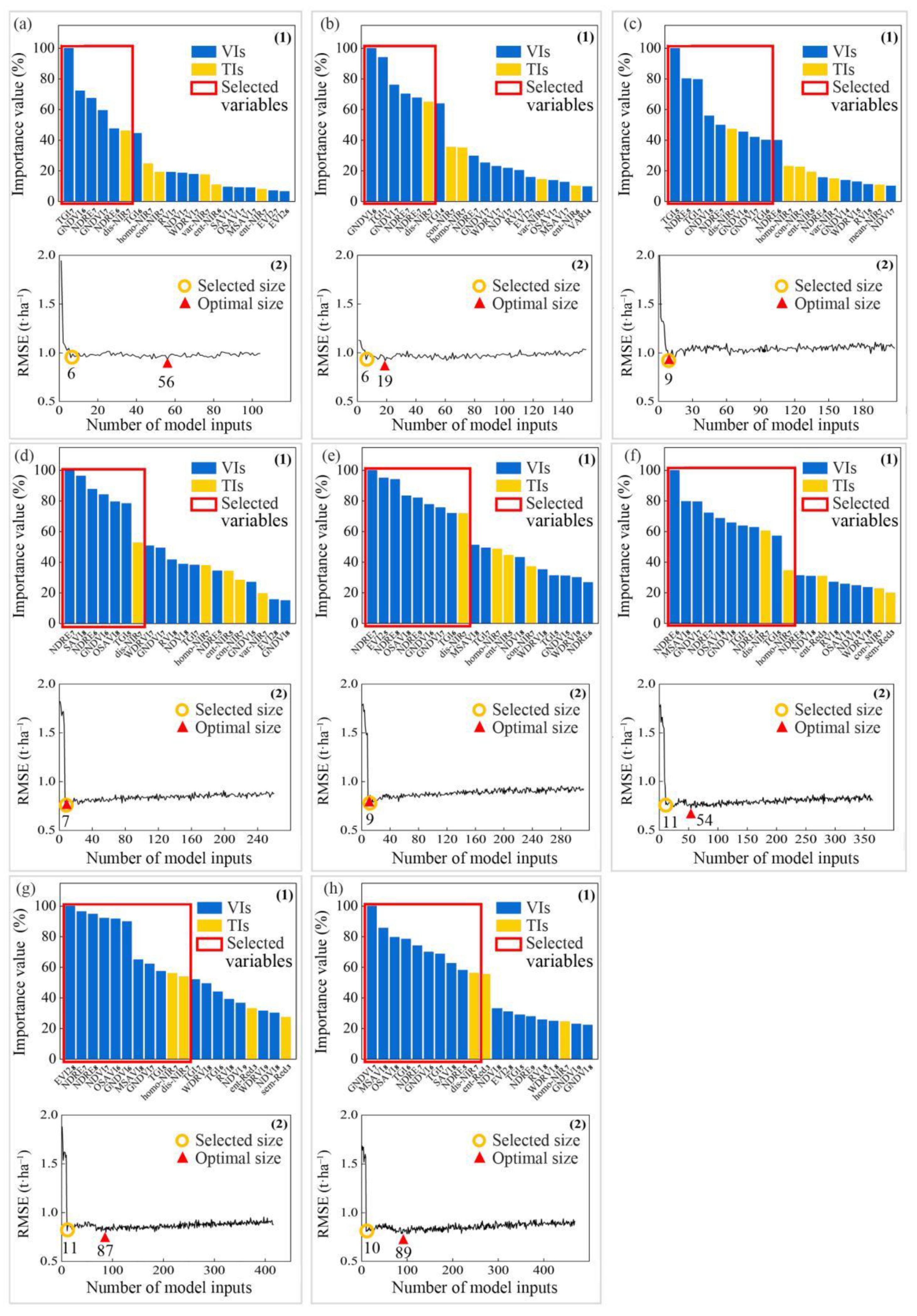
As shown in Figure 7, for the first, second, sixth, seventh, and eighth groups of UAV datasets, the lowest RMSE values were 0.93, 0.92, 0.72, 0.80, and 0.78 t·ha−1, respectively, with corresponding inputs sizes of 56, 19, 54, 87, and 89, respectively (optimal size). Following the rules of Section 2.4.1, the selected input sizes for these four groups were 6, 6, 11, 11, and 10, respectively, as their RMSE values (i.e., 0.95, 0.93, 0.76, 0.81, and 0.81 t·ha−1, respectively) were comparable to the lowest RMSE values. Therefore, the appropriate feature sizes for the eight multi-temporal datasets were determined to be 6, 6, 9, 7, 9, 11, 11, and 10, respectively.
Comparing the selected UAV variables, the number of VIs was obviously higher than TIs, and VIs exhibited higher importance values. This result suggested that VIs were more important than TIs for estimating the maize yield when using multi-temporal UAV data. Among the selected VIs, NDRE and GNDVI were the two variables that were selected in the groups (Figure 7). Whereas the mostly selected TIs was derived from NIR image at the milking stage, and the NIR-based dissimilarly and homogeneity were the two most suitable indicators for yield estimation.

3.2.3. Performance of the Prediction Model Using Multi-Temporal UAV Data

It should be noted that screening in Section 3.2.2 removed UAV variables that were not effective in improving the accuracies of yield prediction models. The UAV data actually used for yield prediction in each group were shown in Figure 6 (the yellow dots); it showed that UAV variables at the second-leaf, fourth-leaf, and sixth-leaf stages were all removed in all groups, indicating that the observations at these three stages were not effective in improving maize yield prediction accuracy.
As displayed in Figure 8, the R2 values of yield prediction using multi-temporal UAV data ranged between 0.89 and 0.93, plus the RMSE values ranged from 0.97 t·ha−1 to 0.77 t·ha−1. From the first to the fourth group, the performance of the prediction model gradually improved. As the number of the used mono-temporal data increases, R2 increases from 0.89 to 0.93, and RMSE decreases from 0.98 t·ha−1 to 0.77 t·ha−1. The best yield prediction was achieved through the fourth group of multi-temporal UAV data which contained the tasseling, silking, milking, and dough stages. We would like to highlight that the UAV data at the tasseling, silking, milking, dough stages were included in the group four to eight (Figure 6), and no obvious improvement was observed from the fourth to eighth groups (Figure 8). These results demonstrated that the combination of tasseling, silking, milking, and dough stages played vital roles in ensuring yield prediction accuracy.

4. Discussion

4.1. Selection of Feature Variables

In this study, VIs and TIs were used to predict maize yield using mono- and multi-temporal remote sensing data. Although this study did not compare the effects of integrating textures in spectral information for yield prediction, the feature selection results showed that both VIs and TIs were selected in yield estimation, particularly for the multi-temporal data. This result proved the importance of TIs in ensuring yield prediction accuracy, which is consistent with previous studies that suggest the integration of TIs into VIs would improve yield estimation accuracy [27,28,29]. As described in the study of Colombo el al. (2003), TIs were able to show the spatial patterns of crop, shadow, and soil pixels [59], so TIs were treated as complementary to overcome the limitation that some VIs may saturate at dense canopy cover and lose sensitivity during the reproductive stages of maize [60,61]. This could explain why TIs were selected in yield prediction.
On the other hand, our results also showed that the VIs contributed more to yield prediction than the TIs, as VIs had higher importance values and more VIs were selected. Yue et al. (2019) concluded that the fusion of VIs and TIs from UAV ultrahigh ground-resolution image could improve the estimation accuracy of above-ground biomass as compared with using only VIs, and they found that the effects of TIs on biomass estimation were highly related to the ground-resolution of images [25]. In this study, the ground-resolution of the multispectral images was around 5 cm, which might not accurately characterize and detect the canopy status to a high accuracy and may then influence the performance of TIs in yield prediction. In future research, we are going to use TIs derived from images with higher ground spatial resolutions to further investigate the effects of image spatial resolution on TIs performance in yield estimation.
The best three spectral indices for maize yield prediction using mono-temporal UAV images were NDRE, GNDVI, and NDVI, which followed the result obtained in Ramos et al. (2020) [45]. When using the multi-temporal data, NDRE and GNDVI also played a predominant role. Moreover, this study selected the 12 commonly-used VIs for crop yield prediction; a future study would investigate the performance of other VIs on yield estimation so as to determine optimal VIs for specific crops and phenological phases. With regard to the TIs, the NIR band derived dissimilarity at the milking stage (i.e., NIR-dis7) was selected in all groups of multi-temporal data. However, other TIs were rarely selected. As mentioned in previous studies, the dissimilarity serves well for edge detection [62,63], which is helpful for object classification when the observed image become complex. Thus, it is significant to calculate TIs using suitable spectral bands and crop development stages for accurately predicting crop yield.

4.2. The Optimal Growth Stage for UAV-Based Maize Yield Prediction

In this study, maize yield prediction using UAV data at the fourteenth-leaf, tasseling, silking, and milking growth stages (DOY 217, 223, 227, and 239, respectively) achieved optimal results with R2 and RMSE around 0.83 and 1.20 t·ha−1. Similar phenological phase have been recognized in other environments and sensors. For example, Fieuzal et al. (2017) concluded that maize yield could be estimated accurately after the flowering stage (DOY 212, stages 60–70, corresponding to the fourteenth-leaf stage in this study) through optical satellite data [64]. Ramos et al. [45], Uno et al. [47], and Martínez et al. [48] successfully forecasted the maize yield with UAV data captured at 50 days after emergence, 66 days after emergence, and 79 days after sowing, respectively, corresponding to the fourteenth-leaf, tasseling, and silking stages in this study. This means the period around flowering and grain filling are most critical for prediction of yield [65]. In addition, yield prediction using UAV data at the milking stage of maize gave the most accurate result with R2 and RMSE of 0.86 and 1.06 t·ha−1. According to the report by IOWA State University, milking stage is the beginning of rapid increase in grain weight [43]. We inferred that the growing status of crop canopy in this period, which can be observed by UAV remote sensing, highly correlated with grain yield. As a result, the milking stage is an ideal candidate for predicting maize yield. In a word, for UAV-based maize yield prediction, fourteenth-leaf and milking stages are the optimal choices, and the former is an earliest suitable observing period while the latter can obtain most accurate predictions.
Early growth stages are less correlated with grain yield. This result is expected as flowering and grain filling are the periods that the grain number and single grain weight is determined [66]. Therefore, earlier growth stages less affect the yield [67]. Furthermore, the demand for water and nutrients in the early growth stage of the crop was not significant, hence the difference in crop growth under different treatments was not adequate. Therefore, the machine learning algorithm implemented at those early development stages could not accurately reflect the difference in yield caused by various nutrient management. Previous studies indicated that the essential condition for developing a suitable data-driven model for yield prediction is that the remote sensing data should be obtained at the growth stage, which plays a decisive role in grain yield [68]. The prediction results with the dough and maturity stage data were also not showing a high performance (R2 around 0.65). During dough and maturity stages, as the assimilates are gradually transferred to the grain, and the chlorophyll content in leaves decreases, the relationships between the canopy spectral reflectance and the grain yield gradually weaken [48], except when an extreme stressor hits the plants, which was not a case in this study. Furthermore, the fully developed reproductive organ layer may cover the canopy traits derived from UAV-based spectral remote sensing which capture a top view [69].

4.3. The Optimal Combination of UAV Observation Time for Maize Yield Prediction

Compared with mono-temporal data, the R2 increased by 8.1% (from 0.86 to 0.93), and RMSE decreased by 27.4% (from 1.06 t·ha−1 to 0.77 t·ha−1) when using multi-temporal data. The significant reduction in RMSE value indicated that the yield prediction accuracy can be improved through the combination of UAV observations at multiple crop growth stages, which is consistent with the conclusion of the previous studies [3,64]. The study of Zhou et al. (2017) demonstrated that the multi-temporal spectral VIs showed a higher correlation with grain yield than the single stage VI [2], as multi-temporal observations are able to provide abundant crop growth information and thus alleviate the biases within mono-temporal observation.
Our results show that the fourth group of multi-temporal data, including the tasseling, silking, milking, and dough stages, was determined to be the optimal UAV observation combination for maize yield prediction, as this combination achieved the highest prediction accuracy with the fewest observations. The recommended observation period played a decisive role in growth and grain yield of maize [43] in other environments. The study of Du et al. (2017) conducted eight consecutive UAV-based observing experiments from June to July 2015 for monitoring wheat growth status, and they found that the accumulative VIs from flowering stage to harvesting had significant relationship with wheat yield [40].
Furthermore, we would like to highlight that the R2 and RMSE values of the fourth group of multi-temporal data changes obviously compared with the third group, where R2 increased from 0.9 to 0.93 and RMSE decreased from 0.93 t·ha−1 to 0.77 t·ha−1, respectively (Figure 8). This variation indicted that the participation of dough stage data in multi-temporal data could improve the accuracy of prediction model significantly, though the prediction result of the model using single dough stage data was not fine (R2 = 0.66 and RMSE = 1.71 t·ha−1). We inferred this could be the evident changes at the dough stage (compared to dough-before stages), which played a crucial role in the RF model.
The R2 and RMSE values among the fourth to eighth groups of multi-temporal data changed slightly, indicating that the feature variables of the fourth multi-temporal data were sufficient in characterizing the relationships between canopy status and grain yield, while extra remotely sensed information was less prone to affect yield prediction accuracy. In addition, it is worth drawing attention to the fact that the selected feature variables of the fifth, sixth, seventh, and eighth groups were relatively stable, all of which were calculated by the UAV data at the tasseling, silking, milking, and dough stages, while the UAV variables at other stages exhibited less importance or were even removed for developing models (Figure 7). Hence, determining the optimal observing time, including growth stage and observing frequency, is essential for improving the UAV remote sensing-based yield prediction accuracy with low time and labor costs.

5. Conclusions

In this study, UAV-based spectral and texture variables at nine phenological stages along with the RF model were used to predict grain yield of maize. Major conclusions are: (1) For mono-temporal UAV observations, the fourteenth-leaf stage was the earliest suitable time and milking stage was the optimal observing time for maize yield prediction. (2) Integration of UAV data at different crop development stages boosted the yield prediction accuracy; and the combination of the UAV observations at tasseling, silking, milking, and dough stages exhibited the highest yield prediction accuracy. (3) NDRE, GNDVI, and near-infrared-based dissimilarity indicators at the milking stage of maize were the suitable variables for grain yield prediction. The finding of this study has theoretical significance and practical value for precision agriculture.

Author Contributions

Conceptualization, B.Y. and W.Z.; Data curation, B.Y., W.Z. and J.L.; Formal analysis, W.Z. and J.L.; Funding acquisition, Z.S.; Methodology, B.Y. and W.Z.; Validation, E.E.R., Z.S. and J.Z.; Writing—original draft, B.Y.; Writing—review & editing, W.Z., E.E.R. and Z.S. All authors have read and agreed to the published version of the manuscript.

Funding

This work was supported by the Strategic Priority Research Program of the Chinese Academy of Sciences (XDA23050102), the Key Projects of the Chinese Academy of Sciences (KJZD-SW-113), the National Natural Science Foundation of China (31870421, 6187030909), and the Program of Yellow River Delta Scholars (2020–2024).

Acknowledgments

Thanks to Guicang Ma, Danyang Yu, and Jiang Bian for UAV flight missions; colleagues of YCES for field measurement.

Conflicts of Interest

The authors declare no conflict of interest.

Appendix A. Calculations of UAV Texture Indices

The calculations of UAV texture indices were expressed as
mean = i j p ( i , j ) i ,
var = i j ( i u ) 2 p ( i , j ) ,
hom = i j 1 1 + ( i j ) 2 p ( i , j ) ,  
con = n = 0 N g 1 n 2 { i = 1 N g j = 1 N g p ( i , j ) | i j | = n } .
dis = n = 1 N g 1 n { i = 1 N g j = 1 N g p ( i , j ) | i j | = n }
ent = i j p ( i , j ) log { p ( i , j ) } ,
sem = i j { p ( i , j ) } 2
cor = i j ( i , j ) p ( i , j ) μ x μ y σ x σ y
where p(i,j)p(i,j) is the (i,j)(i,j)th entry in a normalized gray-tone spatial-dependence matrix P(i,j)/R; px(i) is the ith entry in the marginal-probability matrix obtained by summing the rows; Ng is the number of distinct gray levels in the quantized image; and μx, μy, σx, and σy, are the means and standard deviations of px and py, respectively. Further details of the calculation are available in Haralick et al. (1973) [70].

References

  1. Wang, L.; Tian, Y.; Yao, X.; Zhu, Y.; Cao, W. Predicting grain yield and protein content in wheat by fusing multi-sensor and multi-temporal remote-sensing images. Field Crops Res. 2014, 164, 178–188. [Google Scholar] [CrossRef]
  2. Zhou, X.; Zheng, H.B.; Xu, X.Q.; He, J.Y.; Ge, X.K.; Yao, X.; Cheng, T.; Zhu, Y.; Cao, W.X.; Tian, Y.C. Predicting grain yield in rice using multi-temporal vegetation indices from UAV-based multispectral and digital imagery. ISPRS J. Photogramm. Remote Sens. 2017, 130, 246–255. [Google Scholar] [CrossRef]
  3. Wan, L.; Cen, H.; Zhu, J.; Zhang, J.; Zhu, Y.; Sun, D.; Du, X.; Zhai, L.; Weng, H.; Li, Y.; et al. Grain yield prediction of rice using multi-temporal UAV-based RGB and multispectral images and model transfer-a case study of small farmlands in the South of China. Agric. For. Meteorol. 2020, 291, 108096. [Google Scholar] [CrossRef]
  4. Zhang, H.; Wang, L.; Tian, T.; Yin, J. A Review of Unmanned Aerial Vehicle Low-Altitude Remote Sensing (UAV-LARS) Use in Agricultural Monitoring in China. Remote Sens. 2021, 13, 1221. [Google Scholar] [CrossRef]
  5. Furukawa, F.; Maruyama, K.; Saito, Y.K.; Kaneko, M. Corn Height Estimation Using UAV for Yield Prediction and Crop Monitoring. Unmanned Aer. Veh. Appl. Agric. Environ. 2020, 51–69. [Google Scholar] [CrossRef]
  6. Chivasa, W.; Mutanga, O.; Biradar, C. Application of remote sensing in estimating maize grain yield in heterogeneous African agricultural landscapes: A review. Int. J. Remote Sens. 2017, 38, 6816–6845. [Google Scholar] [CrossRef]
  7. Leroux, L.; Castets, M.; Baron, C.; Escorihuela, M.; Bégué, A.; Seen, D. Maize yield estimation in West Africa from crop process-induced combinations of multi-domain remote sensing indices. Eur. J. Agron. 2019, 108, 11–26. [Google Scholar] [CrossRef]
  8. Yao, F.; Tang, Y.; Wang, P.; Zhang, J. Estimation of maize yield by using a process-based model and remote sensing data in the Northeast China Plain. Phys. Chem. Earth Parts A/B/C 2015, 87–88, 142–152. [Google Scholar] [CrossRef]
  9. Verrelst, J.; Pablo Rivera, J.; Veroustraete, F.; Munoz-Mari, J.; Clevers, J.G.P.W.; Camps-Valls, G.; Moreno, J. Experimental Sentinel-2 LAI estimation using parametric, non-parametric and physical retrieval methods-A comparison. ISPRS J. Photogramm. Remote Sens. 2015, 108, 260–272. [Google Scholar] [CrossRef]
  10. Xie, Q.; Dash, J.; Huete, A.; Jiang, A.; Yin, G.; Ding, Y.; Peng, D.; Christopher, C.H.; Brown, L.; Shi, Y.; et al. Retrieval of crop biophysical parameters from Sentinel-2 remote sensing imagery. Int. J. Appl. Earth Obs. Geoinf. 2019, 80, 187–195. [Google Scholar] [CrossRef]
  11. Nevavuori, P.; Narra, N.; Linna, P.; Lipping, T. Crop Yield Prediction Using Multitemporal UAV Data and Spatio-Temporal Deep Learning Models. Remote Sens. 2020, 12, 4000. [Google Scholar] [CrossRef]
  12. Maimaitijiang, M.; Sagan, V.; Sidike, P.; Hartling, S.; Esposito, F.; Fritschi, F.B. Soybean yield prediction from UAV using multimodal data fusion and deep learning. Remote Sens. Environ. 2020, 237, 111599. [Google Scholar] [CrossRef]
  13. Sankey, J.B.; Sankey, T.T.; Li, J.; Ravi, S.; Wang, G.; Caster, J.; Kasprak, A. Quantifying plant-soil-nutrient dynamics in rangelands: Fusion of UAV hyperspectral-LiDAR, UAV multispectral-photogrammetry, and ground-based LiDAR-digital photography in a shrub-encroached desert grassland. Remote Sens. Environ. 2021, 253, 112223. [Google Scholar] [CrossRef]
  14. Maresma, Á.; Ariza, M.; Martínez, E.; Lloveras, J.; Martínez-Casasnovas, J.A. Analysis of Vegetation Indices to Determine Nitrogen Application and Yield Prediction in Maize (Zea mays L.) from a Standard UAV Service. Remote Sens. 2016, 8, 973. [Google Scholar] [CrossRef] [Green Version]
  15. Hassan, M.A.; Yang, M.; Rasheed, A.; Yang, G.; Reynolds, M.; Xia, X.; Xiao, Y.; He, Z. A rapid monitoring of NDVI across the wheat growth cycle for grain yield prediction using a multi-spectral UAV platform. Plant Sci. 2019, 282, 95–103. [Google Scholar] [CrossRef] [PubMed]
  16. Silva, E.E.; Baio, F.H.R.; Teodoro, L.P.R.; Junior, C.A.; Borges, R.S.; Teodoro, P.E. UAV-multispectral and vegetation indices in soybean grain yield prediction based on in situ observation. Remote Sens. Appl. Soc. Environ. 2020, 18, 100318. [Google Scholar] [CrossRef]
  17. Xie, C.; Yang, C. A review on plant high-throughput phenotyping traits using UAV-based sensors. Comput. Electron. Agric. 2020, 178, 105731. [Google Scholar] [CrossRef]
  18. Yang, M.; Hassan, M.A.; Xu, K.; Zheng, C.; Rasheed, A.; Zhang, Y.; Jin, X.; Xia, X.; Xiao, Y.; He, Z. Assessment of Water and Nitrogen Use Efficiencies Through UAV-Based Multispectral Phenotyping in Winter Wheat. Front. Plant Sci. 2020, 11, 927. [Google Scholar] [CrossRef]
  19. Potgieter, A.B.; George-Jaeggli, B.; Chapman, S.C.; Laws, K.; Suárez Cadavid, L.A.; Wixted, J.; Watson, J.; Eldridge, M.; Jordan, D.R.; Hammer, G.L. Multi-spectral imaging from an unmanned aerial vehicle enables the assessment of seasonal leaf area dynamics of sorghum breeding lines. Front. Plant Sci. 2017, 8, 1532. [Google Scholar] [CrossRef]
  20. Zhang, F.; Zhou, G. Estimation of vegetation water content using hyperspectral vegetation indices: A comparison of crop water indicators in response to water stress treatments for summer maize. BMC Ecol. 2019, 19, 18. [Google Scholar] [CrossRef] [Green Version]
  21. Li, J.; Shi, Y.; Veeranampalayam-Sivakumar, A.N.; Schachtman, D.P. Elucidating sorghum biomass, nitrogen and chlorophyll contents with spectral and morphological traits derived from unmanned aircraft system. Front. Plant Sci. 2018, 9, 1406. [Google Scholar] [CrossRef] [PubMed]
  22. Xue, J.; Su, B. Significant Remote Sensing Vegetation Indices: A Review of Developments and Applications. J. Sens. 2017, 2017, 1353691. [Google Scholar] [CrossRef] [Green Version]
  23. Rotili, D.H.; Voil, P.; Eyre, J.; Serafin, L.; Aisthorpe, D.; Maddonni, G.A.; Rodríguez, D. Untangling genotype x management interactions in multi-environment on-farm experimentation. Field Crops Res. 2020, 255, 107900. [Google Scholar] [CrossRef]
  24. Fu, Y.; Yang, G.; Wang, J.; Song, X.; Feng, H. Winter wheat biomass estimation based on spectral indices, band depth analysis and partial least squares regression using hyperspectral measurements. Comput. Electron. Agr. 2014, 100, 51–59. [Google Scholar] [CrossRef]
  25. Yue, J.; Yang, G.; Tian, Q.; Feng, H.; Xu, K.; Zhou, C. Estimate of winter-wheat above-ground biomass based on UAV ultrahigh-ground-resolution image textures and vegetation indices. ISPRS J. Photogramm. Remote Sens. 2019, 150, 226–244. [Google Scholar] [CrossRef]
  26. Sulik, J.J.; Long, D.S. Spectral considerations for modeling yield of canola. Remote Sens. Environ. 2016, 184, 161–174. [Google Scholar] [CrossRef] [Green Version]
  27. Wang, F.; Yi, Q.; Hu, J.; Xie, L.; Yao, X.; Xu, T.; Zheng, J. Combining spectral and textural information in UAV hyperspectral images to estimate rice grain yield. Int. J. Appl. Earth Obs. Geoinf. 2021, 102, 102397. [Google Scholar] [CrossRef]
  28. Yang, Q.; Shi, L.; Han, J.; Zha, Y.; Zhu, P. Deep convolutional neural networks for rice grain yield estimation at the ripening stage using UAV-based remotely sensed images. Field Crops Res. 2019, 235, 142–153. [Google Scholar] [CrossRef]
  29. Serele, C.Z.; Gwyn, Q.H.J.; Boisvert, J.B.; Pattey, E.; McLaughlin, N.; Daoust, G. Corn yield prediction with artificial neural network trained using airborne remote sensing and topographic data. In Proceedings of the IGARSS 2000, IEEE 2000 International Geoscience and Remote Sensing Symposium, Taking the Pulse of the Planet: The Role of Remote Sensing in Managing the Environmen, Honolulu, HI, USA, 24–28 July 2000. [Google Scholar] [CrossRef]
  30. Zhou, X.; Kono, Y.; Win, A.; Matsui, T.; Tanaka, T.S.T. Predicting within-field variability in grain yield and protein content of winter wheat using UAV-based multispectral imagery and machine learning approaches. Plant Prod. Sci. 2020, 24, 137–151. [Google Scholar] [CrossRef]
  31. Tsouros, D.C.; Bibi, S.; Sarigiannidis, P.G. A Review on UAV-Based Applications for Precision Agriculture. Information 2019, 10, 349. [Google Scholar] [CrossRef] [Green Version]
  32. Klompenburg, T.; Kassahun, A.; Catal, C. Crop yield prediction using machine learning: A systematic literature review. Comput. Electron. Agric. 2020, 177, 105709. [Google Scholar] [CrossRef]
  33. Chlingaryan, A.; Sukkarieh, S.; Whelan, B. Machine learning approaches for crop yield prediction and nitrogen status estimation in precision agriculture: A review. Comput. Electron. Agric. 2018, 151, 61–69. [Google Scholar] [CrossRef]
  34. Breiman, L. Random Forests. Mach. Learn. 2001, 45, 5–32. [Google Scholar] [CrossRef] [Green Version]
  35. Khanal, S.; Fulton, J.; Klopfenstein, A.; Douridas, N.; Shearer, S. Integration of high resolution remotely sensed data and machine learning techniques for spatial prediction of soil properties and corn yield. Comput. Electron. Agric. 2018, 153, 213–225. [Google Scholar] [CrossRef]
  36. Latella, M.; Sola, F.; Camporeale, C. A Density-Based Algorithm for the Detection of Individual Trees from LiDAR Data. Remote Sens. 2021, 13, 322. [Google Scholar] [CrossRef]
  37. Lu, J.; Cheng, D.; Geng, C.; Zhang, Z.; Xiang, Y.; Hu, T. Combining Plant Height, Canopy Coverage and Vegetation Index from UAV-Based RGB Images to Estimate Leaf Nitrogen Concentration of Summer Maize. Biosyst. Eng. 2021, 202, 42–54. [Google Scholar] [CrossRef]
  38. Niu, Y.; Zhang, L.; Zhang, H.; Han, W.; Peng, X. Estimating Above-Ground Biomass of Maize Using Features Derived from UAV-Based RGB Imagery. Remote Sens. 2019, 11, 1261. [Google Scholar] [CrossRef] [Green Version]
  39. Zhu, W.; Sun, Z.; Yang, T.; Li, J.; Peng, J.; Zhu, K.; Li, S.; Gong, H.; Lyu, Y.; Li, B.; et al. Estimating Leaf Chlorophyll Content of Crops via Optimal Unmanned Aerial Vehicle Hyperspectral Data at Multi-Scales. Comput. Electron. Agric. 2020, 178, 105786. [Google Scholar] [CrossRef]
  40. Du, M.; Noguchi, N. Monitoring of Wheat Growth Status and Mapping of Wheat Yield’s within-Field Spatial Variations Using Color Images Acquired from UAV-camera System. Remote Sens. 2017, 9, 289. [Google Scholar] [CrossRef] [Green Version]
  41. Ashapure, A.; Jung, J.; Chang, A.; Oh, S.; Yeom, J.; Maeda, M.; Maeda, A.; Dube, N.; Landivar, J.; Hague, S.; et al. Developing a machine learning based cotton yield estimation framework using multi-temporal UAS data. ISPRS J. Photogramm. Remote Sens. 2020, 169, 180–194. [Google Scholar] [CrossRef]
  42. Song, Y.; Wang, J.; Shan, B. Estimation of Winter Wheat Yield from UAV-Based Multi-Temporal Imagery Using Crop Allometric Relationship and SAFY Model. Drones 2021, 5, 78. [Google Scholar] [CrossRef]
  43. Hanway, J.J. How a corn plant develops. In Special Report; No. 38; Iowa Agricultural and Home Economics Experiment Station Publications at Iowa State University Digital Repository: Ames, IA, USA, 1966. [Google Scholar]
  44. Sánchez, B.; Rasmussen, A.; Porter, J. Temperatures and the growth and development of maize and rice: A review. Glob. Chang. Biol. 2013, 20, 408–417. [Google Scholar] [CrossRef] [PubMed]
  45. Ramos, A.P.M.; Osco, L.P.; Furuya, D.E.G.; Gonçalves, W.N.; Santana, D.C.; Teodoro, L.P.T.; Junior, C.A.S.; Capristo-Silva, G.F.; Li, J.; Baio, F.H.R.; et al. A random forest ranking approach to predict yield in maize with uav-based vegetation spectral indices. Comput. Electron. Agric. 2020, 178, 105791. [Google Scholar] [CrossRef]
  46. Han, L.; Yang, G.; Dai, H.; Xu, B.; Yang, H.; Feng, H.; Li, Z.; Yang, X. Modeling maize above-ground biomass based on machine learning approaches using UAV remote-sensing data. Plant Methods 2019, 15, 10. [Google Scholar] [CrossRef] [PubMed] [Green Version]
  47. Uno, Y.; Prasher, S.O.; Lacroix, R.; Goel, P.K.; Karimi, Y.; Viau, A.; Patel, R.M. Artificial neural networks to predict corn yield from Compact Airborne Spectrographic Imager data. Comput. Electron. Agric. 2005, 47, 149–161. [Google Scholar] [CrossRef]
  48. García-Martínez, H.; Flores-Magdaleno, H.; Ascencio-Hernández, R.; Khalil-Gardezi, A.; Tijerina-Chávez, L.; Mancilla-Villa, O.R.; Vázquez-Peña, M.A. Corn Grain Yield Estimation from Vegetation Indices, Canopy Cover, Plant Density, and a Neural Network Using Multispectral and RGB Images Acquired with Unmanned Aerial Vehicles. Agriculture 2020, 10, 277. [Google Scholar] [CrossRef]
  49. Han, W.; Peng, X.; Zhang, L.; Niu, Y. Summer Maize Yield Estimation Based on Vegetation Index Derived from Multi-temporal UAV Remote Sensing. Trans. Chin. Soc. Agric. Mach. 2020, 51, 148–155. [Google Scholar] [CrossRef]
  50. Random Forests. Available online: https://www.stat.berkeley.edu/~breiman/RandomForests/ (accessed on 7 February 2022).
  51. Li, X.; Long, J.; Zhang, M.; Liu, Z.; Lin, H. Coniferous Plantations Growing Stock Volume Estimation Using Advanced Remote Sensing Algorithms and Various Fused Data. Remote Sens. 2021, 13, 3468. [Google Scholar] [CrossRef]
  52. Li, W.; Niu, Z.; Chen, H.; Li, D.; Wu, M.; Zhao, W. Remote estimation of canopy height and aboveground biomass of maize using high-resolution stereo images from a low-cost unmanned aerial vehicle system. Ecol Ind. 2016, 67, 637–648. [Google Scholar] [CrossRef]
  53. Kuhn, M.; Johnson, K. Applied Predictive Modeling, 1st ed.; Springer: New York, NY, USA, 2013. [Google Scholar]
  54. Zhu, W.; Sun, Z.; Huang, Y.; Yang, T.; Li, J.; Zhu, K.; Zhang, J.; Yang, B.; Shao, C.; Peng, J.; et al. Optimization of multi-source UAV RS agro-monitoring schemes designed for field-scale crop phenotyping. Precis. Agric 2021, 22, 1768–1802. [Google Scholar] [CrossRef]
  55. Michael, K.; Dana, R. Algorithmic stability and sanity-check bounds for leave-one-out cross-validation. Neural Comput. 1999, 11, 1427–1453. [Google Scholar] [CrossRef]
  56. Jurjević, L.; Gašparović, M.; Milas, A.S.; Balenović, I. Impact of UAS Image Orientation on Accuracy of Forest Inventory Attributes. Remote Sens. 2020, 12, 404. [Google Scholar] [CrossRef] [Green Version]
  57. Féret, J.; François, C.; Gitelson, A.; Asner, G.; Barry, K.; Panigada, C.; Richardson, A.; Jacquemoud, S. Optimizing spectral indices and chemometric analysis of leaf chemical properties using radiative transfer modeling. Remote Sens. Environ. 2011, 115, 2742–2750. [Google Scholar] [CrossRef] [Green Version]
  58. Almeida, C.T.; Galvão, L.S.; Aragão, L.E.; Ometto, J.P.H.B.; Jacon, A.D.; Pereira, F.R.S.; Sato, L.Y.; Lopes, A.P.; Graça, P.M.L.; Silva, A.; et al. Combining LiDAR and hyperspectral data for aboveground biomass modeling in the Brazilian Amazon using different regression algorithms. Remote Sens. Environ. 2019, 232, 111323. [Google Scholar] [CrossRef]
  59. Colombo, R.; Bellingeri, D.; Fasolini, D.; Marino, C.M. Retrieval of leaf area index in different vegetation types using high resolution satellite data. Remote Sens. Environ. 2003, 86, 120–131. [Google Scholar] [CrossRef]
  60. Sun, H.; Li, M.Z.; Zhao, Y.; Zhang, Y.E.; Wang, X.M.; Li, X.H. The spectral characteristics and chlorophyll content at winter wheat growth stages. Spectrosc. Spectr. Anal. 2010, 30, 192–196. [Google Scholar] [CrossRef]
  61. Yue, J.; Feng, H.; Yang, G.; Li, Z. A comparison of regression techniques for estimation of above-ground winter wheat biomass using near-surface spectroscopy. Remote Sens. 2018, 10, 66. [Google Scholar] [CrossRef] [Green Version]
  62. Treitz, P.M.; Howarth, P.J.; Filho, O.R.; Soulis, E.D. Agricultural Crop Classification Using SAR Tone and Texture Statistics. Can. J. Remote Sens. 2000, 26, 18–29. [Google Scholar] [CrossRef]
  63. Wan, S.; Chang, S.H. Crop classification with WorldView-2 imagery using Support Vector Machine comparing texture analysis approaches and grey relational analysis in Jianan Plain, Taiwan. Int. J. Remote Sens. 2019, 40, 8076–8092. [Google Scholar] [CrossRef]
  64. Fieuzal, R.; Sicre, C.M.; Baup, F. Estimation of corn yield using multi-temporal optical and radar satellite data and artificial neural networks. Int. J. Appl. Earth Obs. Geoinf. 2017, 57, 14–23. [Google Scholar] [CrossRef]
  65. Ji, Z.; Pan, Y.; Zhu, X.; Wang, J.; Li, Q. Prediction of Crop Yield Using Phenological Information Extracted from Remote Sensing Vegetation Index. Sensors 2021, 21, 1406. [Google Scholar] [CrossRef] [PubMed]
  66. LÜ, G.; Wu, Y.; Bai, W.; Ma, B.; Wang, C.; Song, J. Influence of High Temperature Stress on Net Photosynthesis, Dry Matter Partitioning and Rice Grain Yield at Flowering and Grain Filling Stages. J. Integr. Agric. 2013, 12, 603–609. [Google Scholar] [CrossRef]
  67. Széles, A.V.; Megyes, A.; Nagy, J. Irrigation and nitrogen effects on the leaf chlorophyll content and grain yield of maize in different crop years. Agric. Water Manag. 2012, 107, 133–144. [Google Scholar] [CrossRef]
  68. Qader, S.H.; Dash, J.; Atkinson, P.M. Forecasting wheat and barley crop production in arid and semi-arid regions using remotely sensed primary productivity and crop phenology: A case study in Iraq. Sci. Total Environ. 2018, 613, 250–262. [Google Scholar] [CrossRef] [Green Version]
  69. Li, W.; Jiang, J.; Weiss, M.; Madec, S.; Tison, F.; Philippe, B.; Comar, A.; Baret, F. Impact of the reproductive organs on crop BRDF as observed from a UAV. Remote Sens. Environ. 2021, 259, 112433. [Google Scholar] [CrossRef]
  70. Haralick, R.M.; Shanmugam, K.; Dinstein, I. Textural features for image classification. IEEE Trans. Syst. Man. Cybern. 1973, SMC-3, 610–621. [Google Scholar] [CrossRef] [Green Version]
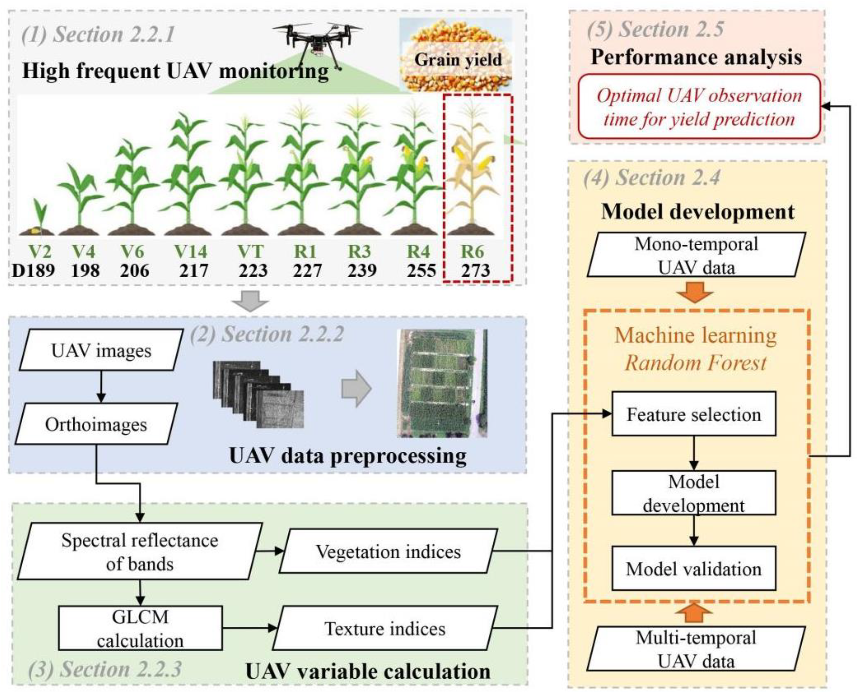
Figure 1. A brief framework for maize yield prediction in this study (GLCM = grey level co-occurrence matrix; V2, V4, V6, V14, VT, R1, R3, R4, and R6 are the second-leaf, fourth-leaf, six-leaf, fourteenth-leaf, tasseling, silking, milking, dough stage, and maturity, respectively; UAV = unmanned aerial vehicle; D = DOY = day of year).
Remotesensing 14 01559 g001
Figure 2. (a) Location of the YCES of the Chinese Academy of Sciences; (b) overview of NBES field; (c) overview of WNCR field. (N, P, K denote nitrogen, phosphate, and potash fertilizer, respectively, and S denotes returning all straw to field; CK is no NPK fertilizer; N0, N70, N140, N210, and N280 denote that 0, 70, 140, 210, and 280 kg·N·ha−1 were applied for each growing season, respectively; L and H denote 100 mm and 140 mm irrigation, respectively).
Remotesensing 14 01559 g002
Figure 3. The observed grain yield at varying nutrient treatments: (a) NBES plots, WNCR plots across various (b) nitrogen and (c) irrigation levels.
Remotesensing 14 01559 g003
Figure 4. (1) Importance values of the top 20 ranked variables for the yield prediction model and (2) RMSE variation (t·ha−1) as the size of inputs increases when using each of the nine mono-temporal UAV data: (a) second-leaf, (b) fourth-leaf, (c) sixth-leaf, (d) fourteenth-leaf, (e) tasseling, (f) silking, (g) milking, (h) dough stage, and (i) maturity. The importance values were normalized by the value of the first ranked variable for each stage [58]. TIs of the images calculated using blue, green, red, red edge, and NIR bands are denoted as TI-Blue, TI-Green, TI-Red, TI-Edge, and TI-NIR, respectively. con = contrast, dis = dissimilarity, cor = correlation, sem = second moment, ent = entropy, homo = homogeneity, var = variance.
Remotesensing 14 01559 g004
Figure 5. Yield prediction accuracy using different mono-temporal UAV data: (a) R2 and (b) RMSE (t·ha−1) values.
Remotesensing 14 01559 g005
Figure 6. The compositions of the eight multi-temporal UAV datasets. (Red/grey denotes mono-temporal datasets are included/excluded in the multi-temporal datasets; yellow dots denote the selected mono-temporal datasets after feature variables screening, which was described in the following Section 3.2.2).
Remotesensing 14 01559 g006
Figure 7. (1) Importance values of the top 20 ranked variables for the prediction model and (2) RMSE variation (t·ha−1) as the size of inputs increases when using each of the eight groups of multi-temporal UAV data: (a) group 1; (b) group 2; (c) group 3; (d) group 4; (e) group 5; (f) group 6; (g) group 7; (h) group 8. The subscript of the variable denotes the sequence number of the used UAV data, which is determined according to the order of the data acquisition; for example, NDVI1 denotes NDVI generated from the first experiment, i.e., the second-leaf stage. dis = dissimilarity, homo = homogeneity, con = contrast, var = variance, ent = entropy, sem = second moment.
Remotesensing 14 01559 g007
Figure 8. Yield prediction accuracy using different multi-temporal UAV data: (a) R2 and (b) RMSE (t·ha−1) values.
Remotesensing 14 01559 g008
Table 1. NPK nutrient treatments in the WNCR and NBES fields.
TreatmentsFertilizer N-P-K (kg·ha−1)TreatmentsFertilizer N-P-K (kg·ha−1)
CK 10-0-0N0 0-120-80
NK245-0-120N70 70-120-80
NP245-30-0N140 140-120-80
PK0-30-120N210 210-120-80
NPK
NPKS 2
245-30-120
245-30-120
N280
/
280-120-80
/
1 CK = no fertilizer (average initial nutrient content for 0–60 cm soil layer: soil organic carbon content = 0.81%, total N = 0.063%, available N, P, and K are 39.72, 3.53, and 95.40 mg·kg−1, respectively). 2 N, P, K denote nitrogen, phosphate, and potash fertilizer, respectively; S denotes returning the whole straw of each plot into the soil.
Table 2. Formulations and references of the selected vegetation indices in this study.
Vegetation IndicesFormulationsReferences
Normalized difference vegetation indexNDVI = (Rnir − Rred)/(Rnir + Rred)[45]
Normalized difference red edge indexNDRE = (Rnir − Rrededge)/(Rnir + Rrededge)[45]
Green normalized difference vegetation indexGNDVI = (Rnir − Rgreen)/(Rnir + Rgreen)[45]
Normalized green-red difference IndexNGRDI = (Rgreen − Rred)/(Rgreen + Rred)[46]
Simple ratioSR = Rnir/Rred[47]
Triangular greenness indexTGI = Rgreen − 0.39Rred − 0.61Rblue[48]
Wide dynamic range vegetation indexWDRVI = (0.1Rnir − Rred)/(0.1Rnir + Rred)[48]
Visible atmospherically resistant indexVARI = (Rgreen − Rred)/(Rgreen + Rred − Rblue)[48]
Soil adjusted vegetation indexSAVI = 1.5(Rnir − Rred)/(Rnir + Rred + 0.5)[29]
Optimized soil adjusted vegetation indexOSAVI = 1.16(Rnir − Rred)/(Rnir + Rred + 0.16)[49]
Enhanced vegetation index 2EVI2 = 2.5(Rnir − Rred)/(Rnir + 2.4Rred + 1)[49]
Modified soil adjusted vegetation index 2 MSAVI 2 = 0.5 [ ( 2 R nir   + 1 ) ( 2 R nir 1 ) 2 + 8 ( R nir R red ) ] [49]
Note: Rnir, Rred, Rrededge, Rblue, and Rgreen denote the spectral reflectance of the near-infrared, red, rededge, blue, and green bands, respectively.
Publisher’s Note: MDPI stays neutral with regard to jurisdictional claims in published maps and institutional affiliations.