
Land Subsidence in the Texas Coastal Bend: Locations, Rates, Triggers, and Consequences


 , , and
Abstract
:
1. Introduction
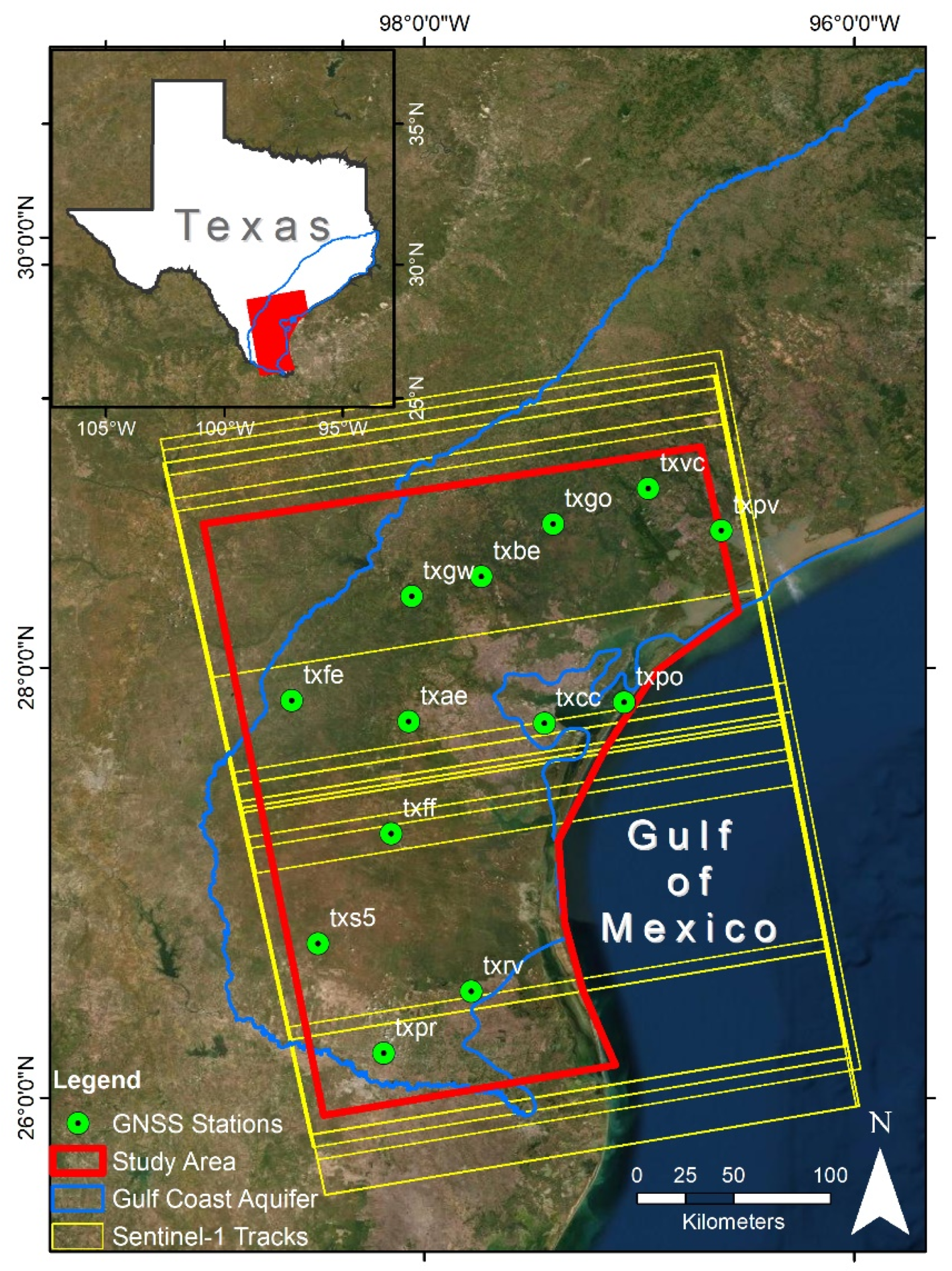
2. Study Area
3. Data
4. Methods
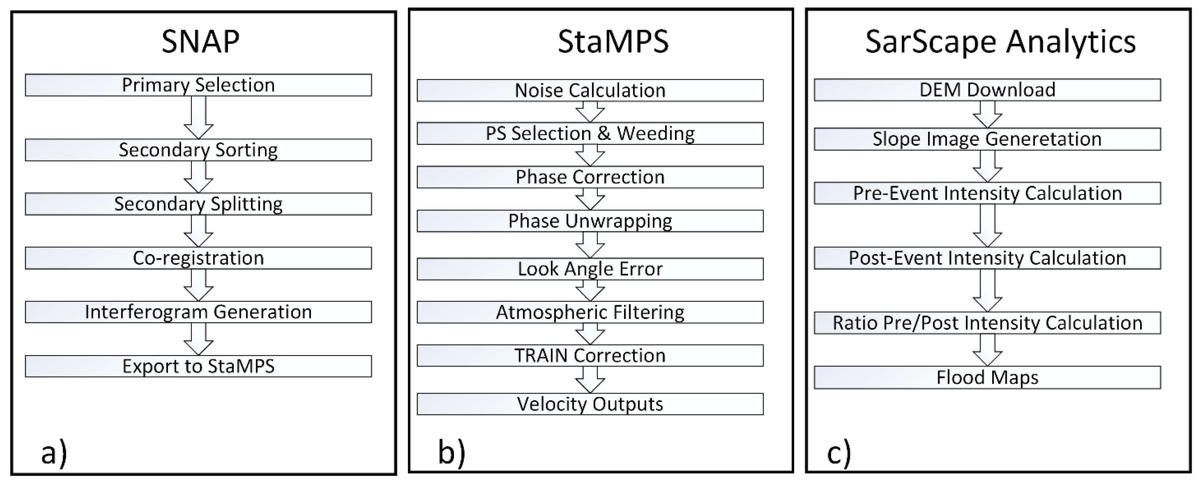
4.1. Mapping Land Subsidence Rates and Locations
- Secondary image preparation: The available SAR data within the project folder is separated into individual folders by acquisition date.
- Secondary splitting: The secondary images are split into the correct area of interest and orbital corrections are applied.
- Co-registration and interferogram generation: The SAR data is co-registered, producing a set of interferograms with the topographic phase removed, and separate files are prepared for the execution of StaMPS analysis.
- StaMPS export: The interferograms are converted into binary files that are compatible as StaMPS inputs.
4.2. InSAR-GNSS Validation
4.3. Mapping Flooded Areas
5. Results
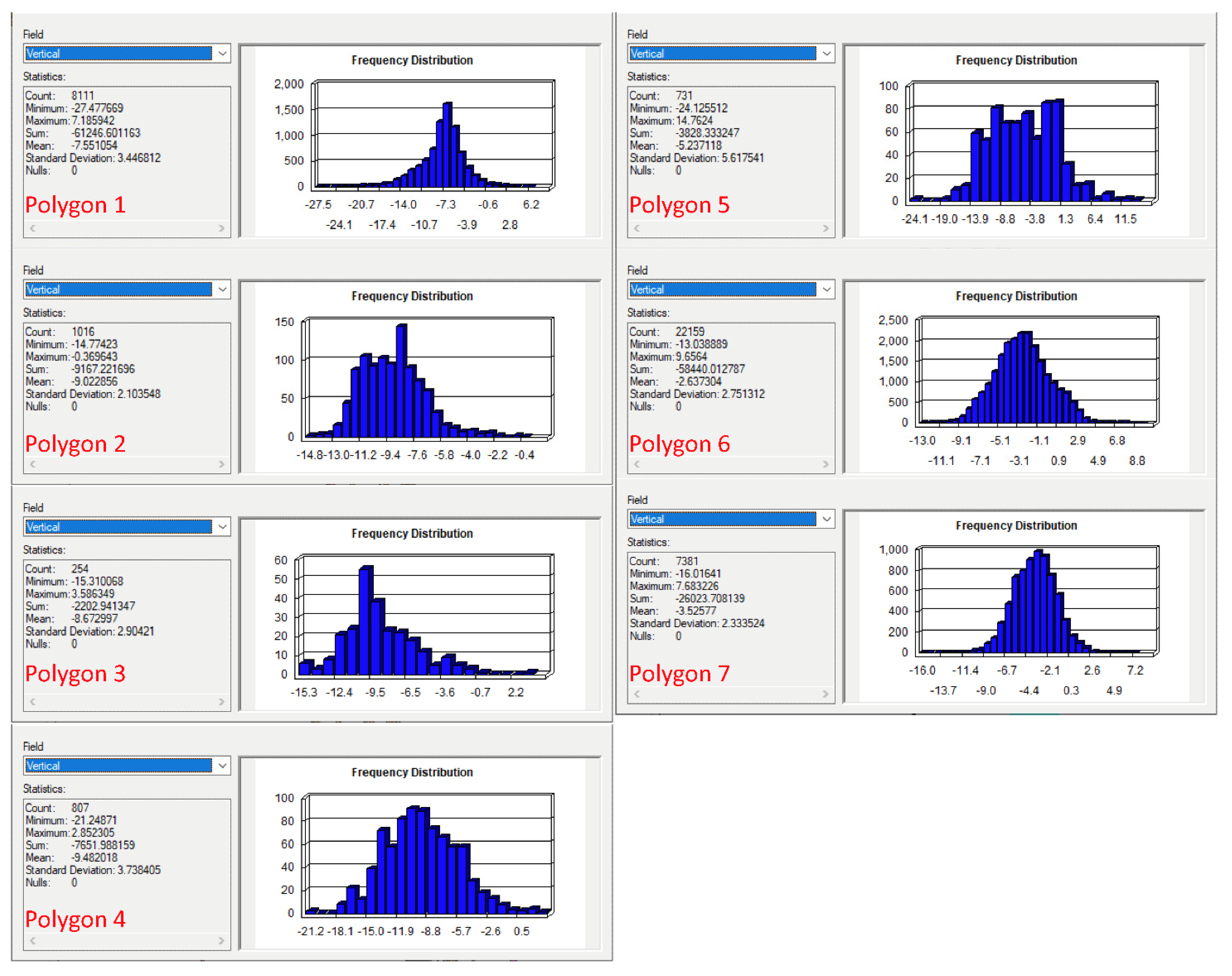
5.1. Land Subsidence Rates in the Texas Coastal Bend
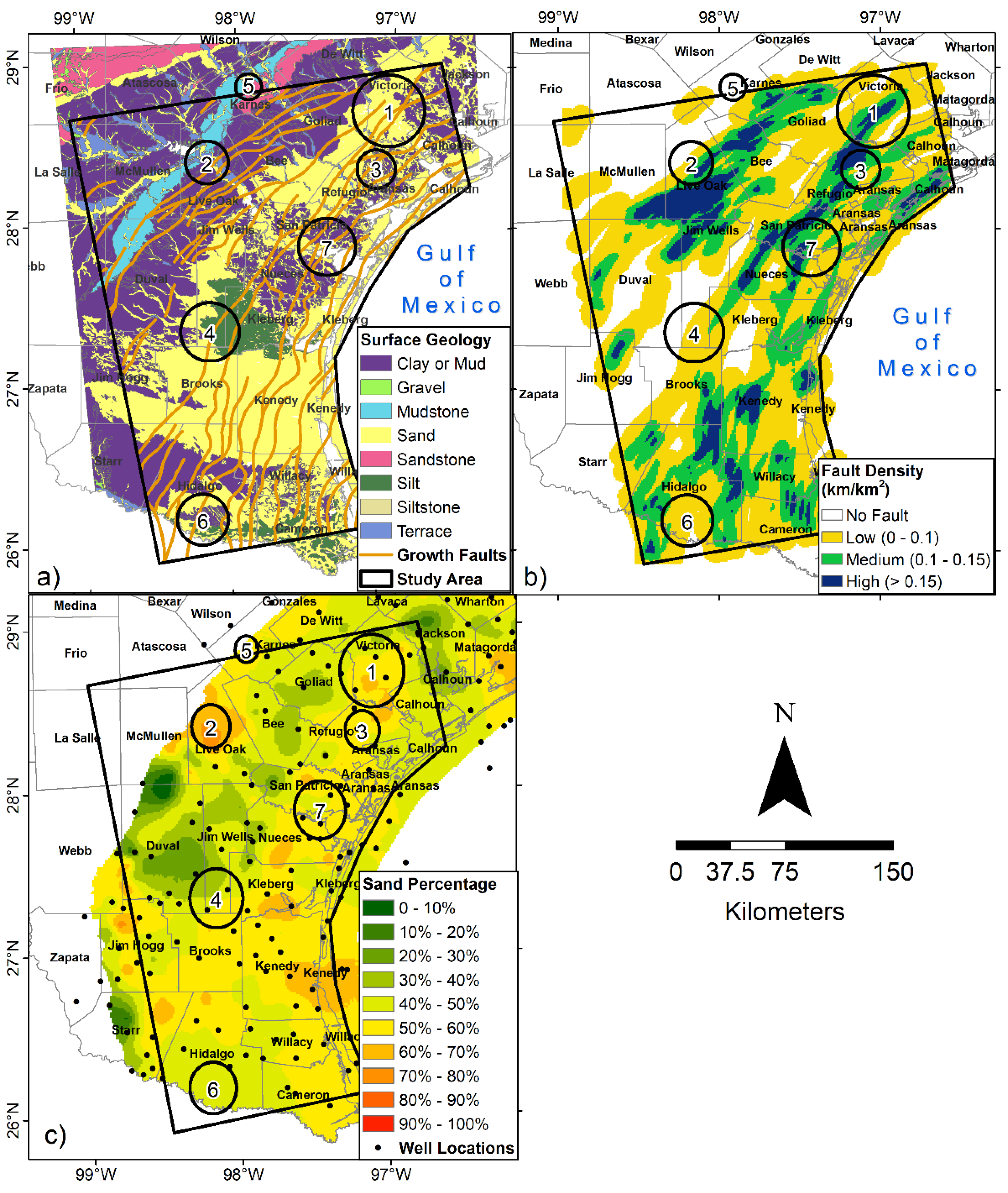
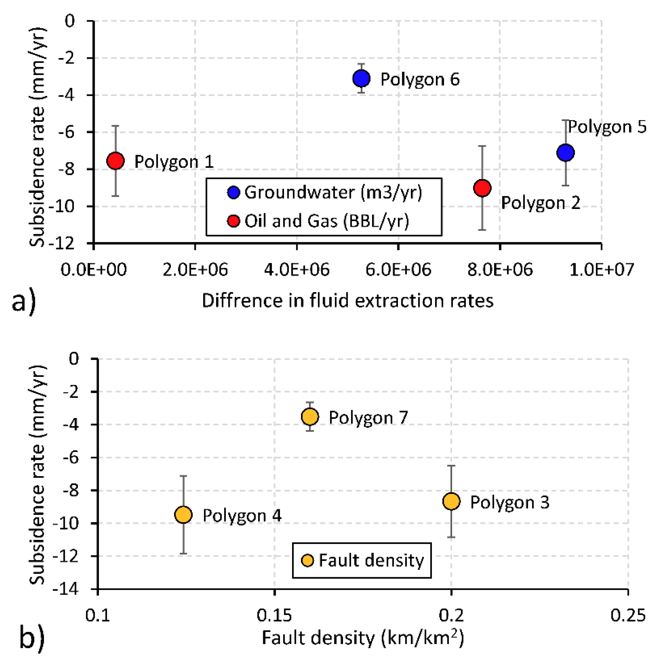
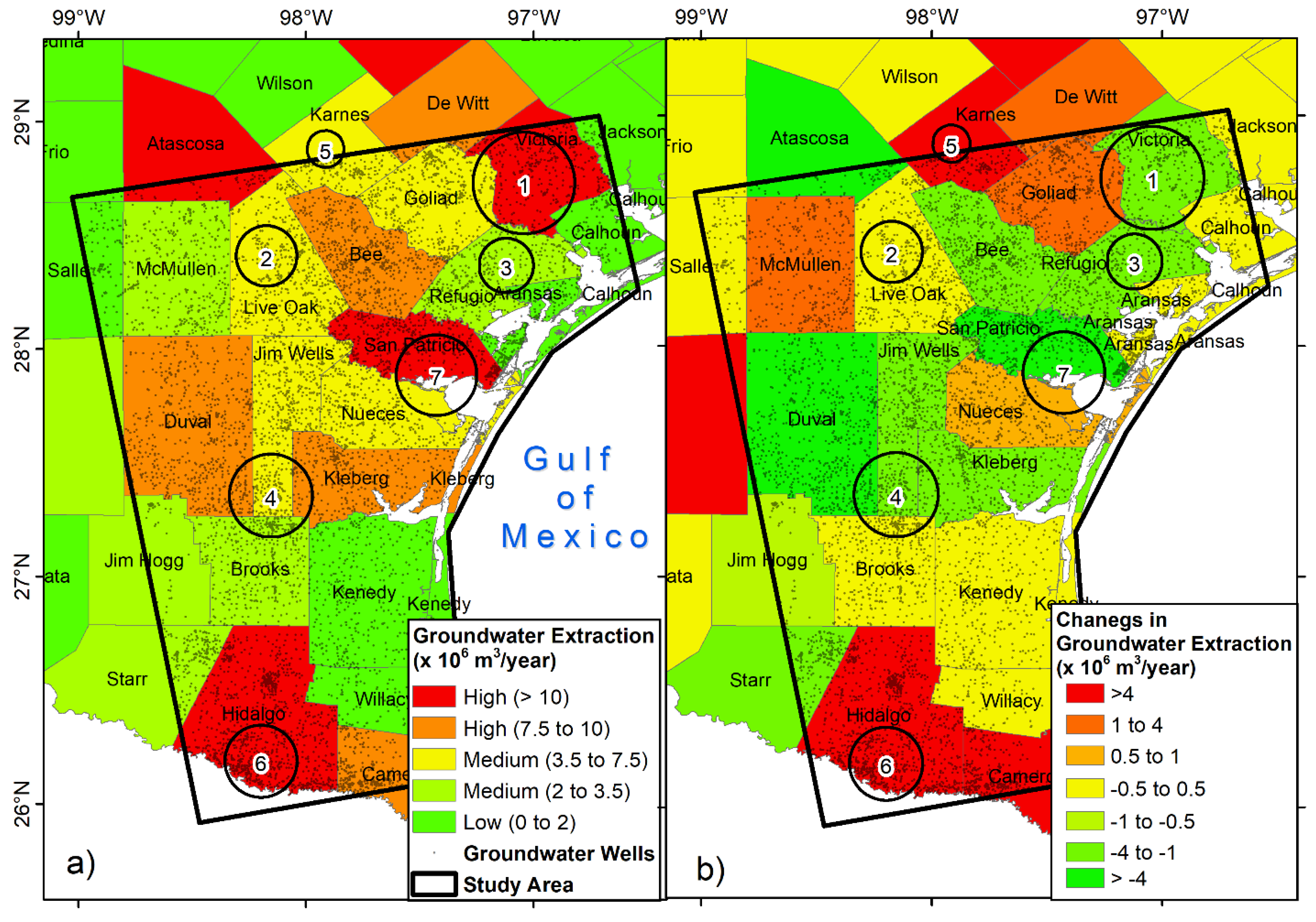
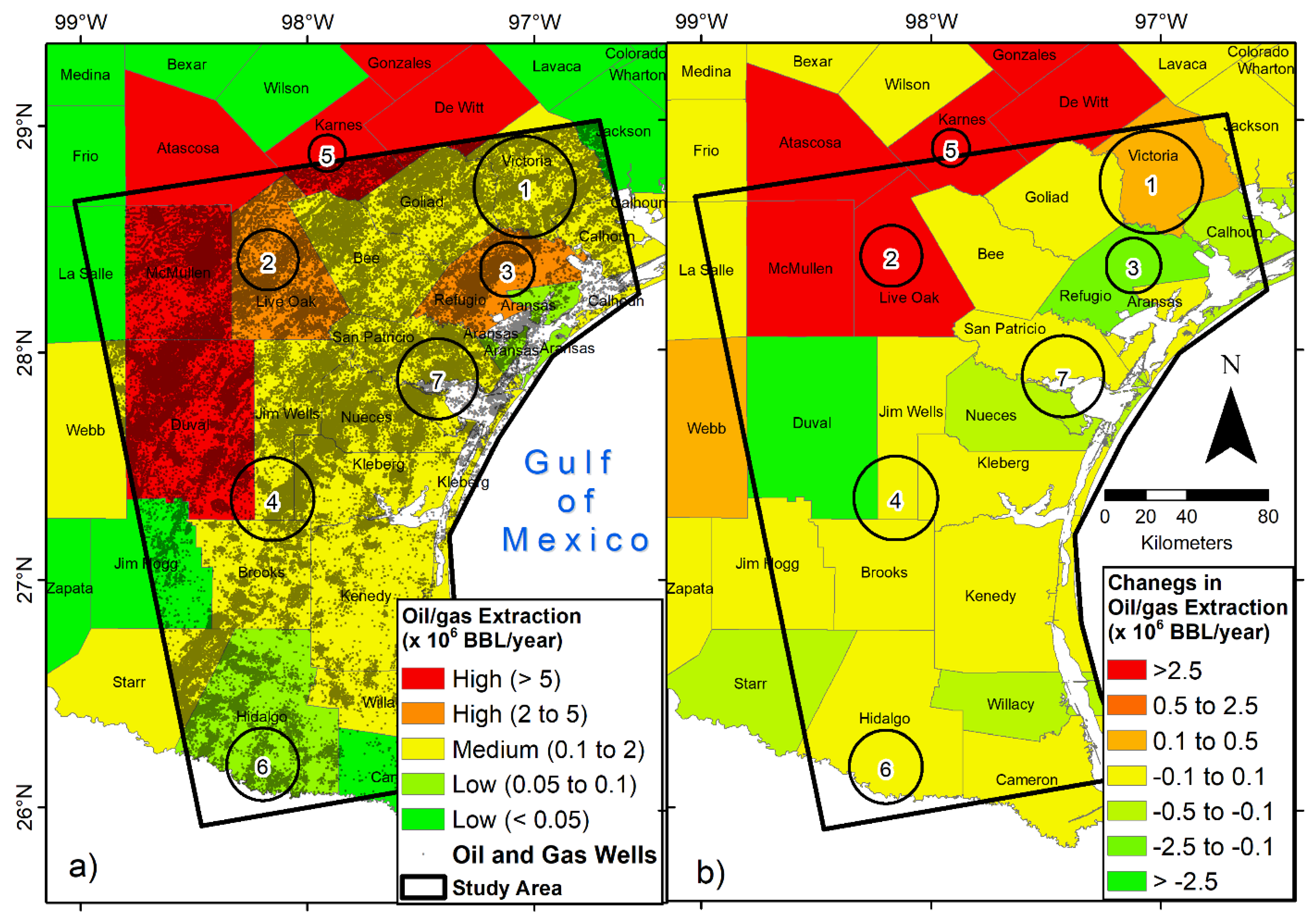
5.2. Factors Controlling Observed Subsidence Rates in the Texas Coastal Bend
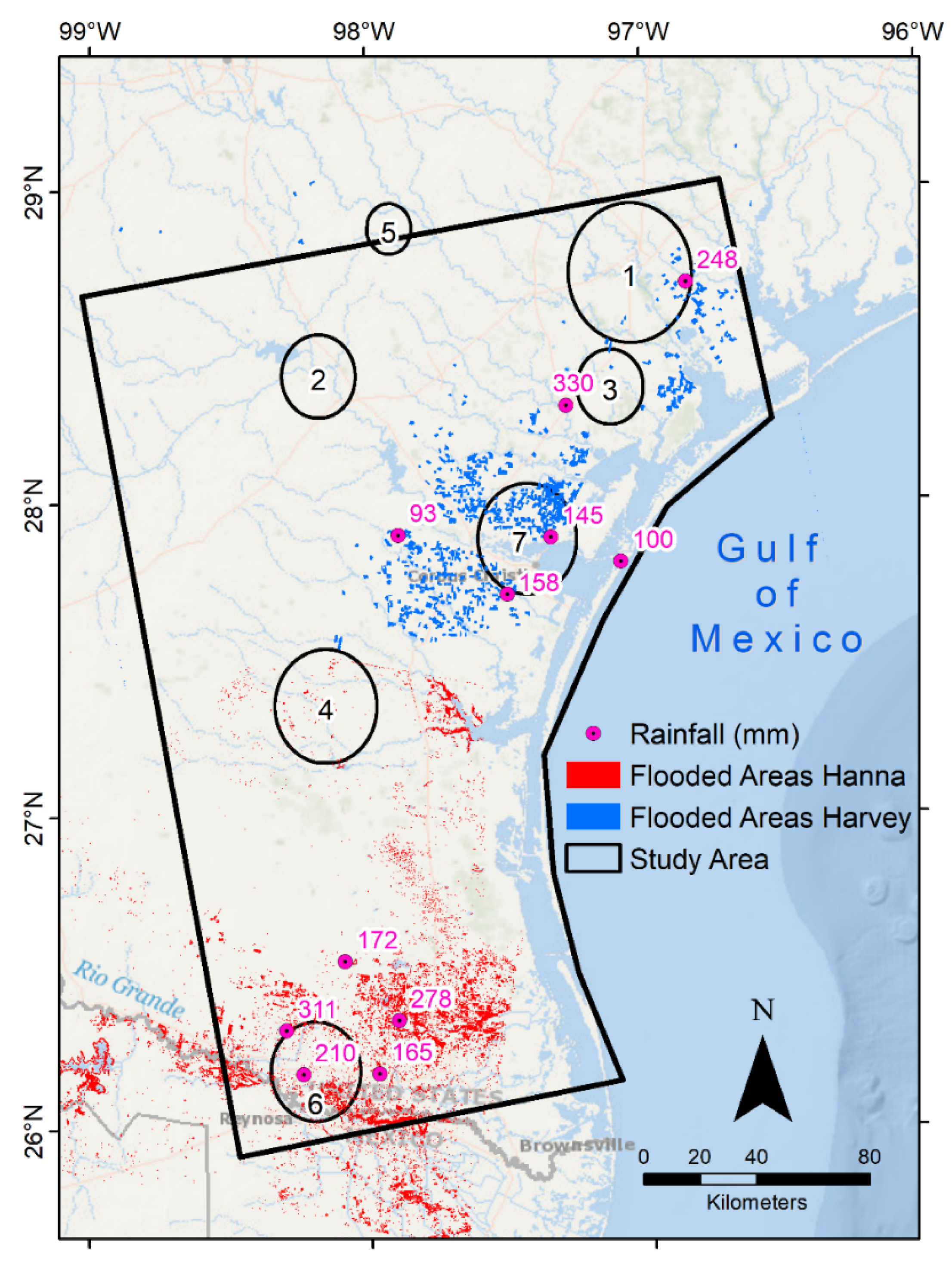
5.3. Consequences of Land Subsidence in the Texas Coastal Bend
6. Discussion
7. Conclusions
Author Contributions
Funding
Institutional Review Board Statement
Informed Consent Statement
Data Availability Statement
Acknowledgments
Conflicts of Interest
Appendix A

| Scene Number | Acquisition Date | Orbit | Spatial Baseline | Temporal Baseline |
|---|---|---|---|---|
| 1 | 24/4/2017 | Ascending | −26 | 0 |
| 2 | 6/5/2017 | Ascending | −116 | 12 |
| 3 | 18/5/2017 | Ascending | −84 | 12 |
| 4 | 30/5/2017 | Ascending | 12 | 12 |
| 5 | 11/6/2017 | Ascending | −10 | 12 |
| 6 | 17/7/2017 | Ascending | −37 | 36 |
| 7 | 29/7/2017 | Ascending | −20 | 12 |
| 8 | 22/8/2017 | Ascending | 50 | 24 |
| 9 | 3/9/2017 | Ascending | 6 | 12 |
| 10 | 15/9/2017 | Ascending | −79 | 12 |
| 11 | 14/11/2017 | Ascending | 11 | 60 |
| 12 | 26/11/2017 | Ascending | −102 | 12 |
| 13 | 8/12/2017 | Ascending | 21 | 12 |
| 14 | 25/1/2018 | Ascending | −53 | 48 |
| 15 | 6/2/2018 | Ascending | −79 | 12 |
| 16 | 18/2/2018 | Ascending | −56 | 12 |
| 17 | 14/3/2018 | Ascending | −5 | 24 |
| 18 | 7/4/2018 | Ascending | 0 | 24 |
| 19 | 1/5/2018 | Ascending | 48 | 24 |
| 20 | 13/5/2018 | Ascending | −57 | 12 |
| 21 | 18/6/2018 | Ascending | −1 | 36 |
| 22 | 12/7/2018 | Ascending | 80 | 24 |
| 23 | 5/8/2018 | Ascending | 11 | 24 |
| 24 | 10/9/2018 | Ascending | 29 | 36 |
| 25 | 16/10/2018 | Ascending | −117 | 36 |
| 26 | 9/11/2018 | Ascending | 48 | 24 |
| 27 | 3/12/2018 | Ascending | −10 | 24 |
| 28 | 8/1/2019 | Ascending | 24 | 36 |
| 29 | 1/2/2019 | Ascending | −24 | 24 |
| 30 | 9/3/2019 | Ascending | −107 | 36 |
| 31 | 2/4/2019 | Ascending | −85 | 24 |
| 32 | 26/4/2019 | Ascending | −140 | 24 |
| 33 | 20/5/2019 | Ascending | −14 | 24 |
| 34 | 13/6/2019 | Ascending | 76 | 24 |
| 35 | 25/6/2019 | Ascending | 0 | 12 |
| Scene Number | Acquisition Date | Orbit | Spatial Baseline | Temporal Baseline |
|---|---|---|---|---|
| 1 | 14/10/2016 | Ascending | 51 | 0 |
| 2 | 25/12/2016 | Ascending | 29 | 72 |
| 3 | 18/1/2017 | Ascending | 24 | 24 |
| 4 | 24/4/2017 | Ascending | 30 | 96 |
| 5 | 6/5/2017 | Ascending | −57 | 12 |
| 6 | 18/5/2017 | Ascending | −27 | 12 |
| 7 | 30/5/2017 | Ascending | 66 | 12 |
| 8 | 29/7/2017 | Ascending | 36 | 60 |
| 9 | 22/8/2017 | Ascending | 104 | 24 |
| 10 | 3/9/2017 | Ascending | 63 | 12 |
| 11 | 15/9/2017 | Ascending | −22 | 12 |
| 12 | 14/11/2017 | Ascending | 62 | 60 |
| 13 | 26/11/2017 | Ascending | −50 | 12 |
| 14 | 8/12/2017 | Ascending | 70 | 12 |
| 15 | 1/1/2018 | Ascending | 155 | 24 |
| 16 | 25/1/2018 | Ascending | 3 | 24 |
| 17 | 18/2/2018 | Ascending | 0 | 24 |
| 18 | 14/3/2018 | Ascending | 47 | 24 |
| 19 | 7/4/2018 | Ascending | 52 | 24 |
| 20 | 13/5/2018 | Ascending | 1 | 36 |
| 21 | 18/6/2018 | Ascending | 55 | 36 |
| 22 | 24/7/2018 | Ascending | 45 | 36 |
| 23 | 17/8/2018 | Ascending | 7 | 24 |
| 24 | 22/9/2018 | Ascending | 66 | 36 |
| 25 | 16/10/2018 | Ascending | −61 | 24 |
| 26 | 9/11/2018 | Ascending | 101 | 24 |
| 27 | 3/12/2018 | Ascending | 41 | 24 |
| 28 | 1/2/2019 | Ascending | 31 | 60 |
| 29 | 9/3/2019 | Ascending | −50 | 36 |
| 30 | 2/4/2019 | Ascending | −28 | 24 |
| 31 | 26/4/2019 | Ascending | −81 | 24 |
| 32 | 20/5/2019 | Ascending | 47 | 24 |
| 33 | 25/6/2019 | Ascending | 56 | 36 |
| Hurricane Harvey | ||
|---|---|---|
| Scene Number | Pre-Event Images | Post-Event Image |
| 1 | 24/4/2017 | 3/9/2017 |
| 2 | 6/5/2017 | |
| 3 | 30/5/2017 | |
| 4 | 11/6/2017 | |
| 5 | 17/7/2017 | |
| 6 | 29/7/2017 | |
| 7 | 22/8/2017 | |
| Hurricane Hanna | ||
| Scene Number | Pre-Event Image | Post-Event Image |
| 1 | 15/7/2020 | 27/7/2020 |
| GNSS Station | T (Years) | Starting Time (Years) | Rate (mm/yr) | 95% CI (mm/yr) |
|---|---|---|---|---|
| txae | 2.74 | 2016.7502 | 0.00 | 1.47 |
| txfe | 10.09 | 2010.5489 | −0.36 | 0.29 |
| txgw | 8.24 | 2012.4052 | −0.49 | 0.37 |
| txbe | 10.08 | 2010.5599 | −1.51 | 0.29 |
| txgo | 10.06 | 2010.5818 | −1.45 | 0.29 |
| txcc | 24.59 | 1996.0548 | −2.01 | 0.09 |
| txvc | 5.33 | 2015.3073 | 0.03 | 0.64 |
| txpo | 9.87 | 2010.7707 | −3.38 | 0.30 |
| txff | 8.24 | 2012.4052 | −5.24 | 0.37 |
| txs5 | 5.65 | 2014.9897 | −1.85 | 0.60 |
| txrv | 7.45 | 2013.1882 | −2.27 | 0.42 |
| txpr | 18.57 | 2002.0753 | −5.72 | 0.13 |
| txpv | 10.33 | 2010.2888 | −1.41 | 0.28 |
References
- Small, C.; Nicholls, R.J. A global analysis of human settlement in coastal zones. J. Coast. Res. 2003, 19, 584–599. [Google Scholar]
- Abidin, H.Z.; Andreas, H.; Gumilar, I.; Sidiq, T.P.; Fukuda, Y. Land subsidence in coastal city of Semarang (Indonesia): Characteristics, impacts and causes. Geomat. Nat. Hazards Risk 2013, 4, 226–240. [Google Scholar] [CrossRef] [Green Version]
- Eggleston, J.; Pope, J. Land Subsidence and Relative Sea-Level Rise in the Southern Chesapeake Bay Region; U.S. Geological Survey: Reston, VA, USA, 2013; ISBN 9781411337169.
- Blackwell, E.; Shirzaei, M.; Ojha, C.; Werth, S. Tracking California’s sinking coast from space: Implications for relative sea-level rise. Sci. Adv. 2020, 6, eaba4551. [Google Scholar] [CrossRef] [PubMed]
- Dolan, A.H.; Walker, I.J. Understanding Vulnerability of Coastal Communities to Climate Change Related Risks. J. Coast. Res. 2006, III, 1316–1323. [Google Scholar]
- Wu, S.Y.; Yarnal, B.; Fisher, A. Vulnerability of coastal communities to sea-level rise: A case study of Cape May County, New Jersey, USA. Clim. Res. 2002, 22, 255–270. [Google Scholar] [CrossRef] [Green Version]
- Felsenstein, D.; Lichter, M. Social and economic vulnerability of coastal communities to sea-level rise and extreme flooding. Nat. Hazards 2014, 71, 463–491. [Google Scholar] [CrossRef]
- Venkataramanan, V.; Packman, A.I.; Peters, D.R.; Lopez, D.; McCuskey, D.J.; McDonald, R.I.; Miller, W.M.; Young, S.L. A systematic review of the human health and social well-being outcomes of green infrastructure for stormwater and flood management. J. Environ. Manag. 2019, 246, 868–880. [Google Scholar] [CrossRef]
- Grineski, S.E.; Flores, A.B.; Collins, T.W.; Chakraborty, J. The impact of Hurricane Harvey on Greater Houston households: Comparing pre-event preparedness with post-event health effects, event exposures, and recovery. Disasters 2019, 44, 408–432. [Google Scholar] [CrossRef]
- Fitzgerald, D.M.; Fenster, M.S.; Argow, B.A.; Buynevich, I.V. Coastal Impacts Due to Sea-Level Rise. Annu. Rev. Warth Planet. Sci. 2008, 36, 601–647. [Google Scholar] [CrossRef] [Green Version]
- Don, N.C.; Hang, N.T.M.; Araki, H.; Yamanishi, H.; Koga, K. Salinization processes in an alluvial coastal lowland plain and effect of sea water level rise. Environ. Geol. 2006, 49, 743–751. [Google Scholar] [CrossRef]
- Bawden, G.W.; Johnson, M.R.; Kasmarek, M.C.; Brandt, J.; Middleton, C.S. Investigation of Land Subsidence in the Houston-Galveston Region of Texas by Using the Global Positioning System and Interferometric Synthetic Aperture Radar, 1993–2000; Scientific Investigations Report No. 2012-5211; U.S. Geological Survey: Reston, VA, USA, 2012; p. 88.
- Liu, Y.; Li, J.; Fasullo, J.; Galloway, D.L. Land subsidence contributions to relative sea level rise at tide gauge Galveston Pier 21, Texas. Sci. Rep. 2020, 10, 17905. [Google Scholar] [CrossRef]
- Davlasheridze, M.; Fan, Q.; Highfield, W.; Liang, J. Economic impacts of storm surge events: Examining state and national ripple effects. Clim. Chang. 2021, 166, 11. [Google Scholar] [CrossRef]
- Khan, S.D.; Huang, Z.; Karacay, A. Study of ground subsidence in northwest Harris county using GPS, LiDAR, and InSAR techniques. Nat. Hazards 2014, 73, 1143–1173. [Google Scholar] [CrossRef]
- Qu, F.; Lu, Z.; Zhang, Q.; Bawden, G.W.; Kim, J.W.; Zhao, C.; Qu, W. Mapping ground deformation over Houston-Galveston, Texas using multi-temporal InSAR. Remote Sens. Environ. 2015, 169, 290–306. [Google Scholar] [CrossRef]
- Zilkoski, D.; Hall, L.; Mitchell, G.; Kammula, V.; Singh, A.; Chrismer, W.; Neighbors, R. The Harris-Galveston Coastal Subsidence District/National Geodetic Survey Automated Global Positioning System Subsidence Monitoring Project. In Proceedings of the US Geological Survey Subsidence Interest Group Conference, Galveston, TX, USA, 27–29 November 2001; Available online: http://fbsubsidence.org/wp-content/uploads/2020/07/GPS-Project.pdf (accessed on 16 November 2021).
- Bourman, R.P.; Murray-Wallace, C.V.; Belperio, A.P.; Harvey, N. Rapid coastal geomorphic change in the River Murray Estuary of Australia. Mar. Geol. 2000, 170, 141–168. [Google Scholar] [CrossRef]
- Zhou, X.; Wang, G.; Wang, K.; Liu, H.; Lyu, H.; Turco, M.J. Rates of Natural Subsidence along the Texas Coast Derived from GPS and Tide Gauge Measurements (1904–2020). J. Surv. Eng. 2021, 147, 04021020. [Google Scholar] [CrossRef]
- Campbell, M.D.; Campbell, D.M.; Wise, H.M.; Bost, R.C. Growth Faulting and Subsidence in the Houston, Texas Area: A Guide to the Origins, Relationships, Hazards, Potential Impacts, and Methods of Investigation; Institute of Environmental Technology: Houston, TX, USA, 2015; 102p. [Google Scholar]
- Verbeek, E.R.; Clanton, U.S. Historically Active Faults in the Houston Metropolitan Area, Texas; Houston Geological Society: Houston, AR, USA, 1981; pp. 28–68. [Google Scholar]
- Becker, M.W. Potential for satellite remote sensing of ground water. Ground Water 2006, 44, 306–318. [Google Scholar] [CrossRef]
- Gambolati, G.; Teatini, P. Geomechanics of subsurface water withdrawal and injection. Water Resour. Res. 2015, 51, 3922–3955. [Google Scholar] [CrossRef]
- Smith, R.; Knight, R. Modeling Land Subsidence Using InSAR and Airborne Electromagnetic Data. Water Resour. Res. 2019, 55, 2801–2819. [Google Scholar] [CrossRef] [Green Version]
- Domenico, P.A.; Schwartz, F.W. Physical and Chemical Hydrogeology, 2nd ed.; John Wiley & Sons: New York, NY, USA, 1997. [Google Scholar]
- Paine, J.G. Subsidence of the Texas coast: Inferences from historical and late Pleistocene sea levels. Tectonophysics 1993, 222, 445–458. [Google Scholar] [CrossRef]
- Gebremichael, E.; Sultan, M.; Becker, R.; El Bastawesy, M.; Cherif, O.; Emil, M. Assessing Land Deformation and Sea Encroachment in the Nile Delta: A Radar Interferometric and Inundation Modeling Approach. J. Geophys. Res. Solid Earth 2018, 123, 3208–3224. [Google Scholar] [CrossRef]
- Hooper, A.; Segall, P.; Zebker, H. Persistent scatterer interferometric synthetic aperture radar for crustal deformation analysis, with application to Volcán Alcedo, Galápagos. J. Geophys. Res. Solid Earth 2007, 112, B07407. [Google Scholar] [CrossRef] [Green Version]
- Ferretti, A.; Fumagalli, A.; Novali, F.; Prati, C.; Rocca, F.; Rucci, A. A New Algorithm for Processing Interferometric Data-Stacks: SqueeSAR. IEEE Trans. Geosci. Remote Sens. 2011, 49, 3460–3470. [Google Scholar] [CrossRef]
- Miller, M.M.; Shirzaei, M.; Argus, D. Aquifer mechanical properties and decelerated compaction in Tucson, Arizona. J. Geophys. Res. Solid Earth 2017, 122, 8402–8416. [Google Scholar] [CrossRef]
- Galloway, D.L.; Burbey, T.J. Review: Regional land subsidence accompanying groundwater extraction. Hydrogeol. J. 2011, 19, 1459–1486. [Google Scholar] [CrossRef]
- Aslan, G.; Lasserre, C.; Cakir, Z.; Ergintav, S.; Özarpaci, S.; Dogan, U.; Bilham, R.; Renard, F. Shallow Creep Along the 1999 Izmit Earthquake Rupture (Turkey) From GPS and High Temporal Resolution Interferometric Synthetic Aperture Radar Data (2011–2017). J. Geophys. Res. Solid Earth 2019, 124, 2218–2236. [Google Scholar] [CrossRef]
- Blachowski, J.; Kopec, A.; Milczarek, W.; Owczarz, K. Evolution of secondary deformations captured by satellite radar interferometry: Case study of an abandoned coal basin in SW Poland. Sustainability 2019, 11, 884. [Google Scholar] [CrossRef] [Green Version]
- Othman, A.; Sultan, M.; Becker, R.; Alsefry, S.; Alharbi, T.; Gebremichael, E.; Alharbi, H.; Abdelmohsen, K. Use of Geophysical and Remote Sensing Data for Assessment of Aquifer Depletion and Related Land Deformation. Surv. Geophys. 2018, 39, 543–566. [Google Scholar] [CrossRef] [Green Version]
- Galloway, D.L.; Hudnut, K.W.; Ingebritsen, S.E.; Phillips, S.P.; Peltzer, G.; Rogez, F.; Rosen, P.A. Detection of aquifer system compaction and land subsidence using interferometric synthetic aperture radar, Antelope Valley, Mojave Desert, California. Water Resour. Res. 1998, 34, 2573–2585. [Google Scholar] [CrossRef]
- Hu, X.; Bürgmann, R.; Lu, Z.; Handwerger, A.L.; Wang, T.; Miao, R. Mobility, Thickness, and Hydraulic Diffusivity of the Slow-Moving Monroe Landslide in California Revealed by L-Band Satellite Radar Interferometry. J. Geophys. Res. Solid Earth 2019, 124, 7504–7518. [Google Scholar] [CrossRef] [Green Version]
- Chini, M.; Pelich, R.; Pulvirenti, L.; Pierdicca, N.; Hostache, R.; Matgen, P. Sentinel-1 InSAR coherence to detect floodwater in urban areas: Houston and hurricane harvey as a test case. Remote Sens. 2019, 11, 107. [Google Scholar] [CrossRef] [Green Version]
- Miller, M.M.; Shirzaei, M. Land subsidence in Houston correlated with flooding from Hurricane Harvey. Remote Sens. Environ. 2019, 225, 368–378. [Google Scholar] [CrossRef]
- Stukey, J.; Narasimhan, B.; Srinivasan, R. Corpus Christi Bay, Galveston Bay, Mission-Aransas Bay, San Antonio Bay, and Sabine Lake Lower-Watershed Multi-year Land-Use and Land Cover Classifications and Curve Numbers TWDB Contract # 0804830788; Spatial Sciences Lab, Department of Ecosystem Science and Management, and Texas A & M University: College Station, TX, USA, 2004. [Google Scholar]
- Stoeser, D.B.; Shock, N.; Green, G.N.; Dumonceaux, G.M.; Heran, W.D. Geologic Map Database of Texas; U.S. Geological Survey: Reston, VA, USA, 2005.
- Baker, E.T.J. Stratigraphic Nomenclature and Geologic Sections of the Gulf; U.S. Geological Survey Open-File Report 94-461; U.S. Geological Survey: Reston, VA, USA, 1995; p. 34.
- Ryder, P.D.; Ardis, A.F. Hydrology of the Texas Gulf Coast Aquifer Systems; U.S. Geological Survey Professional Paper; U.S. Geological Survey: Reston, VA, USA, 2002.
- Bruun, B.; Jackson, K.; Lake, P.; Walker, J. Texas Aquifers Study Groundwater Quantity, Quality, Flow, and Contributions to Surface Water. 2016. Available online: https://www.twdb.texas.gov/groundwater/docs/studies/TexasAquifersStudy_2016.pdf (accessed on 16 November 2021).
- Jackson, M.P.A.; Roberts, D.G.; Snelson, S. Cenozoic Structural Evolution and Tectono-Stratigraphic Framework of the Northern Gulf Coast Continental Margin. Salt Tecton. 2020, 65, 109–151. [Google Scholar] [CrossRef]
- Chowdhury, A.H.; Mace, R.E. Chapter 10 Groundwater Models of the Gulf Coast Aquifer of Texas. 2001; pp. 173–204. Available online: https://www.twdb.texas.gov/publications/reports/numbered_reports/doc/R365/ch10-GulfCoastModelingPaper.pdf (accessed on 16 November 2021).
- Chowdhury, A.H.; Wade, S.; Mace, R.E.; Ridgeway, C. Groundwater Availability Model of the Central Gulf Coast Aquifer System: Numerical Simulations through 1999. Tex. Water Dev. Board 2004, 1, 14. [Google Scholar]
- Kim, J.W.; Lu, Z. Association between localized geohazards in West Texas and human activities, recognized by Sentinel-1A/B satellite radar imagery. Sci. Rep. 2018, 8, 4727. [Google Scholar] [CrossRef]
- ESA. ESA’s Radar Observatory Mission for GMES Operational Services; ESA: Paris, France, 2012; Volume 1, ISBN 9789292214180. [Google Scholar]
- Emil, M.K.; Sultan, M.; Alakhras, K.; Sataer, G.; Gozi, S.; Al-Marri, M.; Gebremichael, E. Countrywide Monitoring of Ground Deformation Using InSAR Time Series: A Case Study from Qatar. Remote Sens. 2021, 13, 702. [Google Scholar] [CrossRef]
- Blewitt, G.; Hammond, W.; Kreemer, C. Harnessing the GPS Data Explosion for Interdisciplinary Science. Eos 2018, 99, 485. [Google Scholar] [CrossRef]
- Blewitt, G.; Kreemer, C.; Hammond, W.C.; Gazeaux, J. MIDAS robust trend estimator for accurate GPS station velocities without step detection. J. Geophys. Res. Solid Earth 2016, 121, 2054–2068. [Google Scholar] [CrossRef]
- Altamimi, Z.; Rebischung, P.; Métivier, L.; Collilieux, X. ITRF2014: A new release of the International Terrestrial Reference Frame modeling nonlinear station motions. J. Geophys. Res. Solid Earth 2016, 121, 6109–6131. [Google Scholar] [CrossRef] [Green Version]
- Wang, G.; Asce, M. The 95% Confidence Interval for GNSS-Derived Site Velocities. J. Surv. Eng. 2021, 148, 04021030. [Google Scholar] [CrossRef]
- Gebremichael, E.; Molthan, A.L.; Bell, J.R.; Schultz, L.A.; Hain, C. Flood hazard and risk assessment of extreme weather events using synthetic aperture radar and auxiliary data: A case study. Remote Sens. 2020, 12, 3588. [Google Scholar] [CrossRef]
- Zhang, M.; Chen, F.; Liang, D.; Tian, B.; Yang, A. Use of sentinel-1 grd sar images to delineate flood extent in Pakistan. Sustainbility 2020, 12, 5784. [Google Scholar] [CrossRef]
- Inglacla, J.; Mercier, G. A new statistical similarity measure for change detection in multitemporal SAR images and its extension to multiscale change analysis. IEEE Trans. Geosci. Remote Sens. 2007, 45, 1432–1445. [Google Scholar] [CrossRef] [Green Version]
- Ewing, T.E.; Anderson, R.; Babalola, O.; Hubby, K.; Padilla y Sanchez, R.; Reed, R. Structural Syles of the Wilcox and Frio Growth-Fault Trends in Texas: Constraints on Geopressured Resevoirs; University of Texas: Austin, TX, USA, 1987. [Google Scholar]
- Hammes, U.; Loucks, R.G.; Brown, L.F.; Treviño, R.H.; Remington, R.L.; Montoya, P. Structural Setting and Sequence Architecture of a Growth-Faulted. Corpus 2004, 54, 237–246. [Google Scholar]
- Young, S.C.; Knox, P.R.; Baker, E.; Budge, T.; Galloway, B.; Kalbouss, R.; Deeds, N.; Station, C. Final Hydrostratigraphy of the Gulf Coast Aquifer from the Brazos River to the Rio Grande; Texas Water Development Board: Austin, TX, USA, 2010; pp. 1–213.
- Young, S.C.; Ewing, T.; Hamlin, S.; Baker, E.; Lupton, D. Final Report Updating the Hydrogeologic Framework for the Northern Portion of the Gulf Coast Aquifer; Texas Water Development Board: Austin, TX, USA, 2012; p. 283.
- Ferretti, A.; Prati, C.; Rocca, F. Permanent Scatterers in SAR Interferometry. IEEE Trans. Geosci. Remote Sens. 2001, 39, 8–20. [Google Scholar] [CrossRef]
- Hooper, A.; Zebker, H.; Segall, P.; Kampes, B. A new method for measuring deformation on volcanoes and other natural terrains using InSAR persistent scatterers. Geophys. Res. Lett. 2004, 31, L23611. [Google Scholar] [CrossRef]
- Ferretti, A.; Monti-Guarnieri, A.; Prati, C.; Rocca, F.; Massonnet, D. InSAR Principles-Guidelines for SAR Interferometry Processing and Interpretation; Fletcher, K., Ed.; European Space Agency: Noordwijk, The Netherland, 2007; ISBN 9290922338. [Google Scholar]
- Hanssen, R.F. Radar Interferometry: Data Interpretation and Error Analysis; Springer: New York, NY, USA, 2001; Volume 328, ISBN 978-0-306-47633-4. [Google Scholar]
- Foumelis, M.; Blasco, J.M.D.; Desnos, Y.L.; Engdahl, M.; Fernández, D.; Veci, L.; Lu, J.; Wong, C. ESA SNAP—Stamps integrated processing for Sentinel-1 persistent scatterer interferometry. In Proceedings of the IGARSS 2018—2018 IEEE International Geoscience and Remote Sensing Symposium, Valencia, Spain, 22–27 July 2018; pp. 1364–1367. [Google Scholar] [CrossRef]
- Hooper, A.; Spaans, K.; Bekaert, D.; Cuenca, M.C.; Arıkan, M. StaMPS/MTI Manual; Delft University of Technology: Delft, The Netherlands, 2010. [Google Scholar]
- Yu, C.; Penna, N.T.; Li, Z. Generation of real-time mode high-resolution water vapor fields from GPS observations. J. Geophys. Res. 2017, 122, 2008–2025. [Google Scholar] [CrossRef]
- Yu, C.; Li, Z.; Penna, N.T. Interferometric synthetic aperture radar atmospheric correction using a GPS-based iterative tropospheric decomposition model. Remote Sens. Environ. 2018, 204, 109–121. [Google Scholar] [CrossRef]
- Yu, C.; Li, Z.; Penna, N.T.; Crippa, P. Generic Atmospheric Correction Model for Interferometric Synthetic Aperture Radar Observations. J. Geophys. Res. Solid Earth 2018, 123, 9202–9222. [Google Scholar] [CrossRef]
- Bahr, T.; Europe, S.E. Sarscape Analytics Toolbox. 2020. Available online: https://www.sarmap.ch/index.php/2020/07/10/sarscape-last-version/ (accessed on 16 November 2021).
- Bekaert, D.P.S.; Hamlington, B.D.; Buzzanga, B.; Jones, C.E. Spaceborne Synthetic Aperture Radar Survey of Subsidence in Hampton Roads, Virginia (USA). Sci. Rep. 2017, 7, 14752. [Google Scholar] [CrossRef] [PubMed] [Green Version]
- Liu, Y.; Zhao, C.; Zhang, Q.; Lu, Z.; Zhang, J. A constrained small baseline subsets (CSBAS) InSAR technique for multiple subsets. Eur. J. Remote. Sens. 2019, 53, 14–26. [Google Scholar] [CrossRef] [Green Version]
- Gourmelen, N.; Amelung, F.; Lanari, R. Interferometric synthetic aperture radar–GPS integration: Interseismic strain accumulation across the Hunter Mountain fault in the eastern California shear zone. J. Geophys. Res. Solid Earth 2010, 115, B09408. [Google Scholar] [CrossRef] [Green Version]
- Jiang, J.; Lohman, R.B. Coherence-guided InSAR deformation analysis in the presence of ongoing land surface changes in the Imperial Valley, California. Remote Sens. Environ. 2021, 253, 112160. [Google Scholar] [CrossRef]
- Emanuel, K. Assessing the present and future probability of Hurricane Harvey’s rainfall. Proc. Natl. Acad. Sci. USA 2017, 114, 12681–12684. [Google Scholar] [CrossRef] [Green Version]
- Brown, D.P.; Berge, R.; Brad, R. National Hurricane Center Tropical Cyclone Report. Hurricane Hanna; National Hurricane Center: Miami, FL, USA, 2020; pp. 1–49.
- Hooper, A.J. A multi-temporal InSAR method incorporating both persistent scatterer and small baseline approaches. Geophys. Res. Lett. 2008, 35, L16302. [Google Scholar] [CrossRef] [Green Version]


| SAR Instrument | Orbit Type | Track | Frame | No. of Images | Perpendicular Baseline | Temporal Baseline | ||
|---|---|---|---|---|---|---|---|---|
| Mean | Max | Mean | Max | |||||
| Sentinel-1 | Ascending | 107 | 83 | 35 | 48 | 140 | 32 | 60 |
| Sentinel-1 | Ascending | 107 | 88 | 33 | 45 | 147 | 24 | 60 |
| Event | SAR Instrument | Orbit Type | Track | Frame | Pre-Event Images | Post-Event Images |
|---|---|---|---|---|---|---|
| Harvey | Sentinel-1 | Ascending | 107 | 88 | 7 | 1 |
| Hanna | Sentinel-1 | Descending | 41 | 503 | 1 | 1 |
| Polygon/Region | PS Points (count) | Minimum Displacement (mm/yr) | Maximum Displacement (mm/yr) | Average Displacement (mm/yr) | Standard Deviation (mm/yr) |
|---|---|---|---|---|---|
| 1 | 8111 | −27.48 | 7.19 | −7.55 | 3.45 |
| 2 | 1016 | −14.77 | −0.37 | −9.02 | 2.10 |
| 3 | 254 | −15.31 | 3.59 | −8.67 | 2.90 |
| 4 | 807 | −21.25 | 2.85 | −9.48 | 3.74 |
| 5 | 731 | −24.13 | 14.76 | −5.24 | 5.62 |
| 6 | 22159 | −13.04 | 9.66 | −2.64 | 2.75 |
| 7 | 7381 | −16.02 | 7.68 | −3.53 | 2.33 |
Publisher’s Note: MDPI stays neutral with regard to jurisdictional claims in published maps and institutional affiliations. |
© 2022 by the authors. Licensee MDPI, Basel, Switzerland. This article is an open access article distributed under the terms and conditions of the Creative Commons Attribution (CC BY) license (https://creativecommons.org/licenses/by/4.0/).
Share and Cite
Haley, M.; Ahmed, M.; Gebremichael, E.; Murgulet, D.; Starek, M. Land Subsidence in the Texas Coastal Bend: Locations, Rates, Triggers, and Consequences. Remote Sens. 2022, 14, 192. https://doi.org/10.3390/rs14010192
Haley M, Ahmed M, Gebremichael E, Murgulet D, Starek M. Land Subsidence in the Texas Coastal Bend: Locations, Rates, Triggers, and Consequences. Remote Sensing. 2022; 14(1):192. https://doi.org/10.3390/rs14010192
Chicago/Turabian StyleHaley, Michael, Mohamed Ahmed, Esayas Gebremichael, Dorina Murgulet, and Michael Starek. 2022. "Land Subsidence in the Texas Coastal Bend: Locations, Rates, Triggers, and Consequences" Remote Sensing 14, no. 1: 192. https://doi.org/10.3390/rs14010192
APA StyleHaley, M., Ahmed, M., Gebremichael, E., Murgulet, D., & Starek, M. (2022). Land Subsidence in the Texas Coastal Bend: Locations, Rates, Triggers, and Consequences. Remote Sensing, 14(1), 192. https://doi.org/10.3390/rs14010192