BiFDANet: Unsupervised Bidirectional Domain Adaptation for Semantic Segmentation of Remote Sensing Images

Abstract

When segmenting massive amounts of remote sensing images collected from different satellites or geographic locations (cities), the pre-trained deep learning models cannot always output satisfactory predictions. To deal with this issue, domain adaptation has been widely utilized to enhance the generalization abilities of the segmentation models. Most of the existing domain adaptation methods, which based on image-to-image translation, firstly transfer the source images to the pseudo-target images, adapt the classifier from the source domain to the target domain. However, these unidirectional methods suffer from the following two limitations: (1) they do not consider the inverse procedure and they cannot fully take advantage of the information from the other domain, which is also beneficial, as confirmed by our experiments; (2) these methods may fail in the cases where transferring the source images to the pseudo-target images is difficult. In this paper, in order to solve these problems, we propose a novel framework BiFDANet for unsupervised bidirectional domain adaptation in the semantic segmentation of remote sensing images. It optimizes the segmentation models in two opposite directions. In the source-to-target direction, BiFDANet learns to transfer the source images to the pseudo-target images and adapts the classifier to the target domain. In the opposite direction, BiFDANet transfers the target images to the pseudo-source images and optimizes the source classifier. At test stage, we make the best of the source classifier and the target classifier, which complement each other with a simple linear combination method, further improving the performance of our BiFDANet. Furthermore, we propose a new bidirectional semantic consistency loss for our BiFDANet to maintain the semantic consistency during the bidirectional image-to-image translation process. The experiments on two datasets including satellite images and aerial images demonstrate the superiority of our method against existing unidirectional methods.

1. Introduction

In the last few years, it has been possible to collect a mass of remote sensing images, thanks to the continuous advancement of remote sensing techniques. For example, Gaofen satellites can capture a large number of satellite images with high spatial resolution on a large scale. In remote sensing, such a large amount of data has offered many more capability for image analysis tasks; for example, semantic segmentation [1], change detection [2] and scene classification [3]. Among these tasks, the semantic segmentation of remote sensing images has become one of the most interesting and important research topics because it is widely used in many applications, such as dense labeling, city planning, urban management, environment monitoring, and so on.

For the semantic segmentation of remote sensing images, CNN [4] has become one of the most efficient methods in the past decades and several CNN models have shown their effectiveness, such as DeepLab [5] and its variants [6,7]. However, these methods have some limitations, because CNN-based architectures tend to be sensitive to the distributions and features of the training images and test images. Even though they give satisfactory predictions when the distributions of training and test images are similar [1], when we attempt to use this model to classify images obtained from other satellites or cities, the classification accuracy severely decreases due to different distributions of the source images and target images, as shown in Figure 1. In the literature, the aforementioned problem is known as domain adaptation [8]. In remote sensing, domain gap problems are often caused due to many reasons, such as illumination conditions, imaging times, imaging sensors, geographic locations and so on. These factors will change the spectral characteristics of objects and resulted in a large intra-class variability. For instance, the images acquired from different satellite sensors may have different colors, as shown in Figure 1a,b. Similarly, due to the differences of the imaging sensors, images may have different types of channels. For example, a few images may consist of near-infrared, green, and red channels while the others may have green, red, and blue bands.

In typical domain adaptation problems, the distributions of the source domain are different from those of the target domain. In remote sensing, we assume that the images collected from different satellites or locations (cities) are different domains. The unsupervised domain adaptation defines that only annotations of the source domain are available and aims at generating satisfactory predicted labels for the unlabeled target domain, even if the domain shift between the source domain and target domain is huge. To improve the performances of the segmentation models in aforementioned settings, one of the most common approaches in remote sensing is to diversify the training images of the source domain, by performing data augmentation techniques, such as random color change [9], histogram equalization [10], and gamma correction [11]. However, even if these methods slightly increase the generalization capabilities of the models, the improvement is unsatisfactory when there exists huge differences between the distributions of different domains. For example, it is difficult to adapt the classifier from one domain with near-infrared, red, and green bands to another one with red, green and blue channels by using simple data augmentation techniques. To overcome such limitation, a generative adversarial network [12] was applied to transfer images between the source and target domains and made significant progress in unsupervised domain adaptation for semantic segmentation [13,14]. These approaches based on image translation can be divided into two steps. At first, it learns to transfer the source images to the target domain. Secondly, the translated images and the labels for the corresponding source images are used to train the classifier which will be tested on the unlabeled source domain. When the first step reduce the domain shift, the second step can effectively adapt the segmentation model to the target domain. In addition, inverse translations which adapt the segmentation model from the target domain to the source domain have been implemented as well [15]. In our experiments, we find that these two translations in opposite directions should be complementary rather than alternative. Furthermore, such unidirectional (e.g., source-to-target) setting might ignore the information from the inverse direction. For example, Benjdira et al. [16] adapted the source classifier to the unlabeled target domain, they only simulated the distributions of the target images instead of making the target images fully participate in domain adaption. Therefore, these unidirectional methods cannot take full advantage of the information from the target domain. Meanwhile, the key to the domain adaptation methods based on image translation is the similarity between the distributions of the pseudo-target images and the target images. Given fixed image translation models, it will depend on the difficulty of converting between two domains: there might be some situations where transferring the target images to the source domain is more difficult, and situations where transferring the source images to the target domain is more difficult. By combining the two opposite directions, we will acquire an architecture more general than those unidirectional methods. Furthermore, the recent image translation network (e.g., CycleGAN [17]) is bidirectional so that we can usually obtain two image generators in the source-to-target and target-to-source directions when the training of the image translation model is done. We can use both of generators to make the best of the information from the two directions.

However, solving the aforementioned problems presents a few challenges. First, the transformed images and their corresponding original images must have the same semantic contents with the original images. For instance, if the image-to-image translation model replaces buildings with bare land during the translation, the labels of the original images cannot match the transformed images. As a result, semantic changes in any directions will affect our models. If the semantic changes occur in the source-to-target direction, the target domain classifier will have poor performance. If the approach replaces some objects with others in the target-to-source direction, the predicted labels of the source domain classifier would be unsatisfactory. Secondly, when we transfer the source images to the target domain, the data distributions of the pseudo-target images should be as similar as possible to the data distributions of the target images and the data distributions of the pseudo-source and source images should be similar as well. Otherwise, the transformed images of one domain cannot represent the other domain. Finally, the predicted labels of the two directions complement each other and the method of combining the labels is crucial because it will affect the final predicted labels. Simply combining the two predicted labels may leave out some correct objects or add some wrong objects.

In this article, we propose a new bidirectional model to address the above challenges. This framework involves two opposite directions. In the source-to-target direction, we generate pseudo-target transformed images which are semantically consistent with the original images. For this purpose, we propose a bidirectional semantic consistency loss to maintain the semantic consistency during the image translation. Then we employ the labels of the source images and their corresponding transformed images to adapt the segmentation model to the target domain. In the target-to-source direction, we optimize the source domain classifier to predict labels for the pseudo-source transformed images. These two classifiers may make different types of mistakes and assign different confidence ranks to the predicted labels. Overall the two classifiers are complementary instead of alternative. We make full use of them with a simple linear method which fuses their probability output.

Our contributions are as follows:

(1)

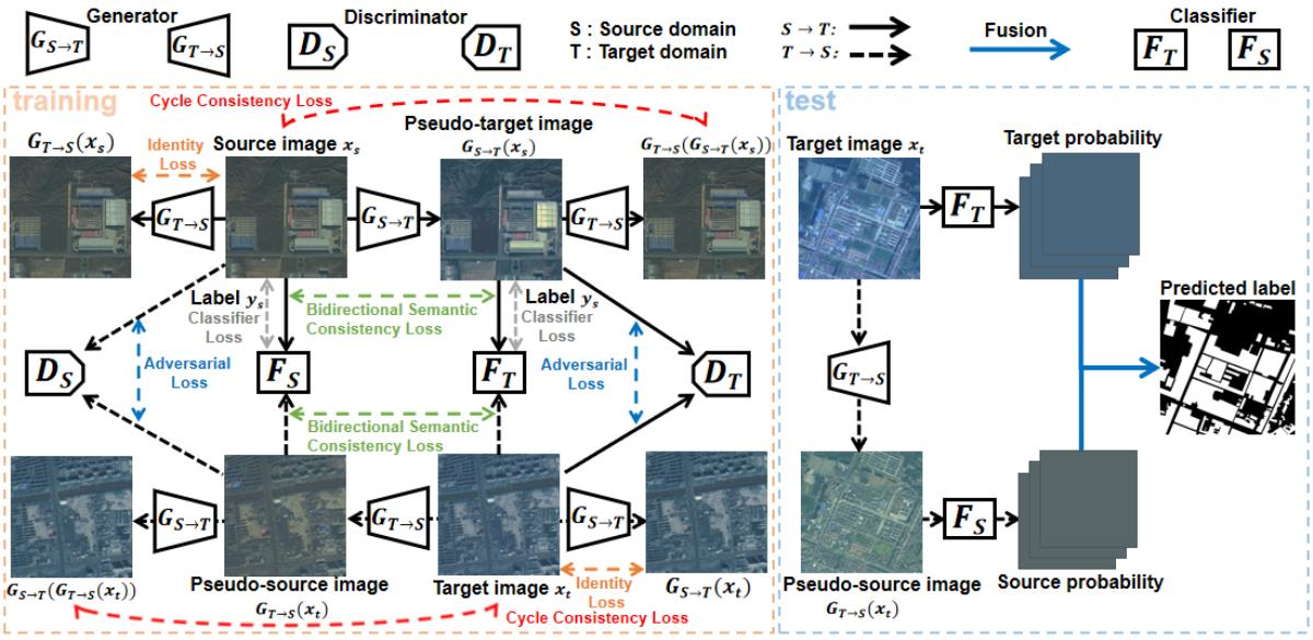
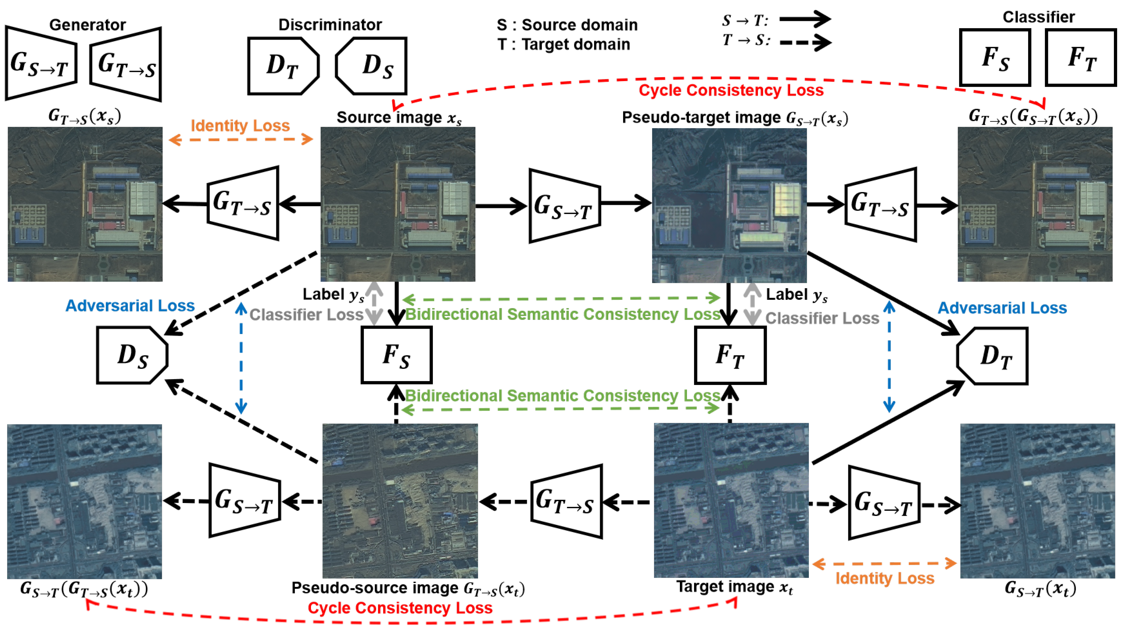
We propose a new unsupervised bidirectional domain adaptation method, coined BiFDANet, for semantic segmentation of remote sensing images, which conducts bidirectional image translation to minimize the domain shift and optimizes the classifiers in two opposite directions to take full advantage of the information from both domains. At test stage, we employ a linear combination method to take full advantage of the two complementary predicted labels which further enhances the performance of our BiFDANet. As far as we know, BiFDANet is the first work on unsupervised bidirectional domain adaptation for semantic segmentation of remote sensing images.

(2)

We propose a new bidirectional semantic consistency loss which effectively supervises the generators to maintain the semantic consistency in both source-to-target and target-to-source directions. We analyze the bidirectional semantic consistency loss by comparing it with two semantic consistency losses used in the existing approaches.

(3)

We perform our proposed framework on two datasets, one consisting of satellite images from two different satellites and the other is composed of aerial images from different cities. The results indicate that our method can improve the performance of the cross-domain semantic segmentation and minimize the domain gap effectively. In addition, the effect of each component is discussed.

This article is organized as follows: Section 2 summarizes the related works. Section 3 presents the theory of our proposed framework. Section 4 describes the data set, the experimental design and discusses the obtained results, Section 5 provides the discussion and Section 6 draws our conclusions.

2. Related Work

2.1. Domain Adaptation

Tuia et al. [8] explained that in the research literature the adaptation methods could be grouped as: the selection of invariant features [18,19,20,21], the adaptation of classifiers [22,23,24,25,26,27], the adaptation of the data distributions [28,29,30,31] and active learning [32,33,34]. Here we focus on the methods of aligning the data distributions by performing image-to-image translation [35,36,37,38,39] between the different domains [40,41,42,43]. These methods usually match the data distributions of different domains by transferring the images from the source domain to the target domain. Next, the segmentation model is trained on the transferred images to classify the target images. In the fields of computer vision, Gatys et al. [40] raised a style transfer method to synthesizes fake images by combining the source contents with the target style. Similarly, Shrivastava et al. [41] generated realistic samples from synthetic images and the synthesized images could train a classification model on real images. Bousmalis et al. [42] learned the source-to-target transformation in the pixel space and transformed source images to target-like images. Taigman et al. [44] proposed a compound loss function to enforce the image generation network to transfer images from target to themselves. Hoffman et al. [14] used CycleGAN [17] to transfer the source images into the target style alternatively and transformed images were input into the classifier to improve its performance in the target domain. Zhao et al. [45] transformed fake images to the target domain which performed pixel-level and feature-level alignments with sub-domain aggregation. The segmentation model trained on such transformed images with the style of the target domain outperformed several unsupervised domain adaptation approaches. In remote sensing, Graph matching [46] and histogram matching [47] were employed to perform abovementioned image-to-image translation. Benjdira et al. [16] generated the fake target-like images by using CycleGAN [17], then the target-like images are used to adapt the source classifier to segment the target images. Similarly, Tasar et al. proposed ColorMapGAN [48], SemI2I [49] and DAugNet [50] to perform image-to-image translation between satellite image pairs to reduces the impact of domain gap. All the above mentioned methods focus on adapting the source segmentation model to the target domain without taking into account the opposite target-to-source direction that is beneficial.

2.2. Bidirectional Learning

Bidirectional learning was used to approach the neural machine translation problem [51,52], which train a language translation system in opposite directions of a language pair. Compared with unidirectional learning, it can improve the performance of the model effectively. Recently, bidirectional learning was applied to image-to-image translation problems as well. Li et al. [53] learned the image translation model and the segmentation adaptation model alternatively with a bidirectional learning method. Chen et al. [54] presented a bidirectional cross-modality adaptation method that aligned different domains from feature and image perspectives. Zhang et al. [55] adapted the model by minimizing the pixel-level and feature-level gaps. The theses method does not optimize the segmentation model in the target-to-source directions. Yang et al. [56] proposed a bi-directional generation network that trained a simple framework for image translation and classification from source to target and from target to source. Jiang et al. [57] proposed a bidirectional adversarial training method which performs adversarial trainings with generating adversarial examples from source to target and back. These methods only use bidirectional learning techniques in training process, but at test time, they do not make full use of two domains even if they have optimized the classifiers in both directions. Russo et al. [58] proposed a bidirectional image translation approach which trained two classifiers on different domains respectively and finally fuses the classification results. However, semantic segmentation task is more sensitive to pixel category while classification task focuses on image category. This proposed method can only be used to deal with the classification tasks, which can’t apply to semantic segmentation tasks directly because it may not preserve the semantic contents.

3. Materials and Methods

The unsupervised domain adaptation assumes that the labeled source domain ($X_S$,$Y_S$) and unlabeled target domain $X_T$ are available. The goal is to train a framework which correctly predicts the results for unlabeled target domain $X_T$.

The proposed BiFDANet consists of bidirectional image translation and bidirectional segmentation adaptation. It learns to transfer source images to the target domain and transfer target images to the source domain, and then optimizes the source classifier $F_S$ and the target classifier $F_T$ in two opposite directions. In this section, we detail how we transfer images between the source and target domain. And then we introduce how we adapt the classifier $F_T$ to the target domain and optimize the classifier $F_S$ in the target-to-source direction. Thereafter, we describe how we combine the two predicted results of the two classifiers $F_S$ and $F_T$. Finally, we illustrate the implementations of the network architectures.

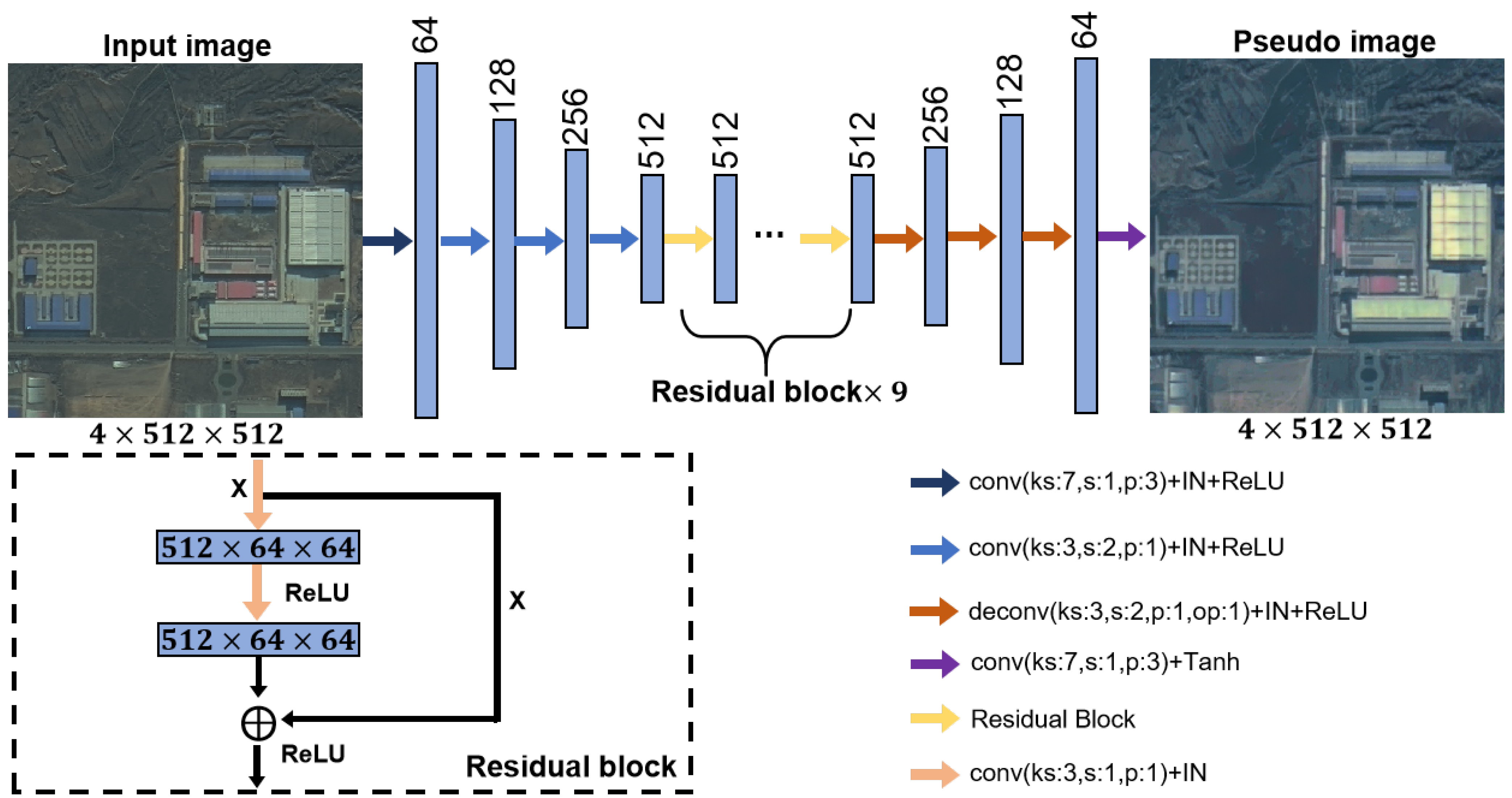
3.1. Bidirectional Image Translation

To perform bidirectional image translation between different domains, we use two generators and two discriminators based on GAN [12] architecture and we add two classifiers to extract the contents from the images. $G_{S\to T}$ denotes the target generator which generates pseudo-target images, $G_{T\to S}$ denotes the source generator which generates pseudo-source images. $D_S$, $D_T$ denote the discriminators and $F_S$, $F_T$ are the classifiers.

First of all, we want the source images $x_s$ and the pseudo-source images $G_{T\to S}\left(x_t\right)$ to be drawn form similar data distributions, while the target images $x_t$ and the pseudo-target images $G_{S\to T}\left(x_s\right)$ have similar data distributions. To deal with these issues, we enforce the data distributions of the pseudo-target images $G_{S\to T}\left(x_s\right)$ and the pseudo-source images $G_{T\to S}\left(x_t\right)$ to be similar to that of the target domain and the source domain respectively by applying adversarial learning (see Figure 2 blue portion). The discriminator $D_S$ discriminates between the source images and the pseudo-source images while the discriminator $D_T$ distinguishes the pseudo-target images from the target domain. We train the generators to fool the discriminators while the discriminators $D_T$ and $D_S$ attempt to classify the images from the target domain and the source domain. The adversarial loss for the target generator $G_{S\to T}$ and the discriminator $D_T$ in the source-to-target direction is as follows:

$${\mathcal{L}}_{adv}^{S\to T}(D_T,G_{S\to T})={\mathbb{E}}_{x_t\sim X_T}[log{D}_T\left(x_t\right)]+{\mathbb{E}}_{x_s\sim X_S}[log(1-D_T\left(G_{S\to T}\left(x_s\right)\right))]$$

(1)

where ${\mathbb{E}}_{x_s\sim X_S}$, ${\mathbb{E}}_{x_t\sim X_T}$ are the expectation over $x_s$ and $x_t$ drawn by the distribution described by $X_S$ and $X_T$ respectively. $G_{S\to T}$ tries to generate the pseudo-target images $G_{S\to T}\left(x_s\right)$ which have data distributions similar to the that of the target images $x_t$, while $D_T$ learns to discriminate the pseudo-target images from the target domain.

This objective ensures that the pseudo-target images $G_{S\to T}\left(x_s\right)$ will resemble the images drawn from the target domain $X_T$. We use a similar adversarial loss in the target-to-source direction:

$${\mathcal{L}}_{adv}^{T\to S}(D_S,G_{T\to S})={\mathbb{E}}_{x_s\sim X_S}[log{D}_S\left(x_s\right)]+{\mathbb{E}}_{x_t\sim X_T}[log(1-D_S\left(G_{T\to S}\left(x_t\right)\right))]$$

(2)

This objective ensures that the pseudo-source images $G_{T\to S}\left(x_t\right)$ will resemble the images drawn from the source domain $X_S$. We compute the overall adversarial loss for the generators and the discriminators as:

$${\mathcal{L}}_{adv}(D_S,D_T,G_{S\to T},G_{T\to S})={\mathcal{L}}_{adv}^{S\to T}(D_T,G_{S\to T})+{\mathcal{L}}_{adv}^{T\to S}(D_S,G_{T\to S})$$

(3)

Another purpose is to maintain the original images and transformed images semantically consistent. Otherwise, the transformed images won’t match the labels of the original images, and the performance of the classifiers would significantly decrease. To keep the semantic consistency between the transformed images and the original images, we define three constraints.

Firstly, we introduce a cycle-consistency constraint [17] to preserve the semantic contents during the translation process (see Figure 2 red portion). We encourage that transferring the source images from source to target and back reproduces the original contents. At the same time, transferring the target images from target to source and back to the target domain reproduces the original contents. These constraints are satisfied by imposing the cycle-consistency loss defined in the following equation:

$$\begin{array}{cc}\hfill {\mathcal{L}}_{cyc}(G_{S\to T},& G_{T\to S})=\hfill \\ & {\mathbb{E}}_{x_s\sim X_S}[\parallel G_{T\to S}\left(G_{S\to T}\left(x_s\right)\right)-x_s{\parallel }_1]+{\mathbb{E}}_{x_t\sim X_T}[\parallel G_{S\to T}\left(G_{T\to S}\left(x_t\right)\right)-x_t{\parallel }_1]\hfill \end{array}$$

(4)

Secondly, we require that $G_{T\to S}\left(x_s\right)$ for the source images $x_s$ and $G_{S\to T}\left(x_t\right)$ for the target images $x_t$ will reproduce the original images, thereby enforcing identity consistency (see Figure 2 orange portion). Such constraint is implemented by the identity loss defined as follows:

$$\begin{array}{cc}\hfill {\mathcal{L}}_{idt}(G_{S\to T},G_{T\to S})=& \\ \hfill & {\mathbb{E}}_{x_t\sim X_T}[\parallel G_{S\to T}\left(x_t\right)-x_t{\parallel }_1]+{\mathbb{E}}_{x_s\sim X_S}[\parallel G_{T\to S}\left(x_s\right)-x_s{\parallel }_1]\hfill \end{array}$$

(5)

The identity loss ${\mathcal{L}}_{idt}$ can be divided into two parts: the source-to- target identity loss Equation (6) and the target-to-source identity loss Equation (7). These two parts are as follows:

$${\mathcal{L}}_{idt}^{S\to T}\left(G_{S\to T}\right)={\mathbb{E}}_{x_t\sim X_T}[\parallel G_{S\to T}\left(x_t\right)-x_t{\parallel }_1]$$

(6)

$${\mathcal{L}}_{idt}^{T\to S}\left(G_{T\to S}\right)={\mathbb{E}}_{x_s\sim X_S}[\parallel G_{T\to S}\left(x_s\right)-x_s{\parallel }_1]$$

(7)

Thirdly, we enforce the transformed images to be semantically consistent with the original images. CyCADA [14] proposed the semantic consistency loss to maintain the semantic contents. The source images $x_s$ and the transformed images $G_{S\to T}\left(x_s\right)$ are fed into the source classifier $F_S$ pretrained on labeled source domain. However, since the transformed images $G_{S\to T}\left(x_s\right)$ are drawn from the target domain, the classifier trained on the source domain could not extract the semantic contents from the transformed images effectively. As a result, computing the semantic consistency loss in this way is not conducive to the image generation. In ideal conditions, the transformed images $G_{S\to T}\left(x_s\right)$ should be input to the target classifier $F_T$. However, it is impractical because the labels of the target domain aren’t available. Instead of using the source classifier $F_S$ to segment the transformed images $G_{S\to T}\left(x_s\right)$, MADAN [45] proposed to dynamically adapt the source classifier $F_S$ to the target domain by taking the transformed images $G_{S\to T}\left(x_s\right)$ and the source labels as input. And then, they employed the classifier trained on the transformed domain as $F_T$, which performs better than the original classifier. The semantic consistency loss computed by $F_T$ would promote the generator $G_{S\to T}$ to generate images that preserve more semantic contents of the original images. However, MADAN only considers the generator $G_{S\to T}$ but ignores the generator $G_{T\to S}$ which is crucial to the bidirectional image translation. For bidirectional domain adaptation, we expect both source generator $G_{T\to S}$ and target generator $G_{S\to T}$ to maintain semantic consistency during image-to-image translation process. Therefore, we propose a new bidirectional semantic consistency loss (see Figure 2 green portion). The proposed bidirectional semantic consistency loss is:

$$\begin{array}{cc}\hfill {\mathcal{L}}_{sem}& (G_{S\to T},G_{T\to S},F_S,F_T)=\hfill \\ \hfill & {\mathbb{E}}_{x_s\sim X_S}KL(F_S\left(x_s\right)\parallel F_T\left(G_{S\to T}\left(x_s\right)\right))+{\mathbb{E}}_{x_t\sim X_T}KL(F_T\left(x_t\right)\parallel F_S\left(G_{T\to S}\left(x_t\right)\right))\hfill \end{array}$$

(8)

where $KL$($·\parallel ·$) is the KL divergence.

Our proposed bidirectional semantic consistency loss can be divided into two parts: source-to-target semantic consistency loss Equation (9) and target-to-source semantic consistency loss Equation (10). These two parts are as follows:

$${\mathcal{L}}_{sem}^{S\to T}(G_{S\to T},F_T)={\mathbb{E}}_{x_s\sim X_S}KL(F_S\left(x_s\right)\parallel F_T\left(G_{S\to T}\left(x_s\right)\right))$$

(9)

$${\mathcal{L}}_{sem}^{T\to S}(G_{T\to S},F_S)={\mathbb{E}}_{x_t\sim X_T}KL(F_T\left(x_t\right)\parallel F_S\left(G_{T\to S}\left(x_t\right)\right))$$

(10)

3.2. Bidirectional Segmentation Adaptation

Our adaptation includes the source-to-target direction and the target-to-source direction as shown in Figure 2.

3.2.1. Source-to-Target Adaptation

To reduce the domain gap, we train the generator $G_{S\to T}$ with ${\mathcal{L}}_{adv}^{S\to T}$ Equation (1), ${\mathcal{L}}_{cyc}$ Equation (4), ${\mathcal{L}}_{idt}^{S\to T}$ Equation (6) and ${\mathcal{L}}_{sem}^{S\to T}$ Equation (9) to map the source images $x_s$ to the pseudo-target images (see Figure 2, top row). Note that the labels of the transformed images $G_{S\to T}\left(x_s\right)$ won’t be changed by the generator $G_{S\to T}$. Therefore, we can train the target classifier $F_T$ with the transformed images $G_{S\to T}\left(x_s\right)$ and the ground truth segmentation labels of the original source images $x_s$ (see Figure 2 gray portion). For C-way semantic segmentation, the classifier loss is defined as:

$$\begin{array}{cc}\hfill {\mathcal{L}}_{F_T}& (G_{S\to T}\left(x_s\right),F_T)=\hfill \\ \hfill & -{\mathbb{E}}_{G_{S\to T}\left(x_s\right)\sim G_{S\to T}\left(X_S\right)}\sum _{c=1}^C{\mathbb{I}}_{[c=y_s]}log\left(softmax\left(F_T^{\left(c\right)}\left(G_{S\to T}\left(x_s\right)\right)\right)\right)\hfill \end{array}$$

(11)

where C denotes the category number of categories and ${\mathbb{I}}_{[c=y_s]}$ represents the corresponding loss only for class c.

Above all, the framework optimizes the objective function in the source-to-target direction as follows:

$$\begin{array}{cc}\hfill \underset{\begin{array}{c}{G}_{S\to T}\\ F_T\end{array}}{min}\underset{D_T}{max}& {\lambda }_1{\mathcal{L}}_{adv}(G_{S\to T},D_T)+{\lambda }_2{\mathcal{L}}_{cyc}(G_{S\to T},G_{T\to S})\hfill \\ \hfill & +{\lambda }_3{\mathcal{L}}_{idt}^{S\to T}\left(G_{S\to T}\right)+{\lambda }_4{\mathcal{L}}_{sem}^{S\to T}(G_{S\to T},F_T)+{\lambda }_5{\mathcal{L}}_{F_T}(G_{S\to T}\left(x_s\right),F_T)\hfill \end{array}$$

(12)

3.2.2. Target-to-Source Adaptation

We take into account the opposite target-to-source direction and employ a symmetrical framework (Figure 2, black dashed arrow). In this direction, we optimize the generator $G_{T\to S}$ with ${\mathcal{L}}_{adv}^{T\to S}$ Equation (2), ${\mathcal{L}}_{cyc}$ Equation (4), ${\mathcal{L}}_{idt}^{T\to S}$ Equation (7) and ${\mathcal{L}}_{sem}^{T\to S}$ Equation (10) to map the target images $x_t$ to the pseudo-source images $G_{T\to S}\left(x_t\right)$ (see Figure 2, bottom row). Then, we use the source classifier $F_S$ to segment the pseudo-source images $G_{T\to S}\left(x_t\right)$ to compute the semantic consistency loss Equation (10) instead of the classifier loss because the ground truth segmentation labels for the target images are not available. The segmentation model $F_S$ are trained using the labeled source images $x_s$ with following classifier loss (see Figure 2 gray portion):

$${\mathcal{L}}_{F_S}(X_S,F_S)=-{\mathbb{E}}_{x_s\sim X_S}\sum _{c=1}^C{\mathbb{I}}_{[c=y_s]}log\left(softmax\left(F_S^{\left(c\right)}\left(x_s\right)\right)\right)$$

(13)

Collecting the above components, the target-to-source part of the framework optimizes the objective function as follows:

$$\begin{array}{cc}\hfill \underset{\begin{array}{c}{G}_{T\to S}\\ F_S\end{array}}{min}\underset{D_S}{max}& {\lambda }_1{\mathcal{L}}_{adv}(G_{T\to S},D_S)+{\lambda }_2{\mathcal{L}}_{cyc}(G_{T\to S},G_{S\to T})\hfill \\ \hfill & +{\lambda }_3{\mathcal{L}}_{idt}^{T\to S}\left(G_{T\to S}\right)+{\lambda }_4{\mathcal{L}}_{sem}^{T\to S}(G_{T\to S},F_S)+{\lambda }_6{\mathcal{L}}_{F_S}(X_S,F_S)\hfill \end{array}$$

(14)

3.3. Bidirectional Domain Adaptation

Combining above two directions, we conclude with the complete loss function of BiFDANet:

$$\begin{array}{cc}\hfill {\mathcal{L}}_{BiFDANet}(G_{S\to T},G_{T\to S},& D_S,D_T,F_S,F_T)=\hfill \\ \hfill & {\lambda }_1{\mathcal{L}}_{adv}+{\lambda }_2{\mathcal{L}}_{cyc}+{\lambda }_3{\mathcal{L}}_{idt}+{\lambda }_4{\mathcal{L}}_{sem}+{\lambda }_5{\mathcal{L}}_{F_T}+{\lambda }_6{\mathcal{L}}_{F_S}\hfill \end{array}$$

(15)

where ${\lambda }_1$, ${\lambda }_2$, ${\lambda }_3$, ${\lambda }_4$, ${\lambda }_5$ and ${\lambda }_6$ control the interaction of the six objectives.

The training process corresponds to solving for the generators $G_{S\to T}$ and $G_{T\to S}$, the source classifier $F_S$ and the target classifier $F_T$ according to the optimization:

$$G_{S\to T}^{*},G_{T\to S}^{*},{F_S}^{*},{F_T}^{*}=arg\underset{F_S,F_T}{min}\underset{\begin{array}{c}{G}_{S\to T}\\ G_{T\to S}\end{array}}{min}\underset{D_S,D_T}{max}{\mathcal{L}}_{BiFDANet}$$

(16)

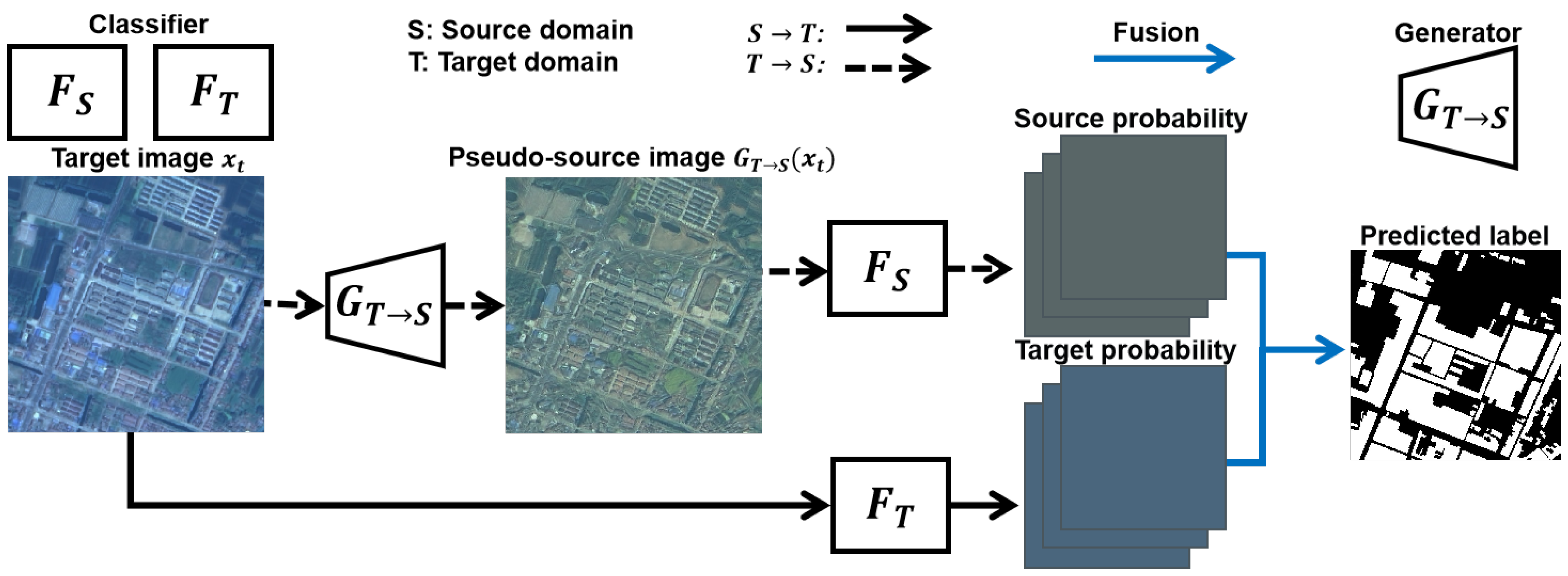
3.4. Linear Combination Method

The target classifier $F_T$ is trained on the pseudo-target domain which have data distributions similar to the target domain and segment the target images. The source segmentation model $F_S$ is optimized on the source domain and segment the pseudo-source images $G_{T\to S}\left(x_t\right)$. These two classifiers make different types of mistakes and assign different confidence ranks to the predicted labels. All in all, the predicted labels of the two classifiers are complementary instead of alternative. When addressing fusion, it is important to stress that we should remove the wrong objects from both predicted labels as much as possible and preserve the correct objects at the same time. For this purpose, we design a simple method which linearly combines their probability output as follows:

$$output=\lambda F_S\left(G_{T\to S}\left(x_t\right)\right)+(1-\lambda )F_T\left(x_t\right)$$

(17)

where $\lambda$ is a hyperparameter in the range $(0,1)$.

Then, we convert the probability output to the predicted labels. A schematic illustration of the linear combination method is shown in Figure 3.

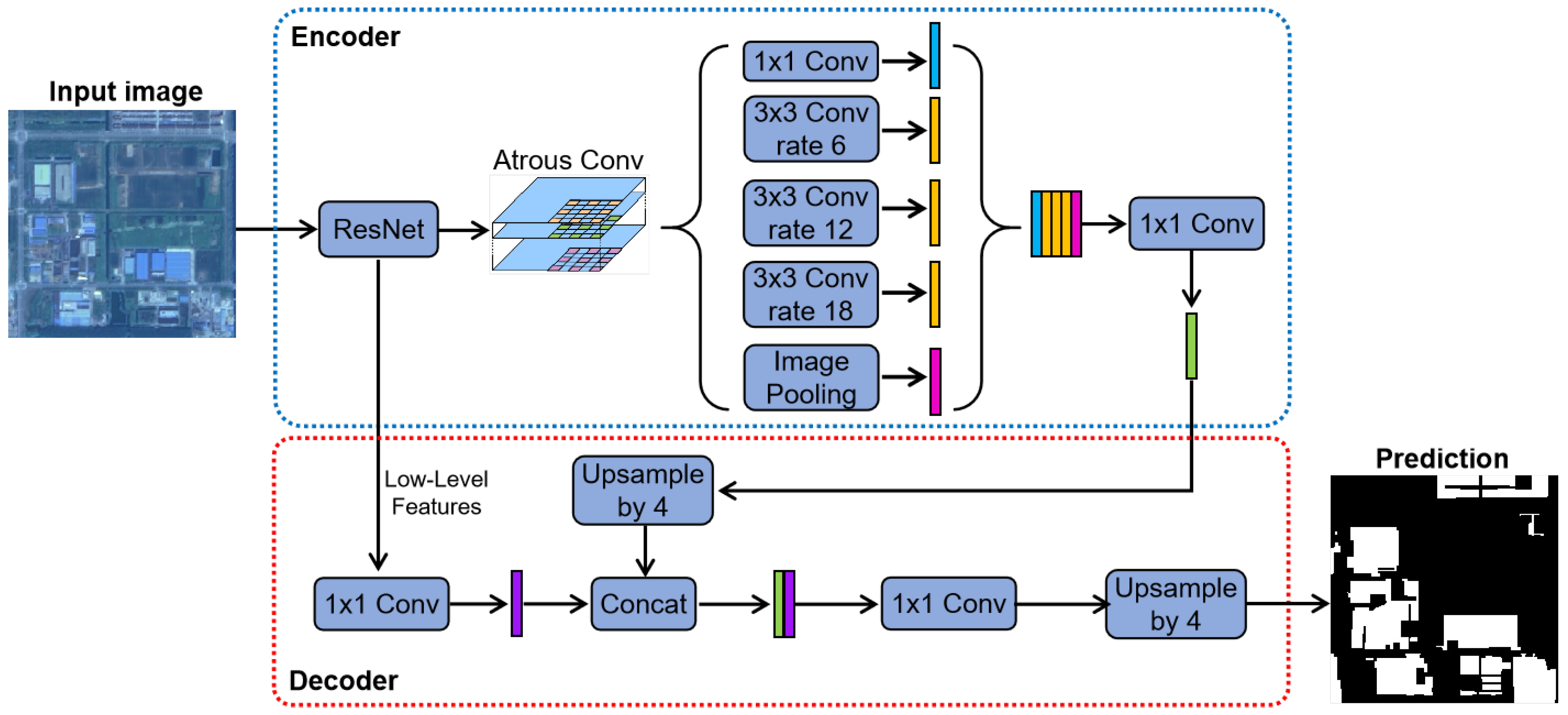
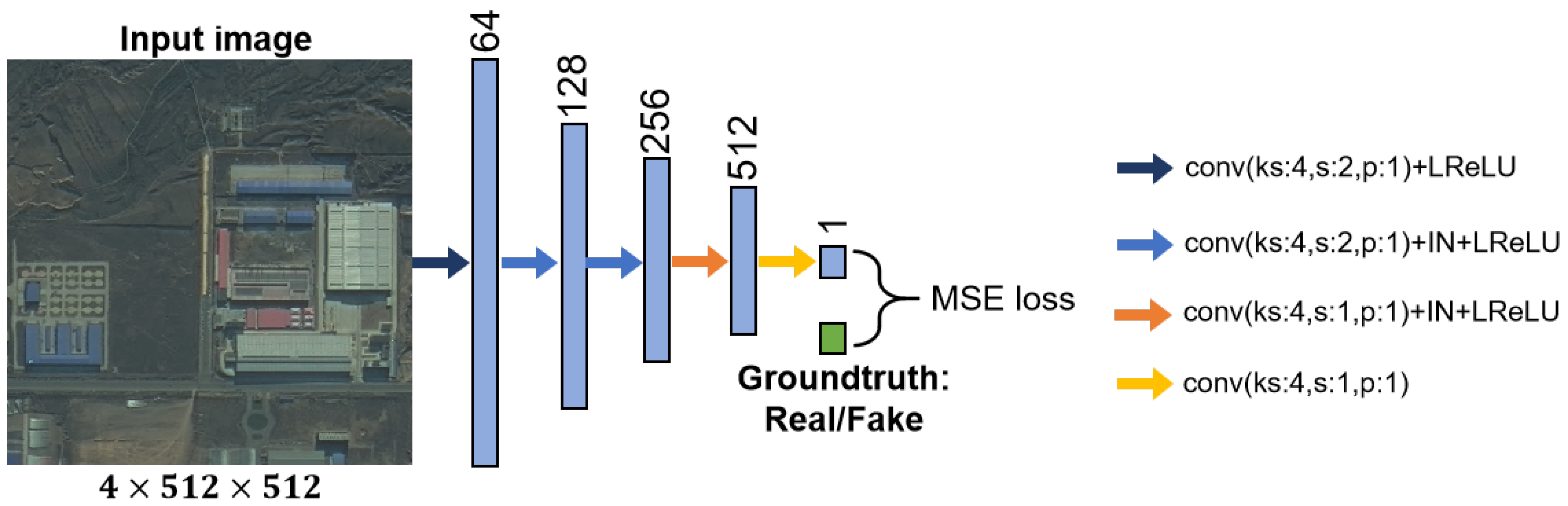
3.5. Network Architecture

Our proposed BiFDANet consists of two generators, two discriminators and two classifiers.

We choose DeeplabV3+ [7] as the segmentation model and use ResNet34 [59] as the DeeplabV3+ backbone. The encoder applies atrous convolution at multiple scales to acquire multi-scale features. The decoder module which is simple yet effective provides the predicted results. We use dropout in the decoder module to avoid overfitting. Figure 4 shows the architecture of the classifier.

As shown in Figure 5, we use nine residual blocks for the generators which are used in [17]. Four convolutional layers are used to downsample the features, while four deconvolutional layers are applied to upsample the features. We use instance normalization rather than batch normalization and we apply ReLU to activate all layers.

Similar to the discriminator in [17], we use five convolution layers for discriminators as shown in Figure 6. The discriminators encode the input images into a feature vector. Then, we compute the mean squared error loss instead of using Sigmoid to convert the feature vector into a binary output (real or fake). We use instance normalization rather than batch normalization. Unlike the generator, leaky ReLU is applied to activate the layers of the discriminator.

4. Results

In this section, we introduce the two datasets, illustrate the experimental settings, and analyse the obtained results both quantitatively and qualitatively.

4.1. Data Set

To conduct our experiments, we employ the Gaofen Satellite dataset and the ISPRS (WGII/4) 2D semantic segmentation benchmark dataset [60]. In the rest of this paper, we abbreviate the Gaofen Satellite data and the ISPRS (WGII/4) 2D semantic segmentation benchmark dataset to the Gaofen dataset and the ISPRS data set to simplify the description.

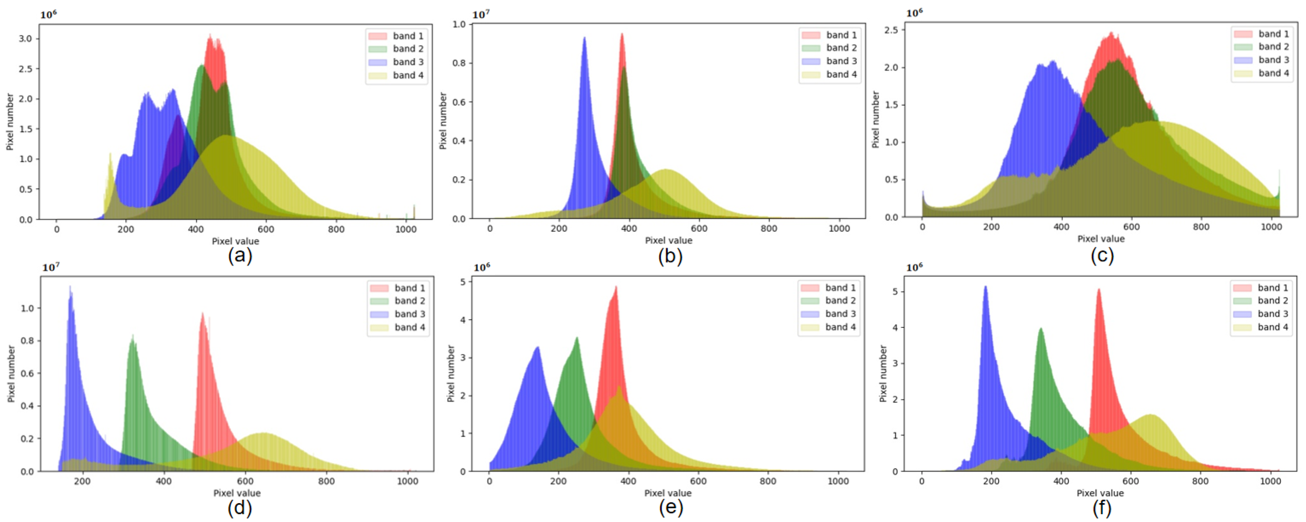
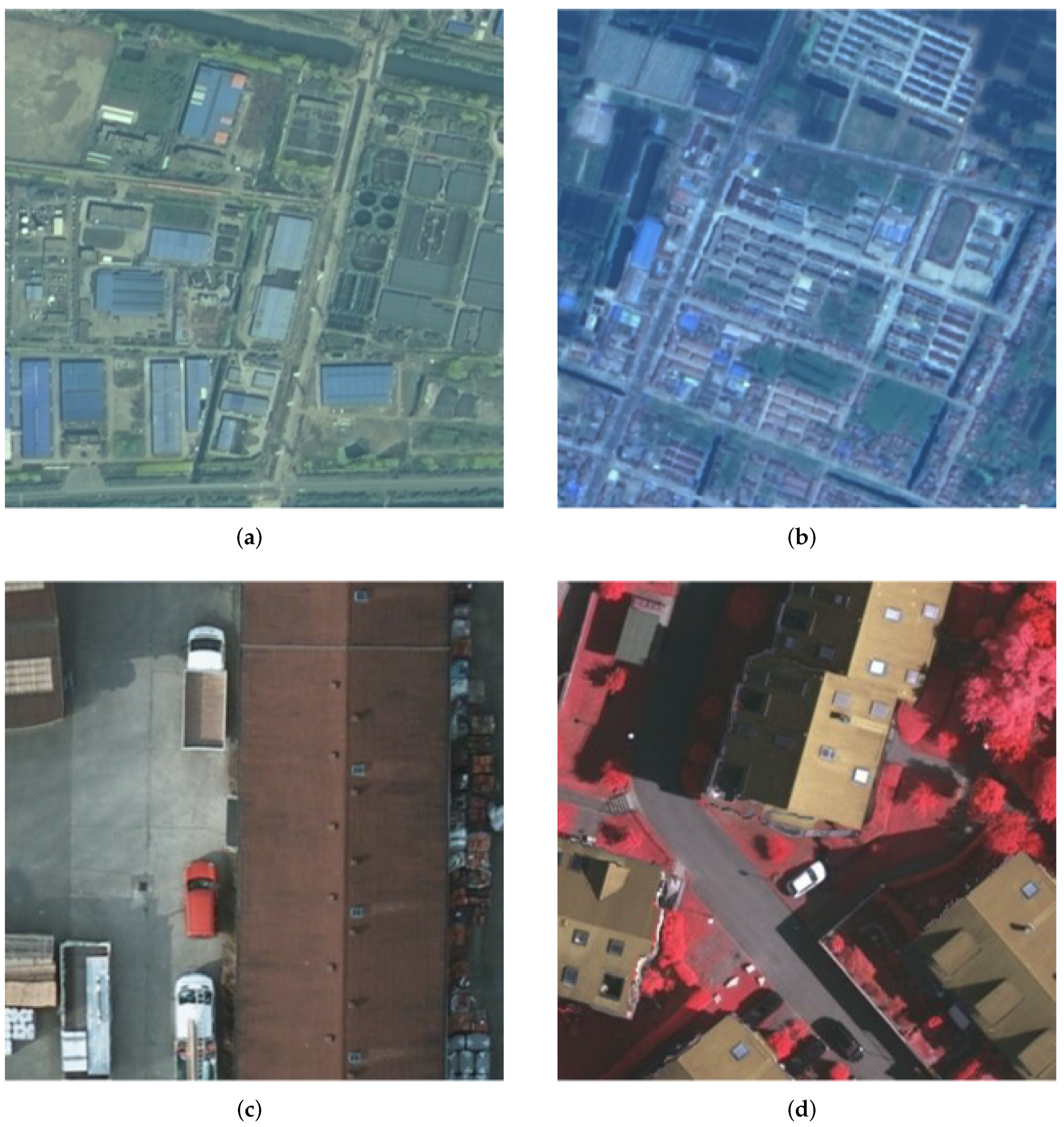
4.1.1. Gaofen Data Set

The Gaofen dataset consists of the Gaofen-1 (GF-1) satellite images and the Gaofen-1B (GF-1B) satellite images, which are civilian optical satellites of China and equipped with two sets of multi-spectral and panchromatic cameras. We reduce spatial resolution of the images to 2 m and convert the images to 10 bit. The images from both satellites contain 4 channels (i.e., red, green, blue and near-infrared). The labels of buildings are provided. We assume that only the labels of the source domain can be accessed. We cut the images and their labels into 512 × 512 patches.

Table 1. Statistics For Data Set.

Image	# of Patches	Patch Size	Class Percentages
GF-1	2039	512 × 512	12.6%
GF-1B	4221	512 × 512	5.4%
Potsdam	4598	512 × 512	28.1%
Vaihingen	459	512 × 512	26.8%

reports the number of patches and the class percentages belonging to each satellite. Figure 7a,b show samples from the GF-1 satellite and the GF-1B satellite.

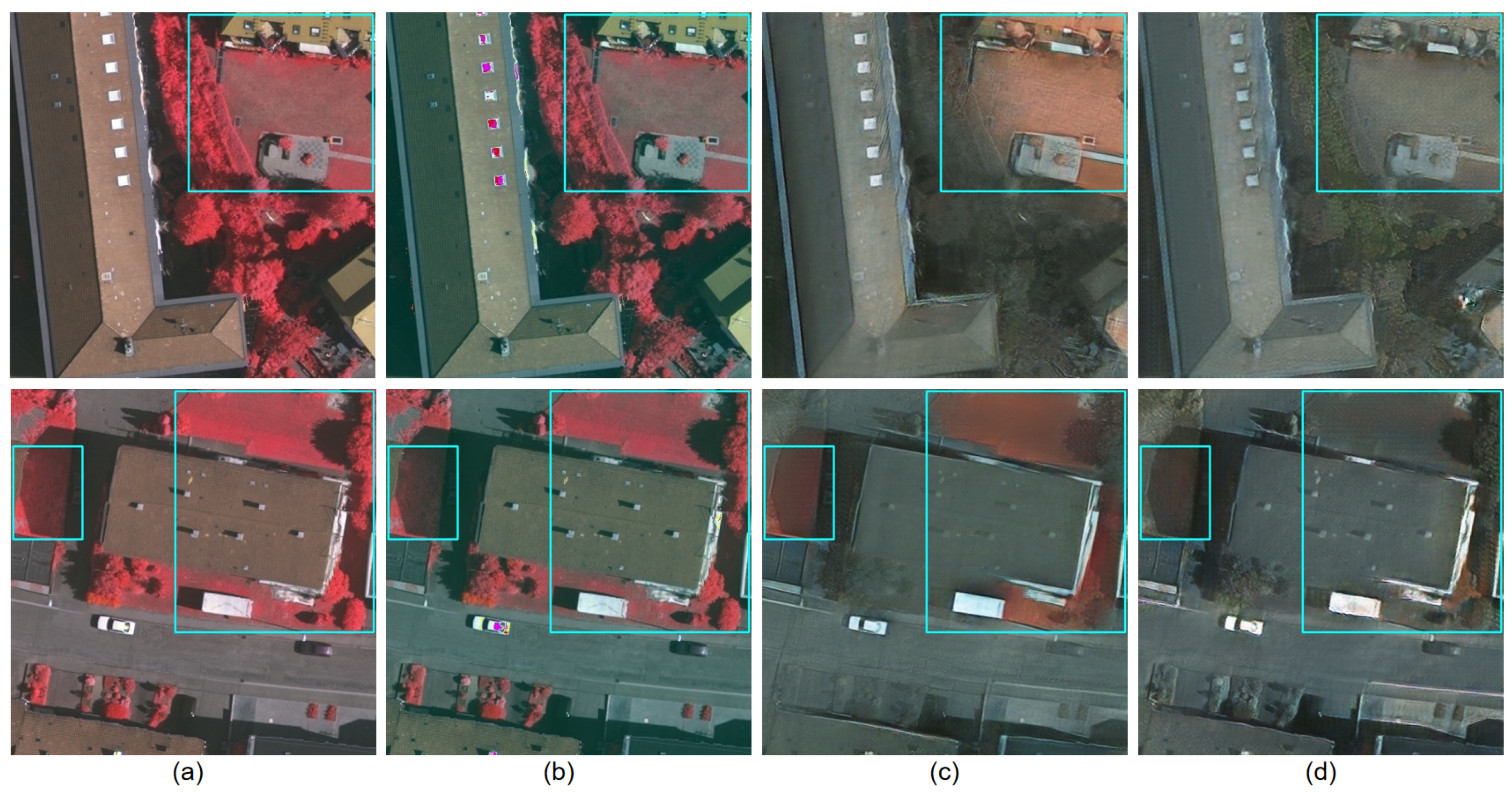
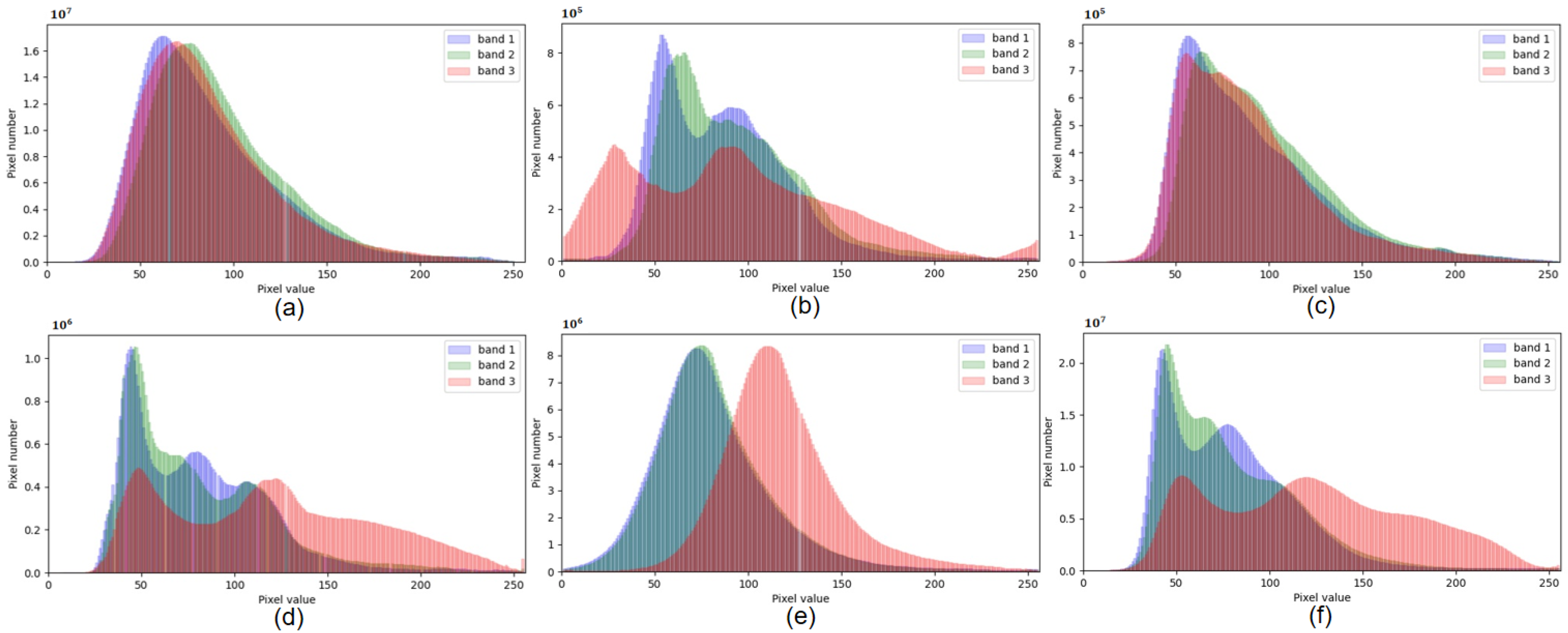
4.1.2. ISPRS Data Set

This ISPRS dataset includes aerial images acquired from [61,62], which have been publicly available to the community. The Vaihingen dataset consists of images with a spatial resolution of 0.09 m and the spatial resolution of Potsdam dataset is 0.05 m. The Potsdam images contain red, green and blue channels while the Vaihingen images have 3 different channels (i.e., red, green and infrared). All images in both datasets are converted to 8 bit. Some images are manually labeled with land cover maps and the labels of impervious surfaces, buildings, trees, low vegetations and cars are provided. We cut the images and their labels into 512 × 512 patches. Table 1 reports the number of patches and the class percentages for the ISPRS dataset. Figure 7c,d show samples from each city.

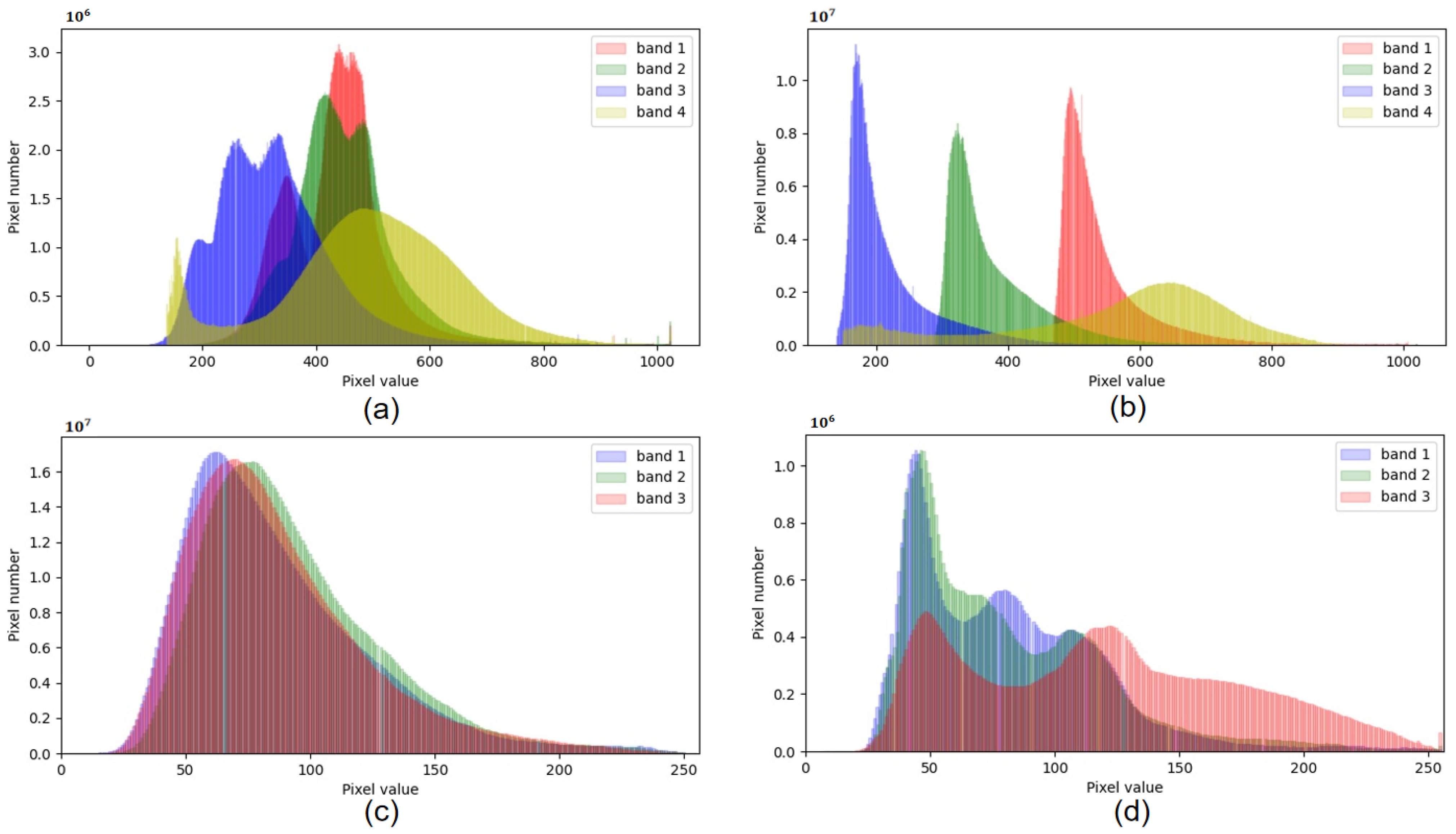
4.1.3. Domain Gap Analysis

The domain shift between different domains is caused by many factors such as illumination conditions, camera angle, imaging sensors and so on.

In terms of the Gaofen data set, the same objects (e.g., buildings) have similar structures, but the colors of the GF-1 satellite images are different from the colors of the GF-1B satellite images as shown in Figure 7a,b. What’s more, we depict the histograms to represent the data distributions of the two datasets. There are some differences between the histograms of the GF-1 satellite images and the GF-1B satellite images as shown in Figure 8a,b.

In terms of the ISPRS dataset, the Potsdam images and the Vaihingen images have many differences, such as imaging sensors, spatial resolutions and structural representations of the classes. The Potsdam images and the Vaihingen images contain different kinds of channels due to the different imaging sensors, which results in the same objects in the two datasets being of different colors. For example, the vegetations and trees are green in the Potsdam dataset while the vegetations and trees are red color because of the infrared band. Besides, the Potsdam images and the Vaihingen images are captured using various spatial resolutions, which leads to the same objects being of different sizes. What’s more, the structural representations of the same objects in the Potsdam dataset and Vaihingen dataset might be different. For example, there may be some differences between the buildings in different cities. At the same time, we depict the histograms to represent the data distributions of the Potsdam dataset and Vaihingen dataset as well. As shown in Figure 8c,d, the histograms of the Potsdam images are quite different from the histograms of the Vaihingen images.

4.2. Experimental Settings

We train BiFDANet in two stages. First, the training process minimizes the overall objective ${\mathcal{L}}_{BiFDANet}(G_{S\to T},G_{T\to S},D_S,D_T,F_S,F_T)$ without the bidirectional semantic consistency loss by setting ${\lambda }_4$ parameters in Equation (15) to 0. This is because, without a trained target segmentation model, the bidirectional semantic consistency loss would not be helpful in training process. The ${\lambda }_1$, ${\lambda }_2$, ${\lambda }_3$, ${\lambda }_5$ and ${\lambda }_6$ parameters in Equation (15) are set to 1, 10, 5, 10 and 10, respectively. We have found these values through repeated experiments. We train the framework for 100 epochs in this step. Second, after we obtain the well-trained target classifier, we add the bidirectional semantic consistency loss by setting ${\lambda }_4$ to 10 and the ${\lambda }_1$, ${\lambda }_2$, ${\lambda }_3$, ${\lambda }_5$ and ${\lambda }_6$ parameters in Equation (15) are the same as in the first step. We then optimize the network for 200 epochs. For all the methods, the networks are implemented in the PyTorch framework. We trained the models with Adam optimizer [63], using a batch size of 12. The learning rates for the generators, the discriminators and the classifiers are all set to ${10}^{-4}$. At test time, the parameters to combine the segmentation models are $\lambda \in [0,0.05,0.1,0.15,0.2,...,0.95,1]$ chosen on the validation set of 20% patches from the target domain.

4.3. Methods Used for Comparison

(1) DeeplabV3+ [7]: We do not apply any domain adaptation methods and directly segment the unlabeled target images with a DeeplabV3+ trained on the labeled source domain.

(2) Color Matching: For each channel of the images, we adjust the average brightness values of the source images to that of the target images. Then, we train the target segmentation model on the transformed domain.

(3) CycleGAN [17]: This method uses two generators G and F to perform image translation. The generator G learns to transfer the source images to the target domain while F learns to transfer the target images to the source domain. This method forces the transferring from source to target and back and transferring from target to source and back reproduce the original contents. Then the generated target-like images are used to train the target classifier.

(4) For BiFDANet, besides the full approach, we also give the results obtained by the segmentation models $F_S$ and $F_T$ before the linear combination method. At the same time, to show the effectiveness of the linear combination method, we also show the results obtained by simply taking the intersection or union of the two results.

For the above approaches, we use the same training parameters and architecture to make a fair comparison.

4.4. Evaluation Metrics

To evaluate all the methods quantitatively and comprehensively, we use scalar metrics included Precision, Recall, F1-score (F1) and IoU [64] defined as follows:

$$Precision=\frac{T{P}_b}{T{P}_b+F{P}_b}$$

(18)

$$Recall=\frac{T{P}_b}{T{P}_b+F{N}_b}$$

(19)

$$F1=\frac{2\times Precision\times Recall}{Precision+Recall}$$

(20)

$$IoU=\frac{T{P}_b}{T{P}_b+F{N}_b+F{P}_b}$$

(21)

where b denotes the category. FP (false positive) is the number of pixels which are classified as category b but do not belong to category b. FN (false negative) corresponds to the number of pixels which are category b but classified as other categories. TP (true positive) is the number of pixels which are correctly classified as category b and TN (true negative) corresponds to the number of pixels which are classified as other categories and belong to other categories. The aforementioned evaluation metrics are computed for each category (except the background). Especially, because we only segment buildings in our experiments, all the evaluation results we reported in tables are corresponding to the building (category).

4.5. Quantitative Results

To report fair and reliable results, we repeat training our framework and the comparison methods with the same parameters and architecture five times and depict the average precision, recall, F1-score and IoU values in

Table 2. Comparison results on Gaofen dataset. The best values are in bold.

Method	Source: GF-1, Target: GF-1B				Source: GF-1B, Target: GF-1
	Recall (%)	Precision (%)	F1 (%)	IoU (%)	Recall (%)	Precision (%)	F1 (%)	IoU (%)
DeeplabV3+	74.78	16.60	27.16	15.72	2.14	70.07	4.17	2.13
Color matching	53.82	55.65	54.72	37.66	49.00	83.64	61.80	44.71
CycleGAN	54.72	67.31	60.37	43.24	60.74	75.12	67.17	50.57
BiFDANet $F_S$	58.56	69.34	63.50	46.52	71.65	72.21	71.93	56.17
BiFDANet $F_T$	61.82	67.00	64.31	47.39	71.81	73.69	72.74	57.16
$F_S\cap F_T$	57.12	70.99	63.31	46.31	67.90	75.77	71.62	55.79
$F_S\cup F_T$	60.92	68.11	64.32	47.40	71.94	73.88	72.90	57.36
BiFDANet	63.31	65.70	64.48	47.58	75.57	70.58	72.99	57.47

and

Table 3. Comparison results on ISPRS dataset. The best values are in bold.

Method	Source: Vaihingen, Target: Potsdam				Source: Potsdam, Target: Vaihingen
	Recall (%)	Precision (%)	F1 (%)	IoU (%)	Recall (%)	Precision (%)	F1 (%)	IoU (%)
DeeplabV3+	30.10	17.81	22.37	12.59	29.64	33.16	31.30	18.55
Color matching	39.27	54.28	45.57	29.51	42.61	36.13	39.11	24.30
CycleGAN	61.13	55.86	58.38	41.22	49.75	66.44	56.90	39.76
BiFDANet $F_S$	68.82	61.62	65.02	48.17	59.00	75.39	66.20	49.47
BiFDANet $F_T$	56.90	62.39	59.52	42.37	60.44	76.70	67.60	51.06
$F_S\cap F_T$	52.35	69.27	59.63	42.48	53.60	79.67	64.09	47.15
$F_S\cup F_T$	73.37	57.63	64.55	47.66	59.95	77.12	67.46	50.90
BiFDANet	66.37	64.03	65.18	48.35	65.83	73.33	69.38	53.12

. Table 2 and Table 3 show the comparison results on the Gaofen dataset and the ISPRS dataset, respectively. The DeeplabV3+ row includes results are corresponding to the no-adaptation case. For BiFDANet, we report the results obtained by the source classifier $F_S$ and the target classifier $F_T$ separately before the linear combination method and obtained by simply taking the intersection or union of the predicted results of the two classifiers $F_S$ and $F_T$.

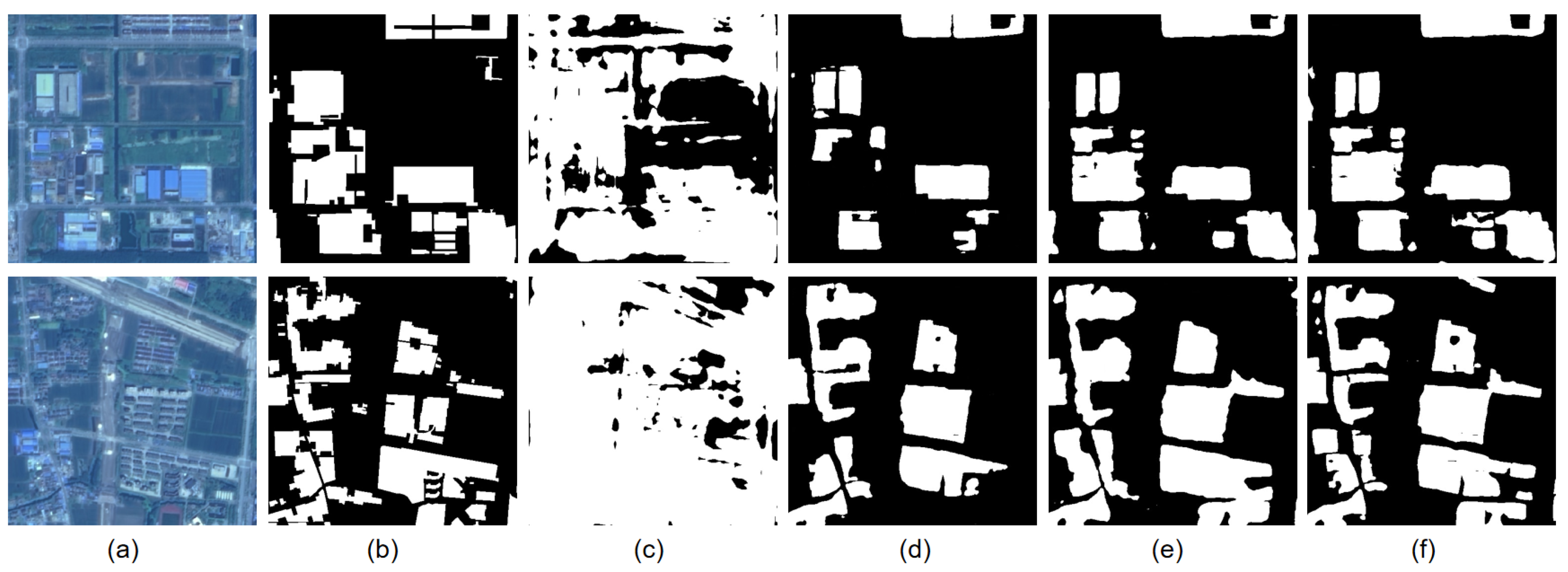
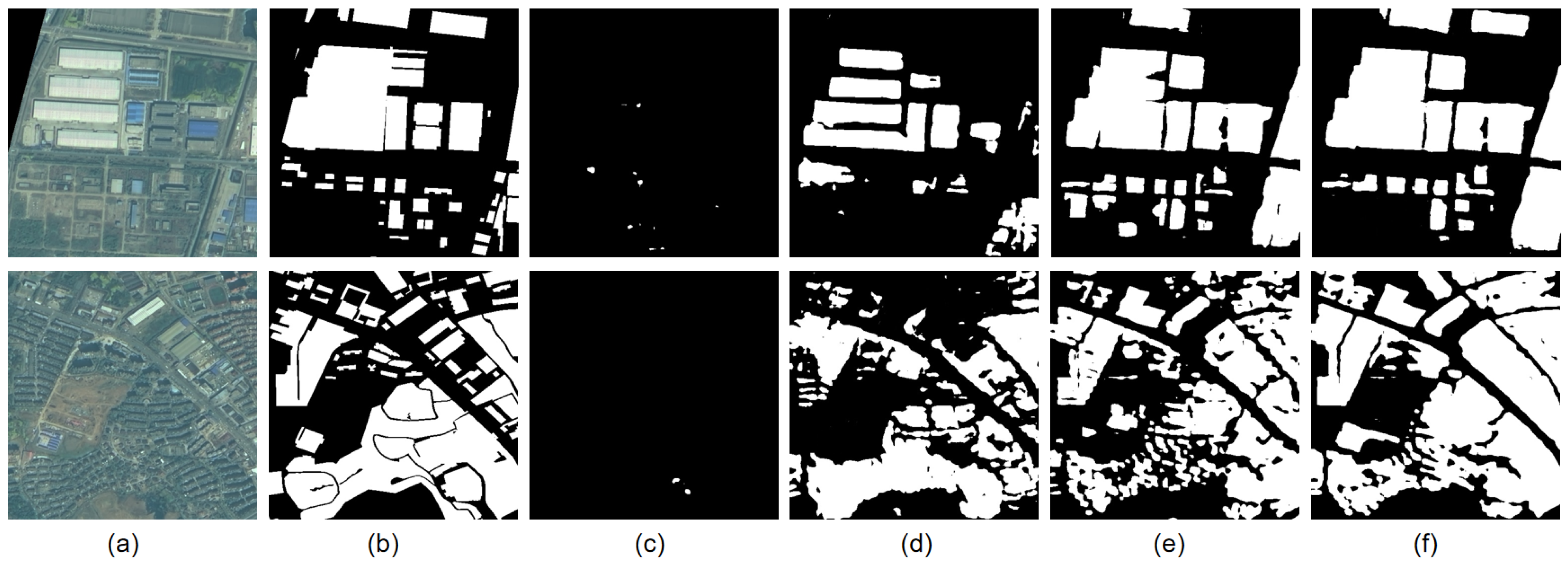
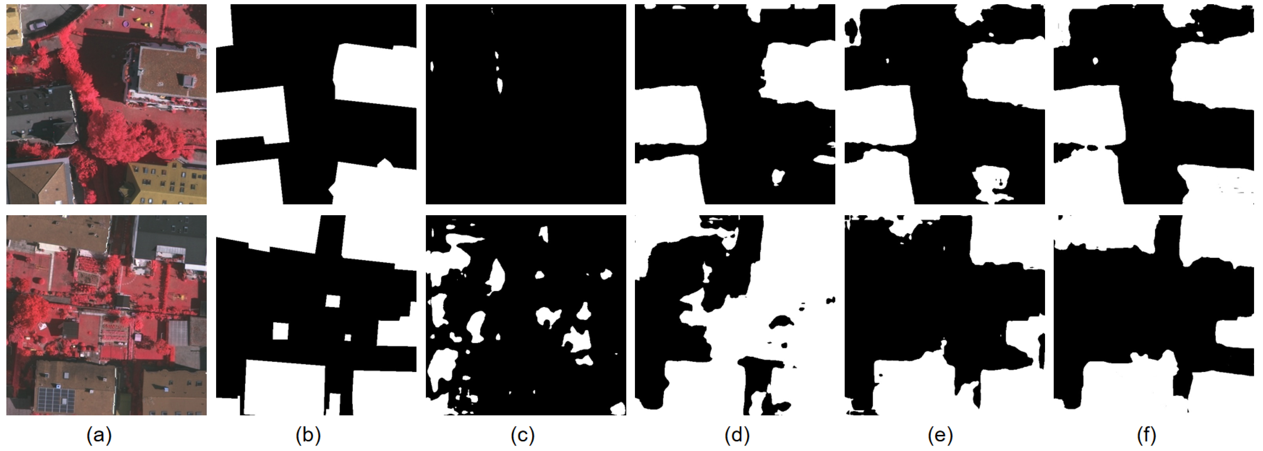
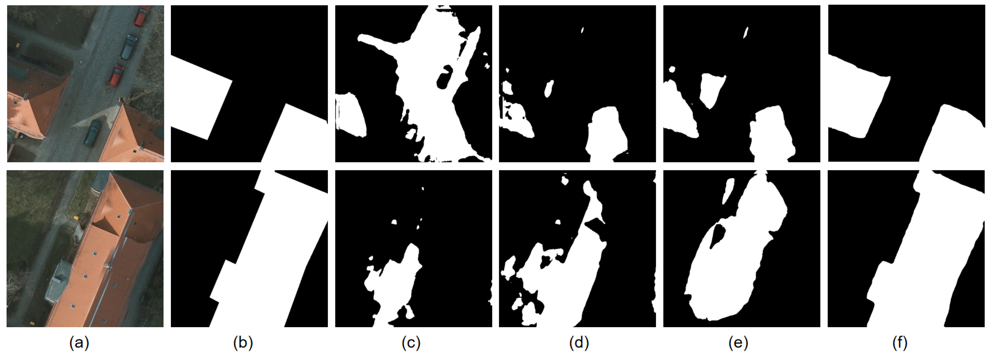
4.6. Visualization Results

Figure 9, Figure 10, Figure 11 and Figure 12 depict the predicted results for DeeplabV3+, CycleGAN, color matching and BiFDANet. Our proposed BiFDANet which considers distribution alignment and bidirectional semantic consistency obtains the best predicted results, and the contours of the predicted buildings are more accurate than those acquired by color matching and CycleGAN.

5. Discussion

In this section, we compare our results with the compared methods in detail, and discuss the effect of our proposed bidirectional semantic consistency (BSC) loss and the roles of each component in our BiFDANet.

5.1. Comparisons with Other Methods

As shown in Table 2 and Table 3, the DeeplabV3+ method which directly apply the source segmentation model to classify the target images performs worst in all settings. Color matching obtains a better performance than the DeeplabV3+ method, which indicates the effectiveness of domain adaptation for semantic segmentation of remote sensing images. CycleGAN perform better than both DeeplabV3+ and Color matching. Among all the compared methods, BiFDANet achieves the highest F1-score and IoU score in all settings. And the separate segmentation models $F_S$ and $F_T$ also significantly outperform the other adaptation methods. When combing the two segmentation models with the linear combination method, the performance of BiFDANet is further enhanced. Moreover, in the Vaihingen → Potsdam experiment, BiFDANet $F_S$ performs much better than BiFDANet $F_T$. Because transferring from Vaihingen to Potsdam is more difficult than transferring from Potsdam to Vaihingen. There are far more Potsdam images than Vaihingen images, in some ways, the widely variable target domain (Potsdam) contains more variety of shapes and textures, and therefore it is more difficult to adapt the classifier from Vaihingen to Potsdam. Thanks to its bidirectionality which is disregarded in previous methods, BiFDANet achieves a performance gain of +7 percentage points while the gain in performance of BiFDANet $F_T$ is only +1 percentage points. In this experiment, our proposed method makes full use of the information from the inverse target-to-source translation to produce much better results.

5.1.1. BiFDANet versus DeeplabV3+

There is no doubt that BiFDANet performs much better than DeeplabV3+ for all four cases. Because of the domain gap, there are some significant differences between the source domain and target domain. Without domain adaptation, the segmentation model cannot deal with the domain gap.

5.1.2. BiFDANet versus CycleGAN

In order to reduce the domain gap, CycleGAN and BiFDANet perform image-to-image translation to align data distribution of different domains. Figure 13, Figure 14, Figure 15 and Figure 16 show some original images and the corresponding transformed images generated by color matching, CycleGAN and BiFDANet. As shown in Figure 13 and Figure 14, it is obvious that the semantic contents of the images are changed by CycleGAN because there are no constraints for CycleGAN to enforce the semantic consistency during the image generation process. For instance, during the translation, CycleGAN replaces the buildings with bare land as shown in Figure 13 and Figure 14 yellow rectangles. Besides, when generating transformed images, CycleGAN produces some buildings which do not exist before, as indicated in Figure 13 and Figure 14 green rectangles. By contrast, the pseudo images transformed by BiFDANet and their corresponding original images have the same semantic contents and the data distributions of the pseudo images are similar to the data distributions of the target images. Similarly, as shown in Figure 15, we observe that there are some objects which look like red trees on the rooftops of the buildings as highlighted by green rectangles. At the same time, the pseudo images transformed by CycleGAN generates a few artificial objects in the outlined areas in Figure 15. What’s more, in Figure 16, the pseudo images transformed by CycleGAN transfer the gray ground to the orange buildings, as highlighted by cyan rectangles. On the contrary, we do not observe aforementioned artificial objects and semantic inconsistency in the transformed images generated by BiFDANet in the vast majority of cases. Because the bidirectional semantic consistency loss enforces the classifiers to maintain semantic consistency during the image-to-image translation process. For CycleGAN, because the transformed images do not match the labels of the original images, the segmentation model $F_T$ learns wrong information in training progress. Such wrong information may affect the performances of classifiers significantly. As a result, the domain adaptation methods with CycleGAN performs worse than our proposed method at test time, as confirmed by Figure 13, Figure 14, Figure 15 and Figure 16.

5.1.3. BiFDANet versus Color Matching

Figure 13 and Figure 14 illustrate that color matching can efficiently reduce the color difference between different domains. At the first sight, color matching works well. It preserves the semantic contents of the original source images in the transformed images, and the color of the target images is transferred to the transformed images. Besides, the transformed images generated by color matching look similar to the images generated by BiFDANet in Figure 14. However, in Table 2 and Table 3, we can see that there are relatively big gaps between the performances of BiFDANet and color matching. The quantitative results for color matching are worse than the results for CycleGAN which can not keep semantic contents well. To better understand why there is such a difference in performance, we further analyse the differences between BiFDANet and color matching. The main problem of color matching is that it only tries to match the color of the images instead of considering the differences in features and data distributions. On the contrary, BiFDANet learns high-level features of the target images by using the discriminators to distinguish the features and data distributions of the pseudo-target transformed images from that of the original target images. In other word, the generators of BiFDANet generate pseudo-target transformed images whose high-level features and data distributions are similar to that of the target images. For this reason, our proposed BiFDANet outperforms color matching substantially.

Furthermore, to prove our point, we show color histograms of the GF-1 images, the pseudo GF-1 images generated by color matching and BiFDANet, and the GF-1B images, the pseudo GF-1B images generated by color matching and BiFDANet in Figure 17. And we depict color histograms of the Potsdam images, the pseudo Potsdam images generated by color matching and BiFDANet, and the Vaihingen images, the pseudo Vaihingen images generated by color matching and BiFDANet in Figure 18. Since the source domain and the target domain are drawn from different data distributions, the histograms of the pseudo-target images and the target images can’t be exactly the same. However, we want them to be as similar as possible. Although color matching tries to match the color of the source images with the color of the target images, it doesn’t learn the data distributions so that the histograms of the pseudo-target images are quite different from that of the target images.

As shown in Figure 17 and Figure 18, color matching does not match the data distributions of the pseudo-target images with the data distributions of the target images. For Gaofen dataset, there are still some differences between the histograms of the pseudo-target images generated by color matching and the real target images as shown in Figure 17. In contrast, the histograms of the pseudo-target images transformed by BiFDANet are similar to that of the real target images as shown in Figure 17. Thus the performances of BiFDANet are better than color matching. For ISPRS dataset, the histograms of the pseudo-target images generated by color matching are much different from the histograms of the target images as shown in Figure 18. In comparison, BiFDANet effectively matches the histograms of pseudo-target images with the histograms of the real target images, as shown in Figure 18. Therefore, the performance gap between BiFDANet and color matching becomes larger as confirmed by Figure 13, Figure 14, Figure 15 and Figure 16.

5.1.4. Linear Combination Method versus Intersection and Union

In the GF-1 → GF-1B, Vaihingen → Potsdam and Potsdam → Vaihingen experiments, simply taking the intersection or union of the results of the two classifiers $F_S$ and $F_T$ obtains the highest precision values or recall values, these results prove that the two opposite directions are complementary instead of alternative. However, the F1-score values and IoU values can’t achieve the highest by the intersection and union operation. In the Vaihingen → Potsdam and Potsdam → Vaihingen experiments, simply taking the intersection or union of the outputs of the two classifiers $F_S$ and $F_T$ results in performance degradation. It shows that the intersection operation and union operation of the two predicted results aren’t always stable, because these methods may leave out some correct objects or introduce some wrong objects during the combination process. In comparison, the linear combination method leads to further improvements for all four experiments because the combination of probability output is more reliable.

5.2. Bidirectional Semantic Consistency Loss

We replace the bidirectional semantic consistency (BSC) loss in BiFDANet with semantic consistency (SC) loss [14] and dynamic semantic consistency (DSC) loss [45], and report the evaluation results in

Table 4. Evaluation results of different semantic consistency loss on Gaofen dataset. The best values are in bold.

Method		Source: GF-1, Target: GF-1B				Source: GF-1B, Target: GF-1
		Recall (%)	Precision (%)	F1 (%)	IoU (%)	Recall (%)	Precision (%)	F1 (%)	IoU (%)
BiFDANet w/o	$F_S$	55.68	62.07	58.70	41.55	65.36	67.21	66.27	49.68
	$F_T$	52.97	70.69	60.56	43.43	65.80	70.63	68.13	51.53
	BiFDANet	54.83	68.83	61.04	43.92	67.10	69.86	68.45	51.87
BiFDANet w/SC	$F_S$	50.84	73.68	60.16	43.02	69.43	68.36	68.89	52.33
	$F_T$	57.76	68.39	62.63	45.59	65.28	74.48	69.58	53.35
	BiFDANet	56.10	71.21	62.76	45.73	66.67	73.20	69.78	53.59
BiFDANet w/DSC	$F_S$	53.66	69.36	60.51	43.38	68.14	70.36	69.23	52.84
	$F_T$	59.90	66.69	63.11	46.11	70.44	73.24	71.81	56.02
	BiFDANet	58.47	70.23	63.81	46.86	72.34	71.93	72.13	56.41
BiFDANet w/BSC	$F_S$	58.56	69.34	63.50	46.52	71.65	72.21	71.93	56.17
	$F_T$	61.82	67.00	64.31	47.39	71.81	73.69	72.74	57.16
	BiFDANet	63.31	65.70	64.48	47.58	75.57	70.58	72.99	57.47

and

Table 5. Evaluation results of different semantic consistency loss on ISPRS dataset. The best values are in bold.

Method		Source: Vaihingen, Target: Potsdam				Source: Potsdam, Target: Vaihingen
		Recall (%)	Precision (%)	F1 (%)	IoU (%)	Recall (%)	Precision (%)	F1 (%)	IoU (%)
BiFDANet w/o	$F_S$	49.37	72.12	58.62	41.46	45.81	71.71	55.91	38.80
	$F_T$	44.60	73.89	55.63	38.53	47.30	72.32	57.19	40.05
	BiFDANet	51.39	68.75	58.81	41.66	48.41	72.67	58.11	40.96
BiFDANet w/SC	$F_S$	52.72	72.96	61.21	44.10	53.69	69.82	60.70	43.58
	$F_T$	49.71	72.20	58.88	41.73	56.05	72.89	63.37	46.38
	BiFDANet	53.83	71.97	61.59	44.50	60.35	67.40	63.68	46.71
BiFDANet w/DSC	$F_S$	58.93	67.35	62.86	45.84	58.01	68.30	62.74	45.70
	$F_T$	50.66	70.76	59.05	41.89	60.53	74.44	66.77	50.11
	BiFDANet	53.03	77.84	63.08	46.07	62.75	73.13	67.54	50.99
BiFDANet w/BSC	$F_S$	68.82	61.62	65.02	48.17	59.00	75.39	66.20	49.47
	$F_T$	56.90	62.39	59.52	42.37	60.44	76.70	67.60	51.06
	BiFDANet	66.37	64.03	65.18	48.35	65.83	73.33	69.38	53.12

.

As shown in Table 4 and Table 5, we can see that for all adaptations in both directions on Gaofen data set and ISPRS data set, our proposed bidirectional semantic consistency loss achieves better results. It is worth noting that our framework with SC loss [14] and DSC loss [45] also performs well in the source-to-target direction, but the performance of $BiFDANet$ $F_S$ degrades. This illustrates the necessity of the proposed bidirectional semantic consistency loss when optimizing the classifier $F_S$ in the target-to-source direction. What’s more, our framework with the proposed bidirectional semantic consistency (BSC) loss outperforms our framework with the dynamic semantic consistency (DSC) loss in the source-to-target direction even if the semantic constraints are the same in this direction. It shows that keeping semantic consistency in the target-to-source direction is helpful to maintain the semantic consistency in the source-to-target direction. At the same time, the source classifier $F_S$ in our framework with semantic consistency loss [14] and dynamic semantic consistency loss [45] perform better than the source classifier $F_S$ in our framework without semantic consistency loss even though there are no semantic constraints for these methods in the target-to-source direction. It means that the semantic consistency constraints in the source-to-target direction are also beneficial to preserve the semantic contents in the target-to-source direction. In conclusion, these two transferring directions promote each other to keep the semantic consistency.

5.3. Loss Functions

We study the roles of each part in BiFDANet in the Vaihingen → Potsdam experiment. We start from the base source-to-target GAN model with the adversarial loss ${\mathcal{L}}_{adv}$ and the classification loss ${\mathcal{L}}_{F_T}$. Then we test the symmetric target-to-source GAN model with the adversarial loss ${\mathcal{L}}_{adv}$ and the classification loss ${\mathcal{L}}_{F_S}$. We combine the two symmetric models that form a closed loop. In the next steps, we add the cycle consistency loss ${\mathcal{L}}_{cyc}$ and the identity loss ${\mathcal{L}}_{idt}$ in turn. Finally, the framework is completed by introducing the bidirectional semantic consistency loss ${\mathcal{L}}_{sem}$. The results are shown in

Table 6. Evaluation results of each component on ISPRS dataset.

Source: Vaihingen, Target: Potsdam
$\mathit{S}\to \mathit{T}$					$\mathit{T}\to \mathit{S}$					F1 (%)	IoU (%)
${\mathcal{L}}_{{\mathit{F}}_{\mathit{T}}}$	${\mathcal{L}}_{\mathit{a}\mathit{d}\mathit{v}}$	${\mathcal{L}}_{\mathit{c}\mathit{y}\mathit{c}}$	${\mathcal{L}}_{\mathit{i}\mathit{d}\mathit{t}}$	${\mathcal{L}}_{\mathit{s}\mathit{e}\mathit{m}}$	${\mathcal{L}}_{{\mathit{F}}_{\mathit{S}}}$	${\mathcal{L}}_{\mathit{a}\mathit{d}\mathit{v}}$	${\mathcal{L}}_{\mathit{c}\mathit{y}\mathit{c}}$	${\mathcal{L}}_{\mathit{i}\mathit{d}\mathit{t}}$	${\mathcal{L}}_{\mathit{s}\mathit{e}\mathit{m}}$
✓	✓									35.67	18.65
					✓	✓				39.84	23.63
✓	✓				✓	✓				40.17	24.08
✓	✓	✓								55.24	38.16
					✓	✓	✓			56.73	39.64
✓	✓	✓			✓	✓	✓			57.04	40.06
✓	✓	✓	✓							54.36	37.83
					✓	✓	✓	✓		57.74	40.12
✓	✓	✓	✓		✓	✓	✓	✓		58.81	41.66
✓	✓	✓	✓	✓						58.44	41.54
					✓	✓	✓	✓	✓	63.96	47.08
✓	✓	✓	✓	✓	✓	✓	✓	✓	✓	65.18	48.35

. We can observe that all components help our framework to achieve better IoU and F1 scores, and the proposed bidirectional semantic consistency loss could further improve the performance of the models, which demonstrates the effectiveness of our bidirectional semantic consistency loss again.

6. Conclusions

In this article, we present a novel unsupervised bidirectional domain adaptation framework to overcome the limitations of the unidirectional methods for semantic segmentation in remote sensing. First, while the unidirectional domain adaptation methods do not consider the inverse adaptation, we take full advantage of the information from both domains by performing bidirectional image-to-image translation to minimize the domain shift and optimizing the source and target classifiers in two opposite directions. Second, the unidirectional domain adaptation methods may perform badly when transferring from one domain to the other domain is difficult. In order to make the framework more general and robust, we employ a linear combination method at test time, which linearly merge the softmax output of two segmentation models, providing a further gain in performance. Finally, to keep the semantic contents in the target-to-source direction which was neglected by the existing methods, we propose a novel bidirectional semantic consistency loss and supervise the translation in both directions. We validate our framework on two remote sensing datasets, consisting of the satellite images and the aerial images, where we perform a one-to-one domain adaptation in each dataset in two opposite directions. The experimental results confirm the effectiveness of our BiFDANet. Furthermore, the analysis reveals the proposed bidirectional semantic consistency loss performs better than other semantic consistency losses used in the previous approaches. In our future work, we will redesign the combination method to make our framework more robust and further improve the segmentation accuracy. What’s more, in practical terms, the huge number of remote sensing images usually contain several domains, we will extend our approach to multi-source and multi-target domain adaptation.

References

1. Chen, Z.; Li, D.; Fan, W.; Guan, H.; Wang, C.; Li, J. Self-Attention in Reconstruction Bias U-Net for Semantic Segmentation of Building Rooftops in Optical Remote Sensing Images. Remote Sens. 2021, 13, 2524. [Google Scholar] [CrossRef]
2. Kou, R.; Fang, B.; Chen, G.; Wang, L. Progressive Domain Adaptation for Change Detection Using Season-Varying Remote Sensing Images. Remote Sens. 2020, 12, 3815. [Google Scholar] [CrossRef]
3. Ma, C.; Sha, D.; Mu, X. Unsupervised Adversarial Domain Adaptation with Error-Correcting Boundaries and Feature Adaption Metric for Remote-Sensing Scene Classification. Remote Sens. 2021, 13, 1270. [Google Scholar] [CrossRef]
4. Krizhevsky, A.; Sutskever, I.; Hinton, G.E. ImageNet Classification with Deep Convolutional Neural Networks. In Proceedings of the International Conference on Neural Information Processing Systems (NIPS), Lake Tahoe, NV, USA, 3–6 December 2012; pp. 1097–1105. [Google Scholar]
5. Chen, L.C.; Papandreou, G.; Kokkinos, I.; Murphy, K.; Yuille, A.L. DeepLab: Semantic Image Segmentation with Deep Convolutional Nets, Atrous Convolution, and Fully Connected CRFs. IEEE Trans. Pattern Anal. Mach. Intell. 2018, 40, 834–848. [Google Scholar] [CrossRef]
6. Chen, L.C.; Papandreou, G.; Schroff, F.; Adam, H. Rethinking Atrous Convolution for Semantic Image Segmentation. arXiv 2017, arXiv:1706.05587. [Google Scholar]
7. Chen, L.C.; Zhu, Y.; Papandreou, G.; Schroff, F.; Adam, H. Encoder-Decoder with Atrous Separable Convolution for Semantic Image Segmentation. In Proceedings of the European Conference on Computer Vision (ECCV), Munich, Germany, 8–14 September 2018; pp. 801–818. [Google Scholar]
8. Tuia, D.; Persello, C.; Bruzzone, L. Domain Adaptation for the Classification of Remote Sensing Data: An Overview of Recent Advances. IEEE Geosci. Remote Sens. Mag. 2016, 4, 41–57. [Google Scholar] [CrossRef]
9. Buslaev, A.; Iglovikov, V.I.; Khvedchenya, E.; Parinov, A.; Druzhinin, M.; Kalinin, A.A. Albumentations: Fast and Flexible Image Augmentations. Informatic 2020, 11, 125. [Google Scholar] [CrossRef] [Green Version]
10. Stark, J.A. Adaptive Image Contrast Enhancement Using Generalizations of Histogram Equalization. IEEE Trans. Image Process. 2000, 9, 889–896. [Google Scholar] [CrossRef] [PubMed] [Green Version]
11. Huang, S.C.; Cheng, F.C.; Chiu, Y.S. Efficient Contrast Enhancement Using Adaptive Gamma Correction With Weighting Distribution. IEEE Trans. Image Process. 2013, 22, 1032–1041. [Google Scholar] [CrossRef] [PubMed]
12. Goodfellow, I.; Pouget-Abadie, J.; Mirza, M.; Xu, B.; Warde-Farley, D.; Ozair, S.; Courville, A.; Bengio, Y. Generative Adversarial Nets. In Proceedings of the International Conference on Neural Information Processing Systems (NIPS), Montreal, QC, Canada, 8–13 December 2014; pp. 2672–2680. [Google Scholar]
13. Sankaranarayanan, S.; Balaji, Y.; Jain, A.; Lim, S.N.; Chellappa, R. Unsupervised Domain Adaptation for Semantic Segmentation with GANs. arXiv 2017, arXiv:1711.06969. [Google Scholar]
14. Hoffman, J.; Tzeng, E.; Park, T.; Zhu, J.Y.; Isola, P.; Saenko, K.; Efros, A.; Darrell, T. CyCADA: Cycle-Consistent Adversarial Domain Adaptation. In Proceedings of the 35th International Conference on Machine Learning (ICML), Stockholm, Sweden, 10–15 July 2018; pp. 1989–1998. [Google Scholar]
15. Tzeng, E.; Hoffman, J.; Saenko, K.; Darrell, T. Adversarial Discriminative Domain Adaptation. In Proceedings of the IEEE Conference on Computer Vision and Pattern Recognition (CVPR), Honolulu, HI, USA, 21–26 July 2017; pp. 7167–7176. [Google Scholar]
16. Benjdira, B.; Bazi, Y.; Koubaa, A.; Ouni, K. Unsupervised Domain Adaptation using Generative Adversarial Networks for Semantic Segmentation of Aerial Images. Remote Sens. 2019, 11, 1369. [Google Scholar] [CrossRef] [Green Version]
17. Zhu, J.Y.; Park, T.; Isola, P.; Efros, A.A. Unpaired Image-to-Image Translation Using Cycle-Consistent Adversarial Networks. In Proceedings of the IEEE International Conference on Computer Vision (ICCV), Venice, Italy, 22–29 October 2017; pp. 2223–2232. [Google Scholar]
18. Rida, I.; Al-Maadeed, N.; Al-Maadeed, S.; Bakshi, S. A comprehensive overview of feature representation for biometric recognition. Multimed. Tools Appl. 2020, 79, 4867–4890. [Google Scholar] [CrossRef]
19. Bruzzone, L.; Persello, C. A Novel Approach to the Selection of Spatially Invariant Features for the Classification of Hyperspectral Images With Improved Generalization Capability. IEEE Trans. Geosci. Remote Sens. 2009, 47, 3180–3191. [Google Scholar] [CrossRef] [Green Version]
20. Persello, C.; Bruzzone, L. Kernel-Based Domain-Invariant Feature Selection in Hyperspectral Images for Transfer Learning. IEEE Trans. Geosci. Remote Sens. 2016, 54, 2615–2626. [Google Scholar] [CrossRef]
21. Rida, I.; Al Maadeed, S.; Bouridane, A. Unsupervised feature selection method for improved human gait recognition. In Proceedings of the 2015 23rd European Signal Processing Conference (EUSIPCO), Nice, France, 31 August–4 September 2015; pp. 1128–1132. [Google Scholar]
22. Hoffman, J.; Wang, D.; Yu, F.; Darrell, T. FCNs in the Wild: Pixel-level Adversarial and Constraint-based Adaptation. arXiv 2016, arXiv:1612.02649. [Google Scholar]
23. Tsai, Y.H.; Hung, W.C.; Schulter, S.; Sohn, K.; Yang, M.H.; Chandraker, M. Learning to Adapt Structured Output Space for Semantic Segmentation. In Proceedings of the IEEE Conference on Computer Vision and Pattern Recognition (CVPR), Salt Lake City, UT, USA, 18–22 June 2018; pp. 7472–7481. [Google Scholar]
24. Zhang, Y.; David, P.; Gong, B. Curriculum Domain Adaptation for Semantic Segmentation of Urban Scenes. In Proceedings of the IEEE International Conference on Computer Vision (ICCV), Venice, Italy, 22–29 October 2017; pp. 2020–2030. [Google Scholar]
25. Zhang, Y.; Qiu, Z.; Yao, T.; Liu, D.; Mei, T. Fully Convolutional Adaptation Networks for Semantic Segmentation. In Proceedings of the IEEE Conference on Computer Vision and Pattern Recognition (CVPR), Salt Lake City, UT, USA, 18–22 June 2018; pp. 6810–6818. [Google Scholar]
26. Bruzzone, L.; Prieto, D.F. Unsupervised Retraining of a Maximum Likelihood Classifier for the Analysis of Multitemporal Remote Sensing Images. IEEE Trans. Geosci. Remote Sens. 2001, 39, 456–460. [Google Scholar] [CrossRef] [Green Version]
27. Bruzzone, L.; Cossu, R. A Multiple-Cascade-Classifier System for a Robust and Partially Unsupervised Updating of Land-Cover Maps. IEEE Trans. Geosci. Remote Sens. 2002, 40, 1984–1996. [Google Scholar] [CrossRef]
28. Chen, Y.; Li, W.; Van Gool, L. ROAD: Reality Oriented Adaptation for Semantic Segmentation of Urban Scenes. In Proceedings of the IEEE Conference on Computer Vision and Pattern Recognition (CVPR), Salt Lake City, UT, USA, 18–22 June 2018; pp. 7892–7901. [Google Scholar]
29. Tasar, O.; Tarabalka, Y.; Giros, A.; Alliez, P.; Clerc, S. StandardGAN: Multi-source Domain Adaptation for Semantic Segmentation of Very High Resolution Satellite Images by Data Standardization. In Proceedings of the IEEE/CVF Conference on Computer Vision and Pattern Recognition Workshops, Seattle, WA, USA, 13–19 June 2020; pp. 192–193. [Google Scholar]
30. Zhang, L.; Zhang, L.; Tao, D.; Huang, X. Sparse Transfer Manifold Embedding for Hyperspectral Target Detection. IEEE Trans. Geosci. Remote Sens. 2014, 52, 1030–1043. [Google Scholar] [CrossRef]
31. Yang, H.L.; Crawford, M.M. Spectral and Spatial Proximity-Based Manifold Alignment for Multitemporal Hyperspectral Image Classification. IEEE Trans. Geosci. Remote Sens. 2016, 54, 51–64. [Google Scholar] [CrossRef]
32. Huang, H.; Huang, Q.; Krahenbuhl, P. Domain Transfer Through Deep Activation Matching. In Proceedings of the European Conference on Computer Vision (ECCV), Munich, Germany, 8–14 September 2018; pp. 590–605. [Google Scholar]
33. Demir, B.; Minello, L.; Bruzzone, L. Definition of Effective Training Sets for Supervised Classification of Remote Sensing Images by a Novel Cost-Sensitive Active Learning Method. IEEE Trans. Geosci. Remote Sens. 2014, 52, 1272–1284. [Google Scholar] [CrossRef]
34. Ghassemi, S.; Fiandrotti, A.; Francini, G.; Magli, E. Learning and Adapting Robust Features for Satellite Image Segmentation on Heterogeneous Data Sets. IEEE Trans. Geosci. Remote Sens. 2019, 57, 6517–6529. [Google Scholar] [CrossRef]
35. Liu, M.Y.; Breuel, T.; Kautz, J. Unsupervised Image-to-Image Translation Networks. In Proceedings of the International Conference on Neural Information Processing Systems (NIPS), Long Beach, CA, USA, 4–9 December 2017; pp. 700–708. [Google Scholar]
36. Huang, X.; Liu, M.Y.; Belongie, S.; Kautz, J. Multimodal Unsupervised Image-to-Image Translation. In Proceedings of the European Conference on Computer Vision (ECCV), Munich, Germany, 8–14 September 2018; pp. 172–189. [Google Scholar]
37. Lee, H.Y.; Tseng, H.Y.; Huang, J.B.; Singh, M.; Yang, M.H. Diverse Image-to-Image Translation via Disentangled Representations. In Proceedings of the European Conference on Computer Vision (ECCV), Munich, Germany, 8–14 September 2018; pp. 35–51. [Google Scholar]
38. Johnson, J.; Alahi, A.; Fei-Fei, L. Perceptual Losses for Real-Time Style Transfer and Super-Resolution. In Proceedings of the European Conference on Computer Vision (ECCV), Amsterdam, The Netherlands, 11–14 October 2016; pp. 694–711. [Google Scholar]
39. Ulyanov, D.; Lebedev, V.; Vedaldi, A.; Lempitsky, V.S. Texture Networks: Feed-forward Synthesis of Textures and Stylized Images. In Proceedings of the International Conference on Machine Learning (ICML), New York, NY, USA, 19–24 June 2016; p. 4. [Google Scholar]
40. Gatys, L.A.; Ecker, A.S.; Bethge, M. Image Style Transfer Using Convolutional Neural Networks. In Proceedings of the IEEE Conference on Computer Vision and Pattern Recognition (CVPR), Las Vegas, NV, USA, 27–30 June 2016; pp. 2414–2423. [Google Scholar]
41. Shrivastava, A.; Pfister, T.; Tuzel, O.; Susskind, J.; Wang, W.; Webb, R. Learning from Simulated and Unsupervised Images through Adversarial Training. In Proceedings of the IEEE Conference on Computer Vision and Pattern Recognition (CVPR), Honolulu, HI, USA, 21–26 July 2017; pp. 2107–2116. [Google Scholar]
42. Bousmalis, K.; Silberman, N.; Dohan, D.; Erhan, D.; Krishnan, D. Unsupervised Pixel-Level Domain Adaptation with Generative Adversarial Networks. In Proceedings of the IEEE Conference on Computer Vision and Pattern Recognition (CVPR), Honolulu, HI, USA, 21–26 July 2017; pp. 3722–3731. [Google Scholar]
43. Murez, Z.; Kolouri, S.; Kriegman, D.; Ramamoorthi, R.; Kim, K. Image to Image Translation for Domain Adaptation. In Proceedings of the IEEE Conference on Computer Vision and Pattern Recognition (CVPR), Salt Lake City, UT, USA, 18–22 June 2018; pp. 4500–4509. [Google Scholar]
44. Taigman, Y.; Polyak, A.; Wolf, L. Unsupervised Cross-Domain Image Generation. arXiv 2016, arXiv:1611.02200. [Google Scholar]
45. Zhao, S.; Li, B.; Yue, X.; Gu, Y.; Xu, P.; Hu, R.; Chai, H.; Keutzer, K. Multi-source Domain Adaptation for Semantic Segmentation. In Proceedings of the International Conference on Neural Information Processing Systems (NIPS), Vancouver, BC, Canada, 8–14 December 2019. [Google Scholar]
46. Tuia, D.; Munoz-Mari, J.; Gomez-Chova, L.; Malo, J. Graph Matching for Adaptation in Remote Sensing. IEEE Trans. Geosci. Remote Sens. 2013, 51, 329–341. [Google Scholar] [CrossRef] [Green Version]
47. Rakwatin, P.; Takeuchi, W.; Yasuoka, Y. Restoration of Aqua MODIS Band 6 Using Histogram Matching and Local Least Squares Fitting. IEEE Trans. Geosci. Remote Sens. 2009, 47, 613–627. [Google Scholar] [CrossRef]
48. Tasar, O.; Happy, S.; Tarabalka, Y.; Alliez, P. ColorMapGAN: Unsupervised Domain Adaptation for Semantic Segmentation Using Color Mapping Generative Adversarial Networks. IEEE Trans. Geosci. Remote Sens. 2020, 58, 7178–7193. [Google Scholar] [CrossRef] [Green Version]
49. Tasar, O.; Happy, S.; Tarabalka, Y.; Alliez, P. SEMI2I: Semantically Consistent Image-to-Image Translation for Domain Adaptation of Remote Sensing Data. In Proceedings of the IEEE International Geoscience and Remote Sensing Symposium (IGARSS), Waikoloa, HI, USA, 26 September–2 October 2020; pp. 1837–1840. [Google Scholar]
50. Tasar, O.; Giros, A.; Tarabalka, Y.; Alliez, P.; Clerc, S. DAugNet: Unsupervised, Multisource, Multitarget, and Life-Long Domain Adaptation for Semantic Segmentation of Satellite Images. IEEE Trans. Geosci. Remote Sens. 2021, 59, 1067–1081. [Google Scholar] [CrossRef]
51. He, D.; Xia, Y.; Qin, T.; Wang, L.; Yu, N.; Liu, T.Y.; Ma, W.Y. Dual Learning for Machine Translation. In Proceedings of the International Conference on Neural Information Processing Systems (NIPS), Barcelona, Spain, 5–10 December 2016; pp. 820–828. [Google Scholar]
52. Niu, X.; Denkowski, M.; Carpuat, M. Bi-Directional Neural Machine Translation with Synthetic Parallel Data. In Proceedings of the 2nd Workshop on Neural Machine Translation and Generation, Melbourne, Australia, 20 July 2018; pp. 84–91. [Google Scholar]
53. Li, Y.; Yuan, L.; Vasconcelos, N. Bidirectional Learning for Domain Adaptation of Semantic Segmentation. In Proceedings of the IEEE Conference on Computer Vision and Pattern Recognition (CVPR), Long Beach, CA, USA, 16–20 June 2019; pp. 6936–6945. [Google Scholar]
54. Chen, C.; Dou, Q.; Chen, H.; Qin, J.; Heng, P.A. Unsupervised Bidirectional Cross-Modality Adaptation via Deeply Synergistic Image and Feature Alignment for Medical Image Segmentation. IEEE Trans. Med. Imaging 2020, 39, 2494–2505. [Google Scholar] [CrossRef] [PubMed] [Green Version]
55. Zhang, Y.; Nie, S.; Liang, S.; Liu, W. Bidirectional Adversarial Domain Adaptation with Semantic Consistency. In Proceedings of the Chinese Conference on Pattern Recognition and Computer Vision (PRCV), Xi’an, China, 8–11 November 2019; pp. 184–198. [Google Scholar]
56. Yang, G.; Xia, H.; Ding, M.; Ding, Z. Bi-Directional Generation for Unsupervised Domain Adaptation. In Proceedings of the AAAI Conference on Artificial Intelligence, New York, NY, USA, 7–12 February 2020; pp. 6615–6622. [Google Scholar]
57. Jiang, P.; Wu, A.; Han, Y.; Shao, Y.; Qi, M.; Li, B. Bidirectional Adversarial Training for Semi-Supervised Domain Adaptation. In Proceedings of the 29th International Joint Conference on Artificial Intelligence (IJCAI), Yokohama, Japan, 11–17 July 2020; pp. 934–940. [Google Scholar]
58. Russo, P.; Carlucci, F.M.; Tommasi, T.; Caputo, B. From Source to Target and Back: Symmetric Bi-Directional Adaptive GAN. In Proceedings of the IEEE Conference on Computer Vision and Pattern Recognition (CVPR), Salt Lake City, UT, USA, 18–22 June 2018; pp. 8099–8108. [Google Scholar]
59. He, K.; Zhang, X.; Ren, S.; Sun, J. Deep Residual Learning for Image Recognition. In Proceedings of the IEEE Conference on Computer Vision and Pattern Recognition (CVPR), Las Vegas, NV, USA, 27–30 June 2016; pp. 770–778. [Google Scholar]
60. Gerke, M. Use of the Stair Vision Library within the ISPRS 2D Semantic Labeling Benchmark (Vaihingen); ResearcheGate: Berlin, Germany, 2014. [Google Scholar]
61. International Society for Photogrammetry and Remote Sensing. 2D Semantic Labeling Contest-Potsdam. Available online: http://www2.isprs.org/commissions/comm3/wg4/2d-sem-label-potsdam.html (accessed on 20 November 2021).
62. International Society for Photogrammetry and Remote Sensing. 2D Semantic Labeling-Vaihingen Data. Available online: http://www2.isprs.org/commissions/comm3/wg4/2d-sem-label-vaihingen.html (accessed on 20 November 2021).
63. Kingma, D.P.; Ba, J. A Method for Stochastic Optimization. In Proceedings of the International Conference on Learning Representations (ICLR), San Diego, CA, USA, 7–9 May 2015; pp. 1–13. [Google Scholar]
64. Csurka, G.; Larlus, D.; Perronnin, F.; Meylan, F. What is a good evaluation measure for semantic segmentation? In Proceedings of the British Machine Vision Conference (BMVC), Bristol, UK, 9–13 September 2013. [Google Scholar]
Figure 1. An example of the domain adaptation. We show the source images and the target images which are obtained from different satellites, the label of the target image and the prediction of DeeplabV3+. In the label and the prediction, black and white pixels represent background and buildings respectively. (a) Source image. (b) Target image. (c) Label of the target image. (d) Prediction for the target image.
Remotesensing 14 00190 g001
Figure 2. BiFDANet, training: The top row (black solid arrow) shows the source-to-target direction while the bottom row (black dashed arrow) shows the target-to-source direction. The colored dashed arrows correspond to different losses. The generator G s T transfers the images to the pseudo-target images while the generator G T S transfers the images to the source domain. D S and D T discriminate the images from the source domain and the target domain. F S and F T segment the images which are drawn from source domain and target domain, respectively.
Remotesensing 14 00190 g002
Figure 3. BiFDANet, test: the target classifier F T and the source classifier F S are used to segment the target images and the pseudo-source images respectively. And then the probability outputs are fused with a linear combination method and converted to the predicted labels.
Remotesensing 14 00190 g003
Figure 4. The architecture of the classifier (DeeplabV3+ [7]). The encoder acquires multi-scale features from the images while the decoder provides the predicted results from the multi-scale features and low-level features.
Remotesensing 14 00190 g004
Figure 5. The architecture of the generator. ks, s, p and op correspond to kernel size, stride, padding and output padding parameters of the convolution and deconvolution respectively. ReLU and IN stand for rectified linear unit and instance normalization. The generator uses nine residual blocks.
Remotesensing 14 00190 g005
Figure 6. The architecture of the discriminator. LReLU and IN correspond to leaky rectified linear unit and instance normalization respectively. We use mean squared error loss instead of Sigmoid.
Remotesensing 14 00190 g006
Figure 7. Example patches from two datasets. (a) GF-1 satellite image of the Gaofen dataset. (b) GF-1B satellite image of the Gaofen dataset. (c) Potsdam image of ISPRS dataset. (d) Vaihingen image of the ISPRS dataset.
Remotesensing 14 00190 g007
Figure 8. Color histograms of the Ganfen data set and the ISPRS data set. Different colors represent the histograms for different channels. (a) GF-1 images. (b) GF-1B images. (c) Potsdam images. (d) Vaihingen images.
Remotesensing 14 00190 g008
Figure 9. Segmentation results in GF-1 → GF-1B experiment. White and black pixels represent buildings and background. (a) GF-1B. (b) Label. (c) DeeplabV3+. (d) Color matching. (e) CycleGAN. (f) BiFDANet.
Remotesensing 14 00190 g009
Figure 10. Segmentation results in GF-1B → GF-1 experiment. White and black pixels represent buildings and background. (a) GF-1. (b) Label. (c) DeeplabV3+. (d) Color matching. (e) CycleGAN. (f) BiFDANet.
Remotesensing 14 00190 g010
Figure 11. Segmentation results in Potsdam → Vaihingen experiment. White and black pixels represent buildings and background. (a) Vaihingen. (b) Label. (c) DeeplabV3+. (d) Color matching. (e) CycleGAN. (f) BiFDANet.
Remotesensing 14 00190 g011
Figure 12. Segmentation results in Vaihingen → Potsdam experiment. White and black pixels represent buildings and background. (a) Potsdam. (b) Label. (c) DeeplabV3+. (d) Color matching. (e) CycleGAN. (f) BiFDANet.
Remotesensing 14 00190 g012
Figure 13. GF-1 to GF-1B: Original GF-1 images and the transformed images which are used to train the classifier for GF-1B images. (a) GF-1 images. (b) Color matching. (c) CycleGAN. (d) BiFDANet (ours).
Remotesensing 14 00190 g013
Figure 14. GF-1B to GF-1: Original GF-1B images and the transformed images which are used to train the classifier for GF-1 images. (a) GF-1B images. (b) Color matching. (c) CycleGAN. (d) BiFDANet (ours).
Remotesensing 14 00190 g014
Figure 15. Potsdam to Vaihingen: Original Potsdam images and the transformed images which are used to train the classifier for Vaihingen images. (a) Potsdam images. (b) Color matching. (c) CycleGAN. (d) BiFDANet (ours).
Remotesensing 14 00190 g015
Figure 16. Vaihingen to Potsdam: Original Vaihingen images and the transformed images which are used to train the classifier for Potsdam images. (a) Vaihingen images. (b) Color matching. (c) CycleGAN. (d) BiFDANet (ours).
Remotesensing 14 00190 g016
Figure 17. Color histograms of the Gaofen dataset. (a) GF-1. (b) Pseudo GF-1 transformed by color matching. (c) Pseudo GF-1 transformed by BiFDANet. (d) GF-1B. (e) Pseudo GF-1B transformed by color matching. (f) Pseudo GF-1B transformed by BiFDANet.
Remotesensing 14 00190 g017
Figure 18. Color histograms of the ISPRS dataset. It is worth noting that Potsdam and Vaihingen have different kinds of bands. (a) Potsdam. (b) Pseudo Potsdam transformed by color matching. (c) Pseudo Potsdam transformed by BiFDANet. (d) Vaihingen. (e) Pseudo Vaihingen transformed by color matching. (f) Pseudo Vaihingen transformed by BiFDANet.
Remotesensing 14 00190 g018