Unsupervised Learning of Depth from Monocular Videos Using 3D-2D Corresponding Constraints

Abstract

Depth estimation can provide tremendous help for object detection, localization, path planning, etc. However, the existing methods based on deep learning have high requirements on computing power and often cannot be directly applied to autonomous moving platforms (AMP). Fifth-generation (5G) mobile and wireless communication systems have attracted the attention of researchers because it provides the network foundation for cloud computing and edge computing, which makes it possible to utilize deep learning method on AMP. This paper proposes a depth prediction method for AMP based on unsupervised learning, which can learn from video sequences and simultaneously estimate the depth structure of the scene and the ego-motion. Compared with the existing unsupervised learning methods, our method makes the spatial correspondence among pixel points consistent with the image area by smoothing the 3D corresponding vector field based on 2D image, which effectively improves the depth prediction ability of the neural network. Our experiments on the KITTI driving dataset demonstrated that our method outperformed other previous learning-based methods. The results on the Apolloscape and Cityscapes datasets show that our proposed method has a strong universality.

1. Introduction

5G technologies present a new paradigm to provide connectivity to vehicles, in support of high data rate services, complementing existing AMP communication standards [1]. The 5G network has low latency, high throughput, and high reliability, which greatly enhances the richness and timeliness of the information transmitted by the car network, and also improves the technical value of the car network sensor [2]. It provides the network foundation for cloud computing and edge computing. This makes it possible for models based on deep learning using in autonomous moving platforms (AMP) [3].

Autonomous vehicles usually have sensors such as LIDAR and cameras. The monocular camera has the advantages of low price, rich information content, and small size, which can effectively overcome the many shortcomings of other sensors. Therefore, the use of monocular camera to obtain depth information has important research significance, and has gradually become one of the research hot spots in the field of computer vision [4,5].

The traditional depth estimation methods estimate depth scene by fusing information from different views. Structure from motion (SfM) or simultaneous localization and mapping (SLAM) is considered to be an effective method for estimating depth structures [6]. Typical SLAM algorithms estimate the ego-motion and the depth of scene in parallel. However, this type of method is highly dependent on the matching of points. Therefore, mismatching and insufficient features will still have a significant impact on the results [7].

In recent years, deep learning methods based on deep neural networks have triggered another wave in the field of computer vision. A large number of documents indicate that deep neural networks have played a huge role in various aspects of computer vision, including target recognition [8] and target tracking [9,10]. Traditional computer vision problems such as image segmentation have greatly improved in efficiency and accuracy. In the field of depth estimation, traditional methods based on multi-view geometry and methods based on machine learning have formed their respective theories and method systems. Therefore, researchers began to try to combine traditional computer vision methods with deep learning. Using deep learning methods to estimate the depth of the scene from a single picture is one of the important research directions [11]. Compared with the traditional method based on multi-view geometry, the deep learning-based method uses a large number of different training samples to learn a priori knowledge of the scene structure, and thus estimates the depth of the scene [12,13].

In this paper, we propose a deep prediction method based on unsupervised learning. This method trains the neural network by analyzing the geometric constraint relationship of the three-dimensional (3D) scene among sequence of pictures and constraining the correspondence of pixels among images according to image gradient. It can simultaneously predict the depth structure of the scene and the ego-motion. Our method is introducing a loss which penalizes inconsistencies in 3D pixel corresponding field and 2D images. Different from the existing method based on pixel corresponding in 3D-3D alignment like [14,15], we introduce a 3D-2D method which also proved effective. We first project the pixel points in the image into the 3D space and then calculate the 3D corresponding vector field of the pixels according to the ego-motion and the depth map predicted by the neural network. The 3D corresponding vector field is smoothed based on the 2D image by minimizing the smoothing loss of the vector filed according to the pixel gradient. The smoothing of the 3D corresponding vector field makes the gradient of 3D corresponding consistent with the gradient of 2D image, which effectively improves the details in the prediction result. Example predictions are shown in Figure 1.

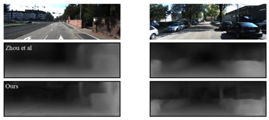
Figure 1. Example predictions by our method on KITTI dataset [16]. Compared against [5], our approach recovers more details in the scene.

The main contributions of this paper are:

• We propose a depth prediction method for AMP based on unsupervised learning, which can learn from video sequences and simultaneously estimate the depth structure of the scene and the ego-motion.
• Our method makes the spatial correspondence between pixel points consistent with the image area by smoothing the 3D corresponding vector field by 2D image. This effectively improves the depth prediction ability of the neural network.
• The model is trained and evaluated on the KITTI dataset provided by [16]. The results of the assessment indicate that our unsupervised method is superior to existing methods of the same type and has better quality than other self-supervised and supervised methods in recent years.

2. Related Work

Traditional Monocular Methods: Traditional monocular methods always use multi-view information to estimate depth of scene. Structure from motion (SfM) and simultaneous localization and mapping (SLAM) are typical ones of traditional methods. Since the depth of the object in the image cannot be directly calculated, the SLAM methods based on monocular camera need to first analyze the relationship of the position of the same points in different views, and then estimate the ego-motion and the depth of the points in the scene simultaneously for example [6,7]. Therefore, points in different views first need to be matched with each other.

In general, there are two ways to match pixels points in different views: indirect matching methods and direct matching methods [7,17]. Indirect matching, which is also known as keypoint-based methods, first extract feature points in images and calculate feature descriptors, and then match points in different views according to their descriptors [6] are typical indirect matching method. This type of method only matches hundreds of feature points in entire image, only the depth of the feature points can be estimated, dense depth information cannot be reconstructed. In contrast, direct matching, which is also known as dense-based methods, can provide dense depth map of the whole image. Refs. [18,19] are typical direct matching method. Dense-based methods first smooth the images, and then project points in source image to target image and calculate reprojection error, finally camera position and scene depth are optimized by minimizing the reprojection error. This inspired people to use geometric constraints for the training of neural networks. Dense-based method minimizes the reprojection error to optimize depth map and ego-motion, while learning-based method minimizes the reprojection error to optimize weight factor of neural networks.

CNN for Geometry Understanding: A typical CNN structure consists of convolutional layers and fully connected layers, and this structure is widely used in the fields of image recognition and target detection, for example [4], etc. [20] applied a typical CNN structure in depth prediction. However, due to the existence of fully connected layers, the 2D feature map obtained through the convolutional layers needs to be converted into a 1D feature vector of a specific length before being passed into fully connected layers. In this step the spatial relationship between the image pixels is lost and the size of the input image is limited. The fully connected layer is not suitable for dense-to-dense predictions, so fully convolutional network containing only convolutional layers and pooling layers emerges and gets applied to image segmentation in [21]. Ref. [12] improved their prior work with fully convolutional network. Ref. [22] extended the traditional deep neural network by adding a residual structure to the network, which effectively improved the training efficiency. Ref. [23] applied this residual neural network to the depth estimation of the scene.

On the basis of [20,24] combined with conditional random fields (CRFs) to jointly estimate depth and semantic segmentation information from a single image. Ref. [25] constructed a joint optimization depth network to realize the joint estimation of semantic segmentation and depth calculation [26] regarded the single image depth estimation problem as a multi class classification problem, and estimated the corresponding depth value of each pixel by training the depth neural network classifier. Ref. [27] adopted fully convolutional network and optical flow as auxiliary information to achieve depth estimation of the occluded areas in the image.Liu et al. [28] skillfully combined continuous conditional random field (CRF) with deep convolutional neural networks (DCNNs), and proposed a deep convolutional neural field to estimate depth from a single image, particularly, the method proposed by [28] applied to general scenes without any prior and extra information. Ref. [29] proposed a multi-scale depth estimation method, extract depth information and gradient information using a dual flow network and then fused to perform depth estimation.

At the same time, researchers have also explored the ability of deep learning methods to estimate the ego-motion among views. Ref. [30] proposed a method for estimating ego-motion from video images by training neural networks through LIDAR data. In their method, the LIDAR provides the depth information of the scene, thus the ego-motion can be easily guaranteed, but the LIDAR data are not easy to obtain compared to the image data. By combining the CNN network and the RNN network, Ref. [31] fused video sequence and inertial sensor (IMU) data to estimate the ego-motion. However, their work did not consider depth information of the scene.

Unsupervised Learning of Depth Estimation: The depth estimation methods based on unsupervised learning share the same kernel with the dense SLAM method, that is projecting images of different views, and calculating reprojection error as the loss function. The difference from the dense SLAM method is that the unsupervised learning methods minimize the reprojection error to optimize the parameters of the neural network, which enables the neural network to output the correct depth information.

Calculating reprojection error requires the depth structure of the scene and ego-motion. Ref. [4] proposed an auto-encoder network based on the binocular vision for depth estimation. This method predicts the depth structure from the image of a single camera and projects it to another camera to calculate the reprojection error. The binocular vision-based approach depends on the accuracy of the ego-motion. However, the binocular vision system requires complex configuration and calibration. Ref. [5] proposed a complete unsupervised depth estimation method, which predicts the depth of a single image and the ego-motion among views and calculates the reprojection error by warping nearby views to the target using the predicted depth and ego-motion, which make it possible to train the network using monocular video sequence.

Ref. [15] used stereo images as training supervision, and synthesized images by introducing left and right parallax consistency and estimating stereo parallax based on deep network;then the neural network is trained to estimate the depth of a single image by comparing the grayscale difference between the input stereo image and the composite image. Ref. [32] estimated the depth information in a single image by using two CNN modules on the basis of [15]. Ref. [33] extended the method in [15], using monocular image sequence or binocular stereo image sequence as training data and composite image as supervision data to achieve depth estimation. Rezende et al. [34,35] used encoder-decoder architecture of 3D CNN to achieve 3D reconstruction of single image, the former infers the three-dimensional model of the scene directly from the two-dimensional image in the way of probability reasoning, and uses the three-dimensional model as the supervision to train; the latter, according to the given perspective, renders the corresponding projected images from the 3D model generated by the deep network as additional supervision to train the network. Ref. [36] used monocular image sequences as training data and predicted depth, posture, semantic segmentation and other information according to the depth estimation neural network module, attitude estimation neural network module and image segmentation neural network module. Ref. [37] proposed GeoNet, a network framework used to learn monocular depth, video motion estimation and optical flow information, which effectively solved the problems of image occlusion and texture blurring. Ref. [38] presented the first learning based approach for estimating depth from dual-pixel cues. In order to solve the limitation of monocular depth estimation algorithm due to the lack of high-quality datasets, Ref. [38] captured a large dataset of in-the-wild five-viewpoint RGB images paired with corresponding dual-pixel data.

Because of the similarity between the unsupervised learning methods and the dense SLAM methods, problems in the dense SLAM methods are also reflected in the unsupervised deep learning methods. Due to geometric constraints, the monocular SLAM methods cannot estimate the real scale of the scene. In unsupervised learning methods, a smaller inverse depth scale always results in smaller loss value, which makes predicted depth continue to shrink as the training process approaches until it approaches zero and hinders the converge of the training result process. Ref. [39] effectively suppressed the reduction of the output by normalizing the inverse depth of the output. However, their methods still have poor performance in thin structure and the detail quality of the depth map. In this paper, we improve the typical unsupervised method by involving a loss function based on pixel corresponding consistency, which makes our networks recover more detail of depth information and improves the depth estimation results in thin structure regions.

3. The Proposed Approach

This paper proposes an unsupervised learning depth estimation method based on 3D-2D consistency, which is used to train a neural network to estimate the depth of a scene. First, the image is divided into the original image used to estimate the depth and the target image used to build the loss. The relationship between the depth of the original image and the motion of the camera is estimated through the neural network. Then the projected image of the original image is constructed by the projection transformation, and the reconstruction loss is calculated. At the same time, the 3D scene flow was constructed according to the depth and motion relations, and the 3D-2D consistency loss was calculated. Finally, the neural network was trained by minimizing the loss function.

3.1. Differentiable Reprojection Error

In our method, we train the neural network by minimizing the re-projection loss. The re-projection loss refers to the loss between the point of the projected target image.

Inspired by [5], for the rigid part of image, we use depth and camera pose to calculate the loss. For two frames $I_{t-1}$ and $I_t$ in a sequence of images, $I_{t-1}$ is the source view and $I_t$ is the target view. Our method can reconstruct the target view $I_t$ by sampling pixels from a source view $I_{t-1}$ based on the predicted depth map $D_t$ and the relative pose $T_{t\to t-1}$. Let $p_t$ denote the homogeneous coordinates of a pixel in the target view, We can obtain $p_t^{\prime }s$ projected coordinates onto the source view $p_{t-1}$ as:

$$\begin{array}{c}\hfill p_{t-1}\sim K{T}_{t\to t-1}{D}_t\left(p_t\right)K^{-1}{p}_t\end{array}$$

(1)

in which K is the camera intrinsic matrix obtained by camera calibration.

Since $p_{t-1}$ is a continuous value, we use a differential bilinear sampling method to calculate discrete pixel coordinates. That is, interpolation is performed according to four pixel points (upper left, lower left, upper right, lower right) adjacent to $p_{t-1}$ to approximate [5]. Finally, the re-projection loss can be expressed as follows:

$$\begin{array}{c}\hfill L_{reproject}=\sum _p\left|I_t\left(p\right)-{\widehat{I}}_t\left(p\right)\right|\end{array}$$

(2)

in which ${\widehat{I}}_t$ denotes warped target image, p denotes pixel index.

3.2. Image Reconstruction Loss

According to the image re-projection loss, we use three pictures in the video sequence to calculate the image reconstruction loss. The gradient of the image may be unevenly distributed. To avoid this, a Gaussian smoothing is used. We complete Gaussian smoothing by convolution calculation, and its convolution kernel can be calculated as following:

$$\begin{array}{c}\hfill G(u,v)=\frac{1}{2\pi {\sigma }^2}{e}^{-(u^2+v^2)/\left(2{\sigma }^2\right)}\end{array}$$

(3)

in which u and v denotes the size of convolution kernel, $\sigma$ denotes the smooth parameters for the Gaussian.

In addition, for rigid part of the depth map is normalize by dividing by its mean, which is denoted by operator $\eta (·)$:

$$\begin{array}{c}\hfill \eta \left(d_i\right)=\frac{N{d}_i}{{\sum }_{j=1}^N{d}_j}\end{array}$$

(4)

The structural similarity (SSIM) proposed in [40] is a common metric used to evaluate the quality of image predictions. It measures the similarity between two images. SSIM is calculated as follows:

$$\begin{array}{c}\hfill SSIM(x,y)=\frac{(2{\mu }_x{\mu }_y+c_1)(2{\sigma }_{xy}+c_2)}{({\mu }_x^2+{\mu }_y^2+c_1)({\sigma }_x+{\sigma }_y+c_2)}\end{array}$$

(5)

in which $\mu$ and $\sigma$ denote the mean and the variance, respectively, $c_1$ and $c_2$ are the constant used to maintain stability. We calculate $\mu$ and $\sigma$ by pooling using the method proposed by [14]. Since SSIM needs to be maximized and the upper bound is 1, the SSIM loss is designed as:

$$\begin{array}{c}\hfill L_{SSIM}=\sum _p\left[1-SSIM(I_t^p,{\widehat{I}}_t^p)\right]M_{t-1}^p\\ \hfill +\sum _p\left[1-SSIM(I_t^p,{\widehat{I}}_t^p)\right]M_{t+1}^p\end{array}$$

(6)

in which $M_{t-1}^p$ and $M_{t+1}^p$ denote the masks calculated through neural network and represent the legal part of projected images $I_{t-1}$ and $I_{t+1}$, respectively. Then, the image reconstruction loss $L_{recon}$ can be expressed as:

$$\begin{array}{c}\hfill L_{recon}=S(\zeta \left(I_s\left(p_t\right)\right),I_t\left(\left[K|0\right]T_{t\to s}\left[\begin{array}{c}{D}_t\left(p_t\right)K^{-1}{p}_t\\ 1\end{array}\right]\right))\end{array}$$

(7)

in which $\zeta$ denotes the Gaussian smooth process and S is the combination of abs error and SSIM error.

3.3. Corresponding Consistency Loss

As can be seen from the previous section, in the process of image pixel correspondence, the image reconstruction loss only depends on the pixel difference of the independent pixel points, so the regional relationship of the pixel points is not considered. In addition, for weak texture regions, the color of pixels in a certain range is almost the same, and the corresponding pixel points do not produce effective errors so that the loss function cannot be effectively calculated. In the traditional dense SLAM method, there are two main ways to solve this problem. One way is to increase the length of the input sequence, so that the pixel points correspond in a larger range. A typical example is [18], the system inputs multiple images and builds cost volumes so that pixel points can be matched among several different views to find the best correspondence. The other is to remove weak texture parts in the image by checking the gradient of the image. Before matching the pixel points, these methods calculate image pixel gradient and remove the areas with low pixel gradient. Only the remaining area with a high pixel gradient is matched. A typical example is [19]. The above two methods cannot be applied to neural-network-based methods for these reasons. For methods similar to [18], increasing the length of the input sequence will increase the input size of the network, resulting in unstable ego-motion estimation. For methods similar to [19], removing the area with a low pixel gradient will make the network not able to gather necessary information thus affect the converge. Therefore, a new loss function must be designed according to the correspondence between pixel points after image reprojection.

The correspondence between pixel points can be expressed in the form of a vector field, which is the form of optical flow for a 2D image, that is, the movement of a point from the first frame image to the second frame image in the x-axis and y-axis directions. For example, Figure 2 is an optical flow image and its vector field representation. In general, we assume that the 2D optical flow has a similar gradient with the image, and smoothing the corresponding vector field will enhance this consistency.

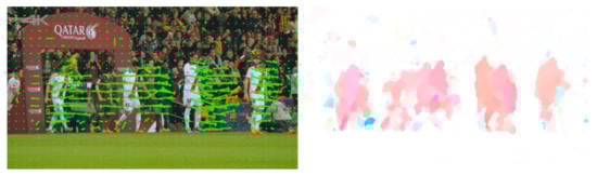
Figure 2. The optical flow field shown in image and its vector field representation [41].

However, the above assumption is valid only in the case where the pixel points only have planar motion. Due to the spatial relationship of the scene, the closer the object is to the camera, the more there are the position changes on the image when the camera moves. Therefore, it is necessary to calculate a 3D corresponding vector field of the pixel points in the image and smooth the 3D vector field according to the 2D image.

The method is to first calculate the 3D corresponding field of the target image, and then smooth it according to the image pixels gradient. As shown in Figure 3, for pixel point $p_{ij}={\left[i,j,1\right]}^T$ in the image, and its spatial coordinate q can be obtained according to the depth D as follow:

$$\begin{array}{c}\hfill q_{ij}=D\left(p\right)K^{-1}{\left[i,j,1\right]}^T\end{array}$$

(8)

in which K denotes the camera intrinsic matrix. $T_{t->t-1}$ is the ego-motion from target view to source view, then the spatial position motion of the point can be expressed as:

$$\begin{array}{c}\hfill s_{ij}=(1-T_{t\sim t-1})D\left(p\right)K^{-1}{\left[i,j,1\right]}^T\end{array}$$

(9)

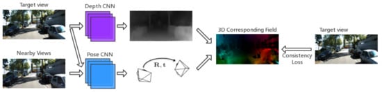
Figure 3. Calculation of consistency loss. The depth map of the target view and the ego-motion are estimated by CNN network, respectively. The 3D corresponding field of target view is calculated based on the depth information and the ego-motion. After that we smooth the 3D field according to pixel gradient of target view.

According to the above formula, the 3D corresponding field S of the pixel of the entire image can be calculated. Smoothing S according to the image pixel gradient can make the spatial motion of points consistent with the image gradient. The spatial corresponding consistency loss $L_{consist}$ can be designed as:

$$\begin{array}{c}\hfill L_{consist}=\sum _{ij}\left|\left|{\partial }_x{S}^{ij}\right|\right|e^{-\left|\left|{\partial }_x{I}^{ij}\right|\right|}\\ \hfill +\sum _{ij}\left|\left|{\partial }_y{S}^{ij}\right|\right|e^{-\left|\left|{\partial }_y{I}^{ij}\right|\right|}\end{array}$$

(10)

in which I denotes the source image and S denotes the 3D corresponding vector field, i and j are the pixel indexes and x and y are the image coordinate axis directions. This approach ensures that the spatial motion of the pixels is consistent with the image gradient change.

3.4. Learning Setup

All loss functions are applied to four different scales s, from the original resolution of the image to 1/8 of image resolution in width and height. The total loss function can be expressed as:

$$\begin{array}{c}\hfill L=\sum _s(\alpha L_{rec}^s+\beta L_{consist}^s+\gamma L_{sm}^s+\omega L_{SSIM}^s)\end{array}$$

(11)

in which $\alpha ,\beta ,\gamma ,\omega$ are weight parameters. $L_{sm}^s$ [5] is a depth smoothness loss is also employed to regularize the depth estimates. We use TensorFlow framework proposed in [42] to build our neural network structure and Adam optimizer [43]. Neural network training typically converges after 150 K iterations. During training, we scaled the image to the resolution of 128 × 416, but due to the full convolution structure, both the depth estimation network and the ego-motion estimation network can input images of any size during testing.

4. Experiments and Discussion

In this section, we first introduce the network structure of our model, and its training details of it. Then we introduce the datasets and compare the performance of our method with other similar methods.

4.1. Network Structure

There were two sub-nets in our framework: the depth estimation network and the ego-motion estimation network. The depth estimation network predicated one-channel depth map of four different scales from a single three-channel image while the ego-motion estimation network predicated six-DOF of ego-motion from three consecutive images.

The depth estimation network was based on the [44] network structure, that is also adopted by [5]. As show in Figure 4, this network structure could be divided into encoder part and decoder part, adding a skip structure and adopting an output of four scales. The overall network structure is shown in Table 1. Since the full convolutional neural network did not restrict the size of the input image, the two columns of the table, input size and output size, indicate the ratio of the image edge length to the original image. Except for the predicted output layer, each convolutional layer was activated by the RELU activation function. Since the inverse depth result of the output was not conducive to network calculation, we multiplied the output by 10 to control it within the appropriate range and added 0.01 to prevent the error caused by little values.

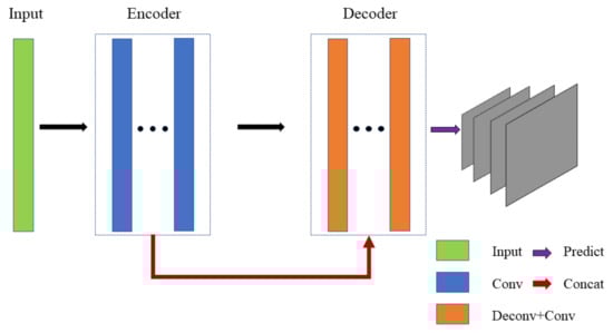
Figure 4. Depth estimation network structure The network structure is based on encoder-decoder architecture, including 28 layers, with a skip structure. The network provides output results at four scales for calculating losses at different resolutions.

Table 1. The depth estimation network structure.

Name	Kernel Size	Stride	Output Channel	Input Size	Output Size	Input
conv1a	$7\times 7$	2	32	1	$1/2$	image
conv1b	$7\times 7$	1	32	$1/2$	$1/2$	conv1a
conv2a	$5\times 5$	2	64	$1/2$	$1/4$	conv1b
conv2b	$5\times 5$	1	64	$1/4$	$1/4$	conv2a
conv3a	$3\times 3$	2	128	$1/4$	$1/8$	conv2b
conv3b	$3\times 3$	1	128	$1/8$	$1/8$	conv3a
conv4a	$3\times 3$	2	256	$1/8$	$1/16$	conv3b
conv4b	$3\times 3$	1	256	$1/16$	$1/16$	conv4a
conv5a	$3\times 3$	2	512	$1/16$	$1/32$	conv4b
conv5b	$3\times 3$	1	512	$1/32$	$1/32$	conv5a
conv6a	$3\times 3$	2	512	$1/32$	$1/64$	conv5b
conv6b	$3\times 3$	1	512	$1/64$	$1/64$	conv6a
conv7a	$3\times 3$	2	512	$1/64$	$1/128$	conv6b
conv7b	$3\times 3$	1	512	$1/128$	$1/128$	conv7a
upcnv7	$3\times 3$	2	512	$1/128$	$1/64$	conv7b
icnv7	$3\times 3$	1	512	$1/64$	$1/64$	upcnv7 + conv6b
upcnv6	$3\times 3$	2	512	$1/64$	$1/32$	icnv7
icnv6	$3\times 3$	1	512	$1/32$	$1/32$	upcnv6 + conv5b
upcnv5	$3\times 3$	2	256	$1/32$	$1/16$	icnv6
icnv5	$3\times 3$	1	256	$1/16$	$1/16$	upcnv5 + conv4b
upcnv4	$3\times 3$	2	128	$1/16$	$1/8$	icnv5
icnv4	$3\times 3$	1	128	$1/8$	$1/8$	upcnv4 + conv3b
pred4	$3\times 3$	1	1	$1/8$	$1/8$	icnv4
upcnv3	$3\times 3$	2	64	$1/8$	$1/4$	icnv4
icnv3	$3\times 3$	1	64	$1/4$	$1/4$	upcnv3 + conv2b + pred4up
pred3	$3\times 3$	1	1	$1/4$	$1/4$	icnv3
upcnv2	$3\times 3$	2	32	$1/4$	$1/2$	icnv3
icnv2	$3\times 3$	1	32	$1/2$	$1/2$	upcnv2 + conv1b + pred3up
pred2	$3\times 3$	1	1	$1/2$	$1/2$	icnv2
upcnv1	$3\times 3$	2	16	$1/2$	1	icnv2
icnv1	$3\times 3$	1	16	1	1	upcnv1 + pred2up
pred1	$3\times 3$	1	1	1	1	icnv1

The encoder included 14 layers, all of which were convolutional layers. The output size of every two layers was the same, divided into a group. The input of the first group (conv1a and conv1b) was the original image, the size of the convolution kernel was 7 × 7, and the output size was a feature map of 1/2 of the original image. Each subsequent group was similar to the first group, and the output size of the previous group was 1/2 of the input feature map.The dimension of the feature graph increased with the depth of the network and finally reached 512.

The decoder was complex, including convolutional layer and deconvolutional layer. Like the encoder, the decoder was divided into a group with the same output size every two layers. The first group consisted of upconv7 and icnv7 layers. upconv7 was the reverse convolution layer. Unlike convolution layer, the deconvolution layer enlarged the feature map and output the result with the output size of twice the input. icnv7 was the convolutional layer, and the input contained skip structure, i.e., the upconv7 was superimposed with the conv6b in the encoder as the input, thus preserving the detailed features of the shallow layers. The second group (upconv6 and icnv6) and the third group (upconv5 and icnv5) were similar in structure to the first group. After one group, the feature map size was doubled. The fourth group was different from the first three groups by adding the output layer pred4, which output the estimation result of one dimension. The overall structure of the fifth group was similar to that of the fourth group, while the skip structure was more complicated. The skip structure of the convolutional layer icnv3 superimposed upconv3 and conv2b, and at the same time enlarged the output result of pred4 to pred4up and superimposed it, while ensuring that the deep global information and the shallow detail information were preserved. The sixth group (upconv2, icnv2 and pred2) had the same structure as the fifth group. In the seventh group (upconv1, icnv1 and pred1) structure, because there was no feature layer with the same size as the original image, the skip structure of the convolution layer iconv1 superimposed upconv1 with the result pred2up of the previous layer’s estimation.

The depth estimation network structure did not include a fully connected layer and a pooling layer. The disadvantage of the fully connected layer was that the fixed feature vector length limited the input size, and the transformation of the feature vector lost the spatial characteristics of the pixel. In traditional convolutional neural networks, the pooling layer is used for downsampling, so information loss will occur. The direct use of a convolutional layer with a step size of 2 to achieve downsampling circumvented this problem.

The ego-motion estimation network had the same network structure used in [5]. As show in Figure 5. The network input several continuous images in the image sequence, output six-DOF camera motion, and output masks of four scales corresponding to the depth map, which were used to exclude the non-rigid body parts in the scene. In the ego-motion vector, the position change part was divided by the average of depth, so that the motion of the camera corresponded to the scale of the depth map.

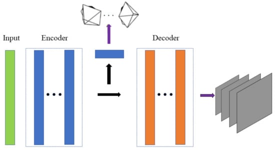
Figure 5. Ego-motion estimation network: the network structure is designed based on the encoder-decoder architecture. The encoder contains 5 layers, all of which are convolutional layers, for extracting image features. The specific structure is shown in Table 2.

The camera motion estimation part of the network was dense to sparse estimation, so the deconvolution layer was not adopted and only contained three convolution layers. The structure is shown in Table 3, where N is the number of target images in the image sequence. The mask estimation part of the network was dense to dense estimation, which contained only five deconvolution layers and four output layers. The structure is shown in Table 4, where N is the number of target images in the image sequence.

Table 3. Camera moving part structure of ego-motion estimation network.

Name	Kernel Size	Stride	Output Channel	Input
conv6	$3\times 3$	2	256	conv5
conv7	$3\times 3$	2	265	conv6
conv8	$3\times 1$	1	$6\times N$	conv7

Table 4. Mask estimation of partial structure of ego-motion estimation network.

Name	Kernel Size	Stride	Output Channel	Input Size	Output Size	Input
upcnv5	$3\times 3$	2	256	$32/1$	$1/16$	conv5
upcnv4	$3\times 3$	2	128	$1/16$	$1/8$	upcnv5
mask4	$3\times 3$	1	$2\times N$	$1/8$	$1/8$	upcnv4
upcnv3	$3\times 3$	2	64	$1/8$	$1/4$	upcnv4
mask3	$3\times 3$	1	$2\times N$	$1/4$	$1/4$	upcnv3
upcnv2	$3\times 3$	2	32	$1/4$	$1/2$	upcnv3
mask2	$3\times 3$	1	$2\times N$	$1/2$	$1/2$	upcnv2
upcnv1	$3\times 3$	2	16	$1/2$	1	upcnv2
mask1	$3\times 3$	1	$2\times N$	1	1	upcnv1

4.2. Datasets Description

In the experiments, three widely used depth estimation datasets were used to test the proposed approach: KITTI, Apolloscape [45] and Cityscapes [46].

KITTI dataset was the largest data set for evaluating computer vision algorithms in autonomous driving scenarios in the world. It collected 61 scenes including rural areas and urban highways with optical lenses, cameras, LIDAR and other hardware equipment. There were at most 30 pedestrians and 15 cars in the image, and there were different degrees of occlusion. The normal RGB image resolution in KITTI was 375 × 1242 and the ground-truth depth resolution was 228 × 912. The original KITTI dataset did not have a true depth map, but contained sparse 3D laser measurements captured with the Velodyne laser sensor. To be able to evaluate in the KITTI dataset, we needed to map the laser measurements into the graph space to generate the ground-truth depth corresponding to the original image.

The Cityscapes dataset, jointly provided by three German companies, including Daimler, contains stereo vision data for more than 50 cities, with higher resolution and quality images. It contained a rich and distinct set of scenes from KITTI. Compared to the KITTI dataset, the images from the Cityscapes dataset were of better quality, with more diverse shooting scenes and higher resolution.

Apolloscape dataset was provided by the company, including perception, the simulation scene, road network data, such as hundreds of frames per-pixel semantic segmentation of high-resolution image data, as well as the corresponding per-pixel semantic annotation, dense point cloud, three-dimensional images, three-dimensional panoramic images, and further more complex environment, weather and traffic conditions, etc.

4.3. Experiment Settings

In this paper, the KITTI2012 dataset [16] was used to train the neural network. In the training, the resolution of the image was set to $416\times 128$. Since the network structure is full convolutional, the image of any size can be used in the actual test. In this paper, TensorFlow [42] was used to build a neural network, and the Adam [43] optimizer was used. The learning rate was set to 0.001, and the training process usually converged after about 150 K iterations.

For the evaluation of depth results, this paper used the same indicators and test set partitioning as [12]. This division included 700 images from the KITTI test dataset (this division excludes visually similar images). During the assessment, the effective distances were set to 50 m and 80 m, respectively, and each method was evaluated using the error used in [12].

The evaluation criteria included Absolute Relative error (Abs Rel), Square Relative error (Sq Rel), Root Mean Squared Error (RMSE) and Root Mean Squared logarithmic Error (RMSE log). For the absolute relative error and square relative error, this paper adopted the calculation method in [20]. For RMSE, it could be calculated by the following formula:

$$\begin{array}{c}\hfill RMSE=\sqrt{\frac{1}{n}\sum _{i=1}^n{(y_i-{\widehat{y}}_i)}^2)}\end{array}$$

(12)

where, n is the total number of pixels, and $y_i$ and ${\widehat{y}}_i$ are the actual and estimated depths, respectively. RMSE log could be calculated according to the following formula:

$$\begin{array}{c}\hfill RMSElog=\sqrt{\frac{1}{n}\sum _{i=1}^n{(log(y_i+1)-log({\widehat{y}}_i+1))}^2)}\end{array}$$

(13)

The parameters were the same as Formula (12).

For camera position estimation, two sequences Seq.09 and Seq.10 in KITTI dataset were used in this paper. The evaluation index was Absolute Trajectory Error (ATE), which could be calculated according to the following formula:

$$\begin{array}{c}\hfill ATE=Q^{-1}SP\end{array}$$

(14)

where $Q\in SE\left(3\right)$ is the actual pose of the camera, $P\in SE\left(3\right)$ is the estimated camera pose, and $S\in Sim\left(3\right)$ is the similar transformation matrix from the estimated pose to the actual pose.

4.4. Comparisons with Other Methods

To demonstrate the superiority of our method, we compared it with some classical methods, including supervised methods [13,20] and unsupervised methods [4,5]. The ground-truth depth was from LIDAR data, which were obtained by projecting the point cloud to the image plane.

4.4.1. Evaluation of Depth Estimation

Table 5 compares the results of our work with existing work in estimating the depth of the scene. As seen in Table 5, “Ours” and “Ours consis” indicate the results of using and not using the consistency constraints, respectively. Experimental results showed that our method was significantly better than supervised learning methods, which showed that our method overcame the impact of the supervised learning method on the results due to the poor quality of the supervised data. Compared with the benchmark work [5], our results reduced the average error from 0.208 to 0.169, which reflected the effectiveness of our method. Our results still had some gaps with the results of the stat-of-the-art method of 0.148 by Godard [15] since their method used images with known camera baseline as supervised data, we believe that the gap is due to our method not further constraining the ego-motion. In addition, the consistency loss further narrowed the error from 0.176 to 0.169, which reflected the effect of our loss term. Figure 6 is a qualitative comparison of visualizations. The experimental results reflected the ability of our method to understand 3D scenes, that is, the method successfully analyzed the 3D consistency of different scenes.

Table 5. Depth evaluation results for the KITTI test set, K indicates training on KITTI, and C indicates training on Cityscapes [46]. Ours indicates that the consistency loss is not used, and Ours consis indicates the result using the consistency loss term.

Method	Cap	Dataset	Supervised		Error				Accuracy Metric
			Depth	Pose	Abs Rel	Sq Rel	RMSE	RMSE log	$\mathit{\delta }<1.25$	$\mathit{\delta }<1.{25}^2$	$\mathit{\delta }<1.{25}^3$
Eigen et al. [20] Coarse	80	K	√		0.214	1.605	6.563	0.292	0.673	0.884	0.957
Eigen et al. [20] Fine	80	K	√		0.203	1.548	6.307	0.282	0.702	0.890	0.958
Liu et al. [13]	80	K	√		0.202	1.614	6.307	0.282	0.678	0.895	0.965
Zhou et al. [5]	80	K			0.208	1.768	6.856	0.283	0.678	0.885	0.957
Zhou et al. [5]	80	K + C			0.183	1.595	6.720	0.270	0.733	0.901	0.959
Ours	80	K			0.176	1.497	6.898	0.274	0.739	0.898	0.956
Ours consis	80	K			0.169	1.387	6.670	0.265	0.748	0.904	0.960
Garg et al. [4]	50	K		√	0.169	1.080	5.104	0.273	0.740	0.904	0.962
Zhou et al. [5]	50	K + C			0.173	1.151	4.990	0.250	0.751	0.915	0.969
Ours	50	K			0.167	1.116	4.940	0.249	0.760	0.917	0.967
Ours consis	50	K			0.162	1.039	4.851	0.244	0.767	0.920	0.969

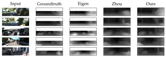
Figure 6. Qualitative results on KITTI [16] test set. Our method captures details in thin structures and preserves consistently high-quality predictions both in close and distant regions.

4.4.2. Evaluation of Ego-Motion

During the training, the result of motion estimation greatly affected the accuracy of depth estimation. In order to evaluate the accuracy of our method in camera motion estimation, we conducted an experiment on the KITTI odometry split dataset. This data set contained 11 video sequences and their corresponding sensor information which are obtained through IMU/GPS. We used the sequence 00–08 to train the model, and the sequence 09–10 to evaluate it. Additionally, we compared our method with a typical visual odometry of ORB-SLAM [6]. ORB-SLAM is an indirect SLAM method which calculates camera motion and scene depth through feature point matching. It has a bundle adjustment back-end based on graph optimization, which further constrains ego-motion by non-adjacent images. Therefore, we compared our approach to two different SLAM processes: (1) “ORB-SLAM (short)” containing only five frames as input, which had no graph optimization; (2) “ORB-SLAM (full)” containing the entire process and all frames. As shown in Table 6, we compared our method with existing work on ego-motion estimation. Our method outperformed other unsupervised learning methods, approaching the ORB-SLAM with global optimization.

Table 6. Absolute Track Error (ATE) tested on the KITTI odometry dataset [16]. Ours indicates that the consistency loss is not used, and Ours consis indicates the result using the consistency loss term.

Method	Seq.09	Seq.10
ORB-SLAM [6] (Full)	0.014 ± 0.008	0.012 ± 0.011
ORB-SLAM [6] (Short)	0.064 ± 0.141	0.064 ± 0.130
Mean SLAM	0.032 ± 0.026	0.028 ± 0.023
Zhou et al. [5]	0.021 ± 0.017	0.020 ± 0.015
Ours	0.017 ± 0.015	0.016 ± 0.012
Ours consis	0.015 ± 0.013	0.014 ± 0.012

4.4.3. Depth Results on Apollo and Cityscapes

To prove the versatility of our method, we directly applied our model trained on KITTI to the Apollo stereo test set [45] and Cityscapes test set. Our model could still output accurate prediction results, even if the scene structure was more complex. As shown in Figure 7 and Figure 8, our method could recover more details.

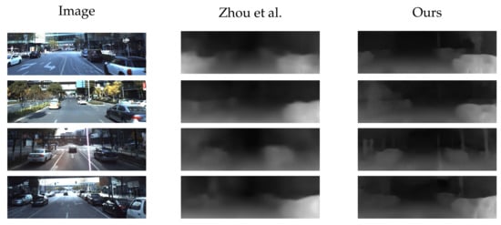
Figure 7. Example predictions by our method on Apollo dataset [45]. The model is only trained on KITTI dataset but also performs well in other cases. Compared with [5], our method recovers more details.

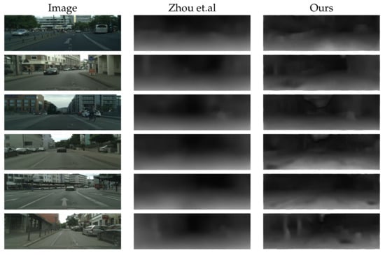
Figure 8. Example predictions by our method on Cityscapes dataset [46]. Our method can predict high quality depth information from a single image, even in areas where the laser scanning system cannot measure very well.

5. Conclusions

We improve the existing unsupervised learning depth estimation method by enhancing the consistency between the 3D corresponding vector field and the 2D image. It effectively improves the prediction result and exceeds similar existing methods. The experiments on the KITTI dataset demonstrated that our method exceeded the previous unsupervised learning methods and supervised learning methods. The results on the Apolloscape and Cityscapes datasets demonstrate the strong generality of our proposed approach.

Compared with the latest methods involved flow prediction, our method only predicts the camera position change and the scene depth structure and does not involve the prediction of the image flow, so the performance can only be close to it. Recent studies have demonstrated the ability of deep neural networks in the field of depth estimation and flow estimation. This also represents a great potential for deep learning methods to solve the problem of moving object depth and spatial motion in estimated scenes.

References

- Wymeersch, H.; Seco-Granados, G.; Destino, G.; Dardari, D.; Tufvesson, F. 5G mmWave positioning for vehicular networks. IEEE Wirel. Commun. 2017, 24, 80–86. [Google Scholar] [CrossRef]
- Lu, Z.; Huang, Y.C.; Bangjun, C. A Study for Application in Vehicle Networking and Driverless Driving. In Proceedings of the 2019 3rd International Conference on Computer Science and Artificial Intelligence, Beijing, China, 6–8 December 2019; pp. 264–267. [Google Scholar]
- Zhao, Y.; Jin, F.; Wang, M.; Wang, S. Knowledge Graphs Meet Geometry for Semi-supervised Monocular Depth Estimation. In Proceedings of the International Conference on Knowledge Science, Engineering and Management, Hangzhou, China, 28–30 August 2020; pp. 40–52. [Google Scholar]
- Garg, R.; Kumar, B.G.V.; Carneiro, G.; Reid, I.D. Unsupervised CNN for Single View Depth Estimation: Geometry to the Rescue. In Proceedings of the European Conference on Computer Vision, Amsterdam, The Netherlands, 8–16 October 2016; pp. 740–756. [Google Scholar]
- Zhou, T.; Brown, M.; Snavely, N.; Lowe, D.G. Unsupervised Learning of Depth and Ego-Motion from Video. In Proceedings of the Computer Vision and Pattern Recognition, Honolulu, HI, USA, 21–26 July 2017; pp. 6612–6619. [Google Scholar]
- Murartal, R.; Montiel, J.M.M.; Tardos, J.D. ORB-SLAM: A Versatile and Accurate Monocular SLAM System. IEEE Trans. Robot. 2015, 31, 1147–1163. [Google Scholar] [CrossRef]
- Engel, J.; Koltun, V.; Cremers, D. Direct Sparse Odometry. IEEE Trans. Pattern Anal. Mach. Intell. 2018, 40, 611–625. [Google Scholar] [CrossRef] [PubMed]
- Wang, J.; Liu, Z.; Xie, R.; Ran, L. Radar HRRP Target Recognition Based on Dynamic Learning with Limited Training Data. Remote Sens. 2021, 13, 750. [Google Scholar] [CrossRef]
- Kazimierski, W.; Zaniewicz, G. Determination of Process Noise for Underwater Target Tracking with Forward Looking Sonar. Remote Sens. 2021, 13, 1014. [Google Scholar] [CrossRef]
- Li, B.; Gan, Z.; Chen, D.; Sergey Aleksandrovich, D. UAV Maneuvering Target Tracking in Uncertain Environments Based on Deep Reinforcement Learning and Meta-Learning. Remote Sens. 2020, 12, 3789. [Google Scholar] [CrossRef]
- Guo, J.; Bai, C.; Guo, S. A Review of Monocular Depth Estimation Based on Deep Learning. Unmanned Syst. Technol. 2019, 3. Available online: https://kns.cnki.net/kcms/detail/detail.aspx?dbcode=CJFD&dbname=CJFDLAST2019&filename=UMST201902003&v=LxXxs2LYM%25mmd2FrpCJsoTtiaExYvBg0cRUvrHeXluBqPeql%25mmd2FO67HDuhfchKopV1yVha7 (accessed on 10 March 2021).
- Eigen, D.; Fergus, R. Predicting Depth, Surface Normals and Semantic Labels with a Common Multi-scale Convolutional Architecture. In Proceedings of the International Conference on Computer Vision, Santiago, Chile, 13–16 December 2015; pp. 2650–2658. [Google Scholar]
- Liu, F.; Shen, C.; Lin, G.; Reid, I. Learning Depth from Single Monocular Images Using Deep Convolutional Neural Fields. IEEE Trans. Pattern Anal. Mach. Intell. 2016, 38, 2024–2039. [Google Scholar] [CrossRef] [PubMed]
- Mahjourian, R.; Wicke, M.; Angelova, A. Unsupervised Learning of Depth and Ego-Motion from Monocular Video Using 3D Geometric Constraints. In Proceedings of the Computer Vision and Pattern Recognition, Salt Lake City, UT, USA, 18–23 June 2018; pp. 5667–5675. [Google Scholar]
- Godard, C.; Aodha, O.M.; Brostow, G.J. Unsupervised Monocular Depth Estimation with Left-Right Consistency. In Proceedings of the Computer Vision and Pattern Recognition, Honolulu, HI, USA, 21–26 July 2017; pp. 6602–6611. [Google Scholar]
- Geiger, A. Are we ready for autonomous driving? The KITTI vision benchmark suite. In Proceedings of the 2012 IEEE Conference on Computer Vision and Pattern Recognition (CVPR), Providence, RI, USA, 16–21 June 2012. [Google Scholar]
- Taketomi, T.; Uchiyama, H.; Ikeda, S. Visual SLAM algorithms: A survey from 2010 to 2016. IPSJ Trans. Comput. Vis. Appl. 2017, 9, 16. [Google Scholar] [CrossRef]
- Newcombe, R.A.; Lovegrove, S.J.; Davison, A.J. DTAM: Dense tracking and mapping in real-time. In Proceedings of the IEEE International Conference on Computer Vision, ICCV 2011, Barcelona, Spain, 6–13 November 2011. [Google Scholar]
- Engel, J.; Schöps, T.; Cremers, D. LSD-SLAM: Large-Scale Direct Monocular SLAM. In Proceedings of the European Conference on Computer Vision, Zurich, Switzerland, 6–12 September 2014. [Google Scholar]
- Eigen, D.; Puhrsch, C.; Fergus, R. Depth map prediction from a single image using a multi-scale deep network. In Proceedings of the Advances in Neural Information Processing Systems, Montreal, QC, Canada, 8–13 December 2014; pp. 2366–2374. [Google Scholar]
- Long, J.; Shelhamer, E.; Darrell, T. Fully convolutional networks for semantic segmentation. In Proceedings of the Computer Vision and Pattern Recognition, Boston, MA, USA, 7–12 June 2015; pp. 3431–3440. [Google Scholar]
- He, K.; Zhang, X.; Ren, S.; Sun, J. Deep Residual Learning for Image Recognition. In Proceedings of the Computer Vision and Pattern Recognition, Las Vegas, NV, USA, 27–30 June 2016; pp. 770–778. [Google Scholar]
- Laina, I.; Rupprecht, C.; Belagiannis, V.; Tombari, F.; Navab, N. Deeper Depth Prediction with Fully Convolutional Residual Networks. In Proceedings of the International Conference on 3D Vision, Stanford, CA, USA, 25–28 October 2016; pp. 239–248. [Google Scholar]
- Wang, P.; Shen, X.; Lin, Z.; Cohen, S.; Price, B.; Yuille, A.L. Towards unified depth and semantic prediction from a single image. In Proceedings of the IEEE Conference on Computer Vision and Pattern Recognition, Boston, MA, USA, 7–12 June 2015; pp. 2800–2809. [Google Scholar]
- Jafari, O.H.; Groth, O.; Kirillov, A.; Yang, M.Y.; Rother, C. Analyzing modular CNN architectures for joint depth prediction and semantic segmentation. In Proceedings of the 2017 IEEE International Conference on Robotics and Automation (ICRA), Singapore, 29 May–3 June 2017; pp. 4620–4627. [Google Scholar]
- Fu, H.; Gong, M.; Wang, C.; Batmanghelich, K.; Tao, D. Deep ordinal regression network for monocular depth estimation. In Proceedings of the IEEE Conference on Computer Vision and Pattern Recognition, Salt Lake City, UT, USA, 18–22 June 2018; pp. 2002–2011. [Google Scholar]
- Mancini, M.; Costante, G.; Valigi, P.; Ciarfuglia, T.A. Fast robust monocular depth estimation for obstacle detection with fully convolutional networks. In Proceedings of the 2016 IEEE/RSJ International Conference on Intelligent Robots and Systems (IROS), Daejeon, Korea, 9–14 October 2016; pp. 4296–4303. [Google Scholar]
- Liu, F.; Shen, C.; Lin, G. Deep convolutional neural fields for depth estimation from a single image. In Proceedings of the IEEE Conference on Computer Vision and Pattern Recognition, Boston, MA, USA, 7–12 June 2015; pp. 5162–5170. [Google Scholar]
- Li, J.; Klein, R.; Yao, A. A two-streamed network for estimating fine-scaled depth maps from single rgb images. In Proceedings of the IEEE International Conference on Computer Vision, Venice, Italy, 22–29 October 2017; pp. 3372–3380. [Google Scholar]
- Oliveira, G.L.; Radwan, N.; Burgard, W.; Brox, T. Topometric localization with deep learning. In Robotics Research; Springer: Berlin/Heidelberg, Germany, 2020; pp. 505–520. [Google Scholar]
- Clark, R.; Wang, S.; Wen, H.; Markham, A.; Trigoni, N. VINet: Visual-Inertial Odometry as a Sequence-to-Sequence Learning Problem. In Proceedings of the National Conference on Artificial Intelligence, San Francisco, CA, USA, 4–9 February 2017; pp. 3995–4001. [Google Scholar]
- Repala, V.K.; Dubey, S.R. Dual cnn models for unsupervised monocular depth estimation. In Proceedings of the International Conference on Pattern Recognition and Machine Intelligence, Tezpur, India, 17–20 December 2019; pp. 209–217. [Google Scholar]
- Godard, C.; Mac Aodha, O.; Firman, M.; Brostow, G.J. Digging into self-supervised monocular depth estimation. In Proceedings of the IEEE/CVF International Conference on Computer Vision, Seoul, Korea, 27 October–2 November 2019; pp. 3828–3838. [Google Scholar]
- Rezende, D.J.; Eslami, S.; Mohamed, S.; Battaglia, P.; Jaderberg, M.; Heess, N. Unsupervised learning of 3d structure from images. arXiv 2016, arXiv:1607.00662. [Google Scholar]
- Tatarchenko, M.; Dosovitskiy, A.; Brox, T. Single-view to Multi-view: Reconstructing Unseen Views with a Convolutional Network. arXiv 2015, arXiv:1511.06702. [Google Scholar]
- Vijayanarasimhan, S.; Ricco, S.; Schmid, C.; Sukthankar, R.; Fragkiadaki, K. Sfm-net: Learning of structure and motion from video. arXiv 2017, arXiv:1704.07804. [Google Scholar]
- Yin, Z.; Shi, J. Geonet: Unsupervised learning of dense depth, optical flow and camera pose. In Proceedings of the IEEE Conference on Computer Vision and Pattern Recognition, Salt Lake City, UT, USA, 18–22 June 2018; pp. 1983–1992. [Google Scholar]
- Garg, R.; Wadhwa, N.; Ansari, S.; Barron, J.T. Learning single camera depth estimation using dual-pixels. In Proceedings of the IEEE/CVF International Conference on Computer Vision, Seoul, Korea, 27 October–2 November 2019; pp. 7628–7637. [Google Scholar]
- Wang, C.; Buenaposada, J.M.; Zhu, R.; Lucey, S. Learning Depth from Monocular Videos Using Direct Methods. In Proceedings of the Computer Vision and Pattern Recognition, Salt Lake City, UT, USA, 18–23 June 2018; pp. 2022–2030. [Google Scholar]
- Wang, Z.; Bovik, A.C.; Sheikh, H.R.; Simoncelli, E.P. Image quality assessment: From error visibility to structural similarity. IEEE Trans. Image Process. 2004, 13, 600–612. [Google Scholar] [CrossRef] [PubMed]
- Patait, A. An Introduction to the NVIDIA Optical Flow SDK. Available online: https://developer.nvidia.com/blog/an-introduction-to-the-nvidia-optical-flow-sdk/ (accessed on 13 February 2019).
- Abadi, M.; Agarwal, A.; Barham, P.; Brevdo, E.; Chen, Z.; Citro, C.; Corrado, G.S.; Davis, A.; Dean, J.; Devin, M.; et al. TensorFlow: Large-Scale Machine Learning on Heterogeneous Distributed Systems. arXiv 2015, arXiv:1603.04467. [Google Scholar]
- Kingma, D.P.; Ba, J. Adam: A Method for Stochastic Optimization. In Proceedings of the International Conference on Learning Representations, San Diego, CA, USA, 7–9 May 2015. [Google Scholar]
- Mayer, N.; Ilg, E.; Hausser, P.; Fischer, P.; Cremers, D.; Dosovitskiy, A.; Brox, T. A Large Dataset to Train Convolutional Networks for Disparity, Optical Flow, and Scene Flow Estimation. In Proceedings of the Computer Vision and Pattern Recognition, Las Vegas, NV, USA, 27–30 June 2016; pp. 4040–4048. [Google Scholar]
- Wang, P.; Huang, X.; Cheng, X.; Zhou, D.; Geng, Q.; Yang, R. The apolloscape open dataset for autonomous driving and its application. IEEE Trans. Pattern Anal. Mach. Intell. 2019, 42, 2702–2719. [Google Scholar] [CrossRef] [PubMed]
- Cordts, M.; Omran, M.; Ramos, S.; Rehfeld, T.; Enzweiler, M.; Benenson, R.; Franke, U.; Roth, S.; Schiele, B. The Cityscapes Dataset for Semantic Urban Scene Understanding. In Proceedings of the Computer Vision and Pattern Recognition, Las Vegas, NV, USA, 27–30 June 2016; pp. 3213–3223. [Google Scholar]
Publisher’s Note: MDPI stays neutral with regard to jurisdictional claims in published maps and institutional affiliations. |
© 2021 by the authors. Licensee MDPI, Basel, Switzerland. This article is an open access article distributed under the terms and conditions of the Creative Commons Attribution (CC BY) license (https://creativecommons.org/licenses/by/4.0/).