Article

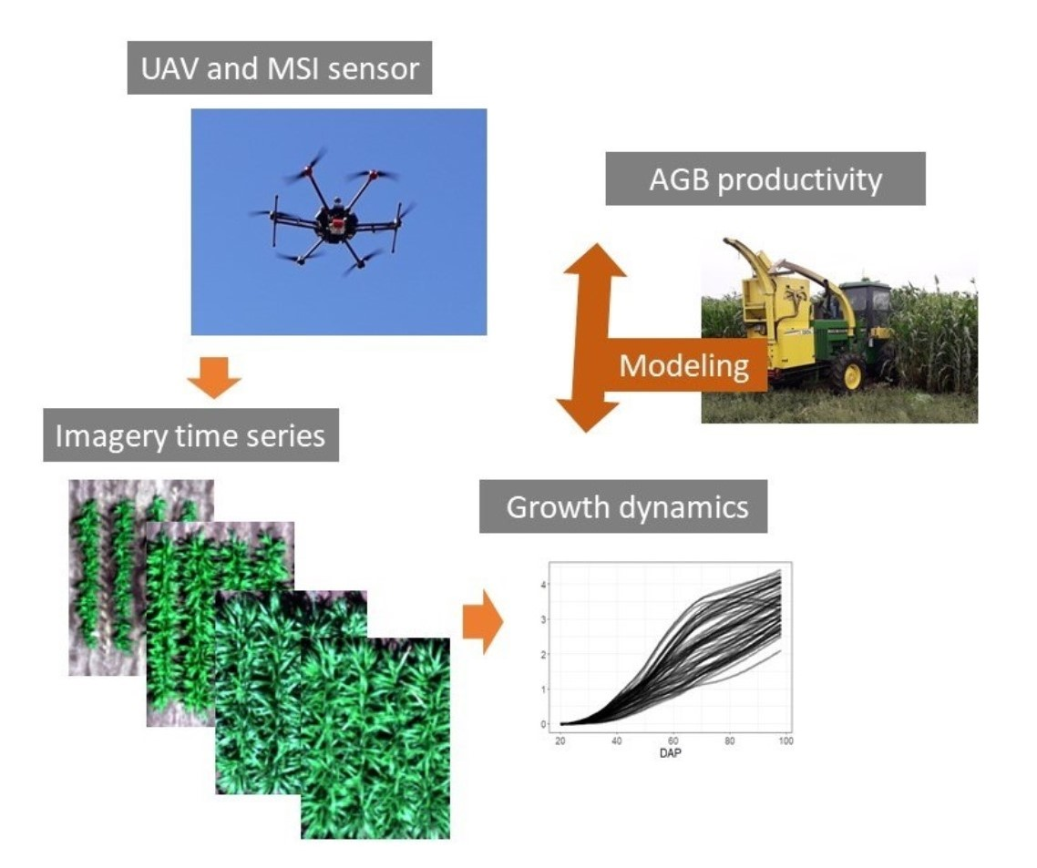
Understanding Growth Dynamics and Yield Prediction of Sorghum Using High Temporal Resolution UAV Imagery Time Series and Machine Learning

by
Sebastian Varela
1,
Taylor Pederson
2,
Carl J. Bernacchi
1,2,3,4,5 and
Andrew D. B. Leakey
1,2,4,5,6,*
1
Center for Advanced Bioenergy and Bioproducts Innovation, Urbana, IL 61801, USA
2
Institute for Genomic Biology, University of Illinois at Urbana Champaign, Urbana, IL 61801, USA
3
USDA-ARS, Global Change & Photosynthesis Research Unit, Urbana, IL 61801, USA
4
Department of Plant Biology, University of Illinois at Urbana Champaign, Urbana, IL 61801, USA
5
Center for Digital Agriculture, University of Illinois at Urbana Champaign, Urbana, IL 61801, USA
6
Department of Crop Sciences, University of Illinois at Urbana Champaign, Urbana, IL 61801, USA
*
Author to whom correspondence should be addressed.
Remote Sens. 2021, 13(9), 1763; https://doi.org/10.3390/rs13091763
Submission received: 19 February 2021 / Revised: 27 April 2021 / Accepted: 28 April 2021 / Published: 1 May 2021
(This article belongs to the Special Issue Remote and Proximal Assessment of Plant Traits)

Abstract

:
Unmanned aerial vehicles (UAV) carrying multispectral cameras are increasingly being used for high-throughput phenotyping (HTP) of above-ground traits of crops to study genetic diversity, resource use efficiency and responses to abiotic or biotic stresses. There is significant unexplored potential for repeated data collection through a field season to reveal information on the rates of growth and provide predictions of the final yield. Generating such information early in the season would create opportunities for more efficient in-depth phenotyping and germplasm selection. This study tested the use of high-resolution time-series imagery (5 or 10 sampling dates) to understand the relationships between growth dynamics, temporal resolution and end-of-season above-ground biomass (AGB) in 869 diverse accessions of highly productive (mean AGB = 23.4 Mg/Ha), photoperiod sensitive sorghum. Canopy surface height (CSM), ground cover (GC), and five common spectral indices were considered as features of the crop phenotype. Spline curve fitting was used to integrate data from single flights into continuous time courses. Random Forest was used to predict end-of-season AGB from aerial imagery, and to identify the most informative variables driving predictions. Improved prediction of end-of-season AGB (RMSE reduction of 0.24 Mg/Ha) was achieved earlier in the growing season (10 to 20 days) by leveraging early- and mid-season measurement of the rate of change of geometric and spectral features. Early in the season, dynamic traits describing the rates of change of CSM and GC predicted end-of-season AGB best. Late in the season, CSM on a given date was the most influential predictor of end-of-season AGB. The power to predict end-of-season AGB was greatest at 50 days after planting, accounting for 63% of variance across this very diverse germplasm collection with modest error (RMSE 1.8 Mg/ha). End-of-season AGB could be predicted equally well when spline fitting was performed on data collected from five flights versus 10 flights over the growing season. This demonstrates a more valuable and efficient approach to using UAVs for HTP, while also proposing strategies to add further value.

Graphical Abstract

1. Introduction

In the last 20 years, nucleic acid sequencing techniques have driven major advances in crop genomics, genetics and molecular biology [1,2]. Discovery science and crop improvement are now often limited by the speed and ease of obtaining large amounts of phenotypic information from crop trials [2,3,4]. Therefore, the development of methods for high-throughput phenotyping (HTP) of crops to reduce manual labor in the field and to better characterize phenotypes is increasingly required [3].
Recent technological advances provide new opportunities for the use of unmanned aerial vehicles (UAV) as a low-cost platform for carrying sensors that will deliver high spatial, temporal, and spectral resolution imagery to generate precise information about the interaction of solar radiation and vegetation [5]. In recent years, UAV-based structure-from-motion (SfM) techniques have been rapidly adopted to estimate traits such as canopy height [6,7] and yield [8]. Remote sensing from multispectral and hyperspectral sensors and image analysis techniques have been utilized to monitor nutrient status [9,10], above-ground biomass (AGB) [11,12], leaf area index [13,14], canopy cover [15], and senescence rate [15,16]. However, most analyses have been limited to one, or a small number, of sampling dates that are often focused towards the end of the growing season.
The tendency to focus on late-season data collection is logical given strong interest in economically important traits such as final yield or AGB. In addition, late-season phenotypes are the integrative result of all the developmental progressions and environmental conditions that occur throughout a growing season. However, there are numerous challenges associated with late-season phenotyping. Foremost, information on how the traits of interest vary across populations or treatments is often not available until very late in the season, or even after the season is complete if labor intensive destructive harvests are performed. This slows the rate of learning or discovery because material cannot be selected for more detailed analysis or breeding until the following growing season [2]. Second, damage to plants late in the growing season can introduce unwanted variation into phenotypic data. For example, while the heritability of plant height in a population of biomass sorghum increased over the first three months of the growing period, it declined in the fourth month when lodging occurred [17]. Consequently, it has been proposed that phenotyping secondary traits (e.g., green coverage, senescence rate, or crop height) that are correlated with the main target trait could avoid these problems [18].
Phenotyping as early as possible in the growing season allows more time to make decisions on subsequent sampling or selections for breeding prior to harvest for the next generation of testing [18]. Explicitly considering variation in crop phenotypes through time by repetitive monitoring can provide even greater quality data and insights about genetic and environmental variation [16,19,20,21,22,23,24]. However, collecting information repetitively over time requires a significant increase in effort and cost. So, evaluating the optimal intensity of sampling is of particular interest.
The high biomass yield potential, resource use efficiency and energy content of Sorghum bicolor (L.) Moench, along with the ability to grow on marginal lands, have made it a model C4 plant for bioenergy research worldwide [25,26,27,28]. However, sorghum performance could be further enhanced if large populations of diverse germplasm can be screened more easily using non-destructive and precise HTP methods [29]. Accurately assessing AGB is especially important and challenging for biomass crops such as photoperiod-sensitive sorghum [29]. Many genotypes achieve a final crop height of > 4 m [30]. Consequently, manual phenotyping is difficult and laborious, while mechanical harvesting requires specialized, expensive machinery [31]. With respect to HTP, the height of the crop also challenges the use of remote sensing approaches that use some ground vehicles [32,33]. In contrast, using UAVs to estimate AGB of sorghum is not hampered by the physical challenges of moving over or through the crop canopy [29]. Nevertheless, UAV-based structure from motion techniques and multispectral imagery for yield prediction have been applied to bioenergy crops much less than the major cereal crops [11,34]. Despite the rapid rate of growth achieved by these crops, most strategies have relied on single-date [29,34] or multi-date stacked imagery [5,35], meaning that information about the growth dynamics and temporal trajectory of the crop have not been exploited as a proxy of productivity. This brings opportunities to unanswered questions, e.g., what is the predictive value of repetitive screening of capturing plant growth dynamics, and how and when can we maximize information gain using UAV systems in the season?
In summary, the current work aims to investigate how SfM techniques and multispectral remote sensing data collected throughout crop development can be used to predict end-of-season AGB and to improve the efficiency and strategic use of UAVs as an HTP tool. Advances in this area are very broadly applicable because crop biomass is a core trait in many research and crop improvement programs. This includes the investigation of productivity, resource use efficiency, microbiota interactions and resilience to abiotic and biotic stresses. In the present study, the application is a characterization of genetic diversity in biomass production of sorghum as a biofuel feedstock. The nature of that variation and the high productivity of sorghum makes it a compelling test subject. Approaches to advancing the accuracy and efficiency of UAV-based phenotyping involved testing (1) the relative value of trait data from single dates versus traits describing dynamic growth as predictors of final AGB, (2) the influence of the temporal resolution of data collection (i.e., number of flights) on the prediction of final AGB, (3) how early in the season the prediction of final biomass could be achieved without a loss of accuracy, and (4) the relative value of geometric versus spectral trait data at different stages of crop development.

2. Materials and Methods

The overall workflow (Figure 1) involved: a) data collection on multiple dates from a large field trial of diverse biomass sorghum using a UAV carrying a multispectral (MSI) sensor, b) image preprocessing to produce orthophotos, (c) estimation of geometric and spectral features for each subplot on each sampling date, (d) spline curve fitting for each subplot, (e) extraction of geometric and spectral features from spline fits to produce time-point and dynamic growth variables for each subplot, (f) model training and cross-validation, (g) variable importance determination, and (h) model validation.

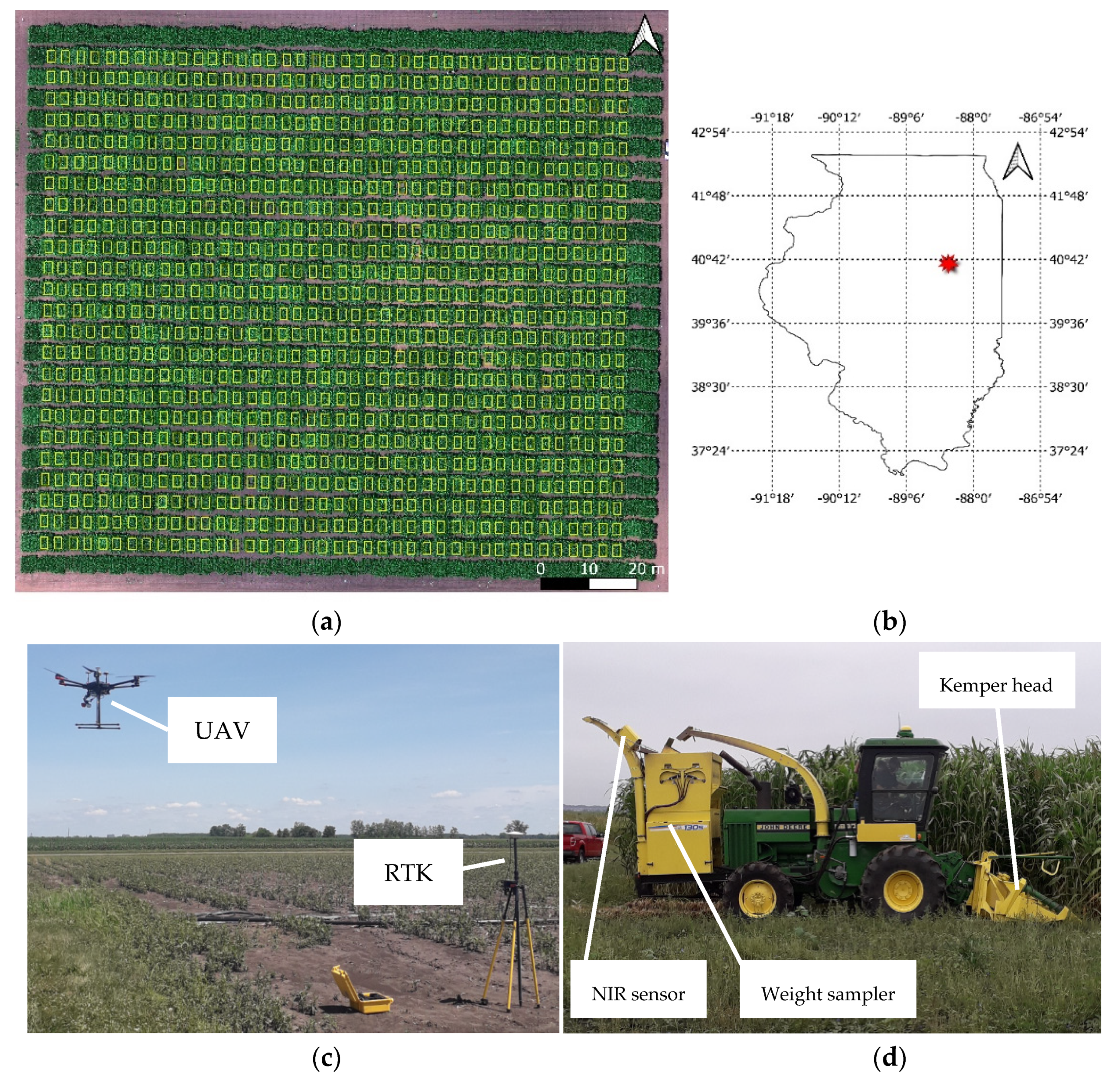
2.1. Experimental Design and Biomass Harvesting

The experiment used an augmented incomplete block design to grow 864 diverse accessions of biomass sorghum in single, four-row plots, plus six additional accessions in 16 four-row plots distributed across each of the 16 blocks, as has been previously described in detail [36,37]. The experiment was planted on May 31, 2019 at a site located at the University of Illinois Energy Farm research facility, Urbana-Champaign (40.065789°N, −88.208477°W; Figure 2a,b). Plots were harvested for AGB between September 14 and 17 using a four-row Kemper head attached to a John Deere 5830 tractor (Figure 2d). The total AGB and moisture content was determined using a plot sampler that had a near-infrared sensor (model 130S, RCI engineering). Plants in each plot were cut with the Kemper head and the harvested material entered the upper hopper of the sampler to be weighed. The material was then fed into a blower system and delivered through a spout where the near-infrared sensor is located to determine the moisture content based on established calibrations (Figure 2d). AGB in dry tons per hectare was calculated as follows: AGB dry tons/ha = total plot wet weight (kg) × (1-plot moisture) / (plot area in square meters/10,000). Strong late-season winds produced lodging damage at some specific locations in the field, making mechanical harvesting difficult. For this reason, data from the 782 undamaged plots were used for the analysis.

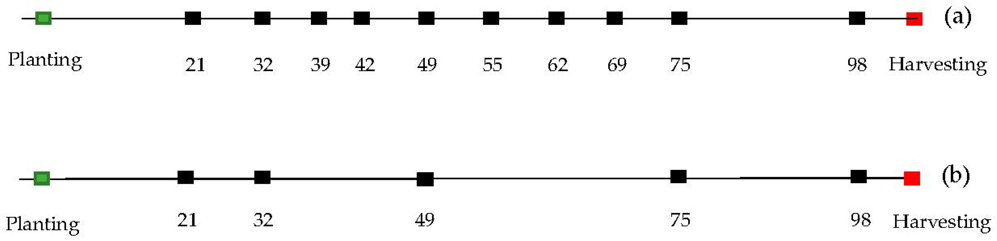
2.2. UAV System, Data Collection, and Pre-Processing

A multispectral camera (Rededge-M, Micasense, Seattle, WA, USA) was used for imaging to acquire both photogrammetric and multispectral traits. The camera is a global shutter sensor with five spectral bands in the blue (465 to 485 nm), green (550 to 570 nm), red (663 to 673 nm), rededge (712 to 722 nm), and near-infrared (820 to 860 nm) regions of the electromagnetic spectrum. The fast shutter speed of the sensor reduced blur and artifact effects in the images, which resulted in high-quality 3D reconstruction of the canopy through the season. Intrinsic optical parameters and spectral calibration correction was implemented in Metashape software (Agisoft, St. Petersburg, Russia, 2016). A standard Micasense calibration panel was imaged on the ground before and after each flight for spectral calibration. Known albedo values of the panel for each spectral band were utilized in an empirical calibration procedure as follows:
Rsunlit(i) = (Ssunlit (i) / Sref (i)) ∗ Rref(i)
In Equation (1), Ssunlit and Sref are radiance values from sunlit leaves and the reference Micasense panel, respectively, Rref refers to the reflectance of the calibration panel (calibrated, known value) provided by Micasense, and Rsunlit is the absolute reflectance of sunlit leaves in band i.
The aerial platform utilized was a Matrice 600 Pro hexacopter (DJI, Shenzhen, China), equipped with a Gremsy T1 gimbal (Gremsy, Ho Chi Minh, Vietnam) used to mount the multispectral sensor (MSI), shown in Figure 2c. Flights were conducted 10 times in the season between 21 and 98 days after planting (DAP; Figure 3a) under clear sky conditions, and between 11:00 and 13:00 local time. Flight planning allowed for 90% forward and 80% side overlapping in image acquisition following the Metashape software (Agisoft, St. Petersburg, Russia, 2016) recommendations for successful 3D reconstruction, flying at an altitude of 40 m above ground level, resulting in a ground sampling distance (GSD) of 2.5 cm/pixel. A Trimble R8 global navigation satellite system (GNSS) integrated with CORS-ILUC station was utilized for RTK (real-time kinematic) surveying of nine ground control points (GCPs) placed along the edges and the center of the experiment, with a distance of 60 to 65 m between each other. All this information was utilized for precise geo-referencing and co-registration of orthophotos between dates of data collection.
The excessive greenness index (EXG) [38] was utilized to binarize vegetation and background pixels to prevent contamination and misrepresentation of vegetation in the images. This step is necessary to mask out pixels with abnormal spectral values and regions of the image including shaded leaves and background. Pixels classified as background were masked out and not considered for the extraction of summary statistics from each plot. Green coverage (GC) is defined as the ratio of green versus total pixels in each plot. The earliest flight of the season on the day after planting (DAP) 21 was utilized as the ground level reference or digital terrain model (DTM) for the calculation of the absolute canopy height or crop surface model (CSM) on subsequent sampling dates. The results were consistent between early-season DTM and CSMs through the season. Plot polygon boundaries were delineated in QGIS v3.14.1-Pi (QGIS Geographic Information System; Open-Source Geospatial Foundation Project). Zonal statistics for each feature (Table 1) were calculated at each plot, with the 90% trimmed mean value of each feature being utilized in further analytical steps. The resulting estimates of canopy height from UAV-based images were validated against manual measurements at DAP 72 and showed a high degree of correspondence (R2 = 0.84) (Figure S1).

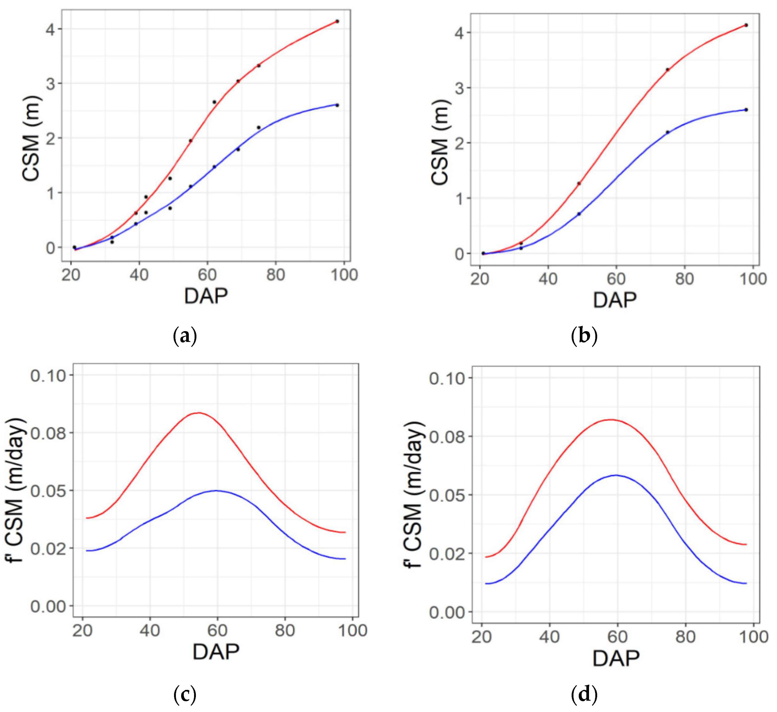
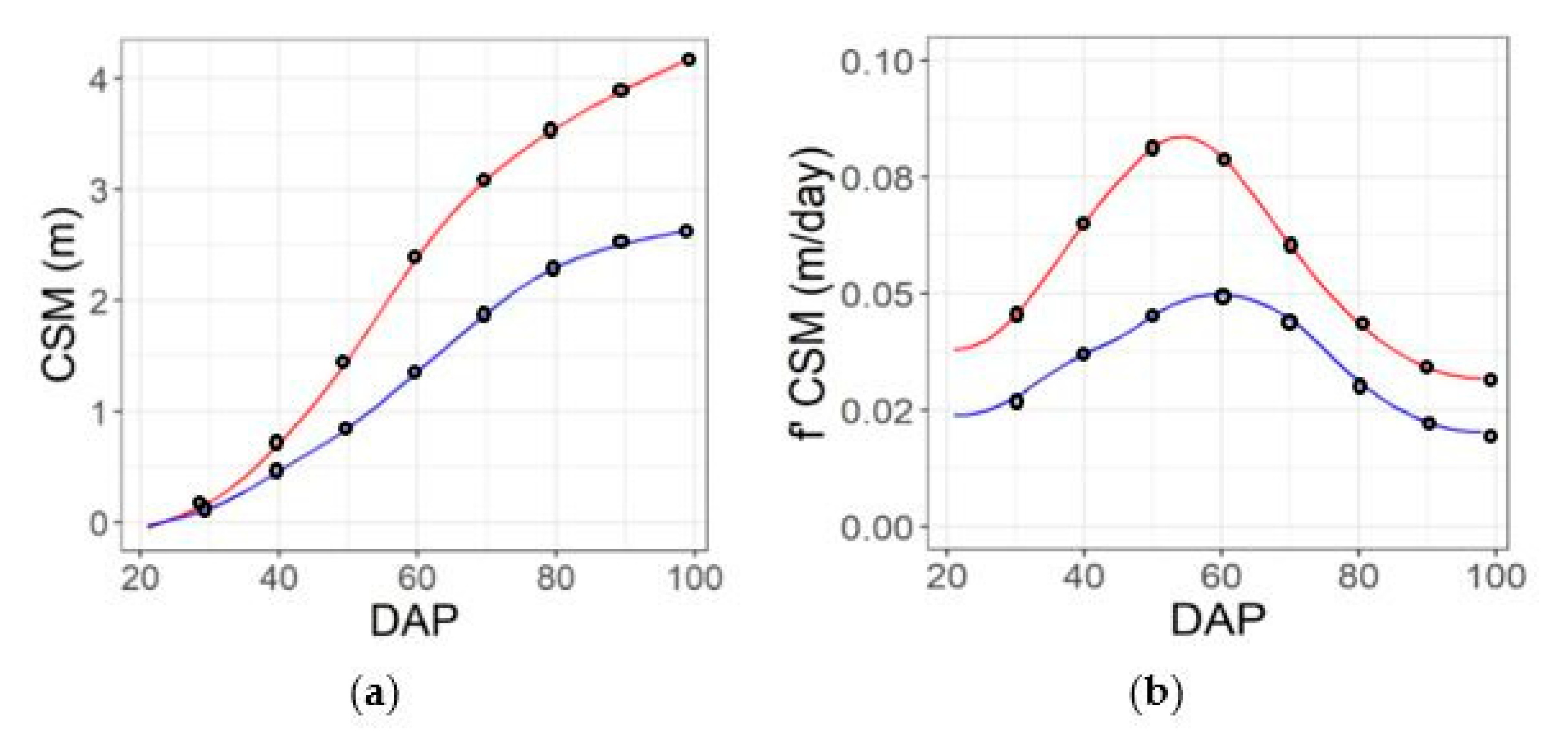
2.3. Temporal Integration via Spline Fitting

Spline fitting enabled the integration across time of information from multiple single flights, while also correcting and harmonizing for the uneven timing between flights that was caused by inclement weather conditions (e.g., precipitation or cloud cover). Consequently, an evaluation of data from individual time-point versus dynamic features of crop growth throughout the entire growing season was made possible.
Due to its particular photoperiod sensitivity [43], biomass sorghum continues to produce new vegetative biomass throughout the growing season at this location. Therefore, the growth trajectory of the crop does not clearly plateau as annual crops with a strong mid-season vegetative-reproductive transition do. This continued vegetative growth makes the traditional approach of fitting Gompertz or logistic curves to data challenging for this crop. Cubic smoothing splines have been successfully utilized [44] to characterize the growth of plants over time. It is a flexible curve-fitting technique that integrates cubic splines and curvature minimization to create an effective data modeling tool that preserves the relevant signal but removes uninformative noise in the temporal profile [45]. Specifically, a penalized criterion known as the penalized sum of squares (PSS) is defined for cubic smoothing splines (Equation (2)). The combination of both functional constraints makes smoothing splines a suitable and flexible alternative to characterize the growth dynamics of biomass sorghum.
PSS = i = 1 n ( y i S ( x i ) ) 2 + λ   S ( x ) ) 2 d x
In Equation (2), the penalized sum squares criterion is defined, the integration occurs over the range of x and λ is a tuning parameter. The first portion of the equation defines a first functional constraint that minimizes the squared error between the data and spline; the second portion of the equation considers a second constraint that directly penalizes the curve flexibility.
The smooth.spline function of the stats library in R software (R Core Team, Vienna, Austria, 2019) was utilized to implement spline fitting for each plot. The function used the input data as knots and used generalized cross-validation (GCV) to prevent under- or overfitting of the spline lambda parameter [46,47] and find an optimal level of smoothing. The minimum number of knots used was four, which is coincident with the minimum number of flights considered for the spectral features in flight pattern b (Figure S3b). The function was set to return an approximation of a continuous solution on a daily time-step over the interval of the flights (e.g., Figure 4a,b, Figures S2a,b and S3a,b) as well as the first derivative of that solution (e.g., Figure 4c,d, Figures S2c,d and S3c,d) (Table 1). Finally, the solution and its first derivative were returned at eight specific predefined dates, as described in Figure 5. In order to test the effect of the sampling frequency, the spline fitting procedure described above was applied to data from five dates (Figure 3b), as well as the full set of 10 dates (Figure 3a).
After spline fitting, the value of each of the seven features (Table 1) and the first derivative for each trait was extracted at eight predefined DAPs (30, 40, 50, 60, 70, 80, 90, 98) for each subplot (e.g., Figure 5). With eight dates and seven features (Table 1) assessed as both single time-point and dynamic traits, 112 traits were generated in total. Traits were named using the convention of “type of feature_DAP_type of variable”. For example, “NDRE_40_tp” describes NDRE on DAP 40 as a single time-point trait, while “DSM_30_slp” describes the first derivative of canopy height at DAP 30 as a dynamic growth trait.

2.4. Machine Learning Algorithm and Variable Importance

Random Forest (RF) was selected over other machine learning methods because, as a non-parametric tool, it (1) does not assume the data is normally distributed and (2) does not make assumptions about the form of associations between predictor variables and the response variable, while (3) simultaneously using multiple predictors [48]. Furthermore, as an ensemble of trees, RF is more capable in terms of prediction power and reduces overfitting compared to simple tree learners [49]. RF was used for two purposes: (i) to assess the relevance of features on prediction, and (ii) as a tool to predict AGB.
Conditional inference trees were used to build the ensembles (forests) using the cforest function [50] via caret library [51] in R software. The use of permutation importance via cforest function ensures feature selection was not biased towards predictors with many possible splits [48]. This variable importance procedure [49] has been demonstrated to reduce bias compared with other alternatives [52]. Furthermore, since the dataset includes correlated features (Figures S4 and S5), variable importance was evaluated using a conditional permutation test to minimize the overestimation on importance scores of correlated features [48].

2.5. Prediction Models

Three model configurations were tested for the prediction of end-of-season AGB {y} from a series of input variables {x1, x2, …xn} at each predefined DAP, with the aim of quantifying the relative contribution and AGB predictability of time-point and dynamic features throughout the season:
Model 1:
(time-point feature x1+…+ xk) = {AGB}
Model 2:
(dynamic feature x1 +…+ xn) = {AGB}
Model 3:
(time-point feature x1 +…+ xk + dynamic feature x1 +…+ xn) = {AGB}
Data from the 782 subplots were randomly assigned for either training (70%) or testing (30%) the model. A tenfold repeated cross-validation resampling procedure was utilized for model training. During the training process, parameters mtry (number of variables at each tree node) and ntree (number of trees) were optimized using a grid search approach, which found the optimal parameter combination by minimizing the root mean square error (RMSE). The out-of-bag sample was not used to generate the actual tree, but was used to determine the permutation importance score of each variable by accounting for the increase in mean square error of the prediction once a variable was removed from the model [49]. Each model fitting was iterated 10 times using a random training and testing partition as a measure of uncertainty of the model at each predefined DAP. At each iteration, the best-tuned model was exposed to the unknown test dataset to evaluate how the trained model generalized the prediction of AGB.
The root mean square error (RMSE), mean absolute error (MAE), absolute error (AE), and coefficient of determination (R2) were utilized as evaluation metrics to determine the performance of the models. Each metric is described in Equations (3)–(6):
RMSE = 1 n   i = 1 n   ( y i y ^ i ) 2
MAE = 1 n   i = 1 n | y i y ^ i |
AE = 100 * i = 1 n | ( y i y ^ i ) / y i | n
R 2 = 1 [ i = 1 n   ( y i y ^ i )   2 /   i = 1 n   ( y i y i ¯ 2 ) ]
In Equations (3)–(6), y , y ^ , and y ¯ are the observed, predicted, and observed mean AGB values of the ith plot, and n is the total number of samples within the study area.

3. Results

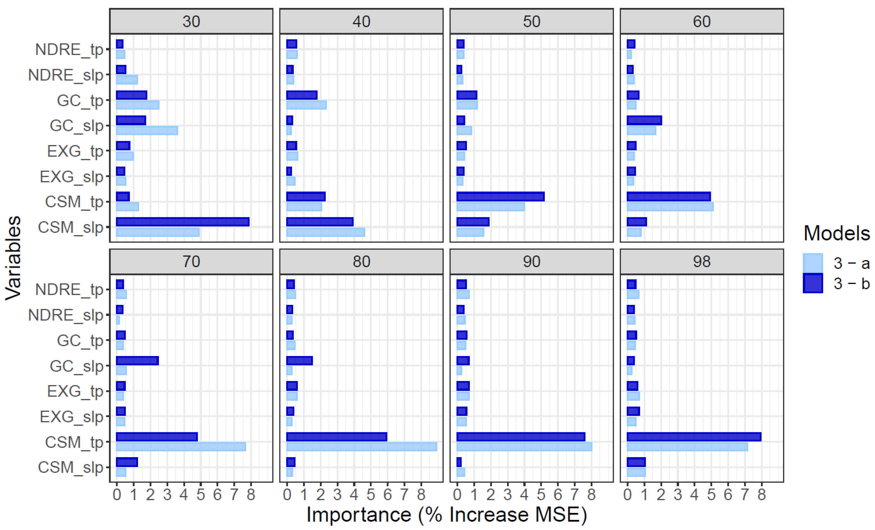
3.1. Variable Importance
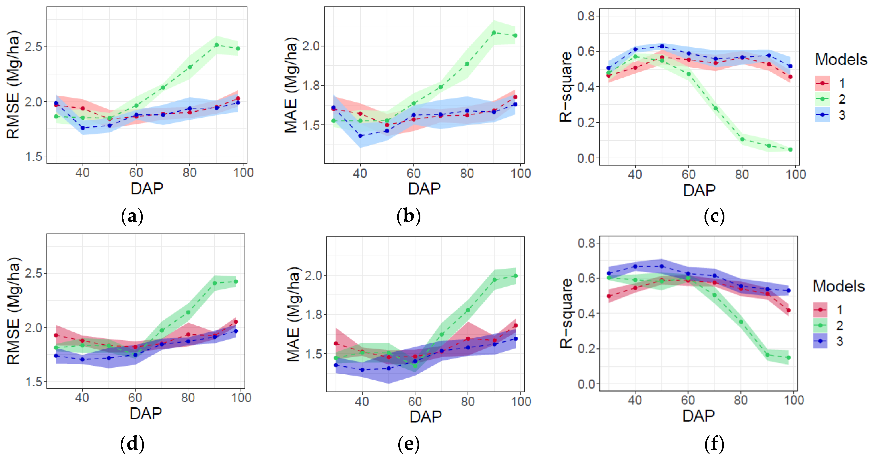
Analysis of variable importance focused on model 3 where all variables were available to inform predictions of end-of-season AGB. The relative importance of different variables to predictions of end-of-season AGB by model 3 were very similar for datasets produced from 10 flights or five flights distributed across the growing season (Figure 6). Geometric features describing the height (CSM) and ground cover (GC) of the crop canopy were generally more influential in predictions of end-of-season AGB by model 3 than spectral features such as EXG, NDRE or NDVI. This was the case regardless of which timepoint of data predictions were based on, and for both single time-point (*_tp) traits or the rate of change of the trait value on a given date (*_slp). However, the importance of individual features varied over the growing season (Figure 6). In general, GC was more important prior to canopy closure, which occurred around 60 DAP (Figure S2); dynamic variables describing the rate of change of traits were more important early in the season rather than late in the season (Figure 6).
Specifically, on the earliest date (30 DAP) the rate of height growth (CSM_slp), the rate of gain of ground cover (GC_slp), and the absolute GC on that date (GC_tp) were the most important variables for prediction of AGB by model 3. Over the subsequent month, the canopy height on given date (CSM_tp) became progressively more important. Meanwhile, CSM_slp and, to a lesser degree, GC_tp and GC_slp became progressively less important. Late in the season, from 70 to 98 DAP, CSM_tp was the only very important variable. The spectral features of NDRE_slp, NDRE_tp, EXG_slp and EXG_tp were of only moderate importance throughout the growing season, but did explain residual variance after geometric features were accounted for (Figure 6).

3.2. AGB Prediction

Using data from five rather than 10 flights did not significantly reduce the performance of any of the three categories of models or alter their relative performance in terms of RMSE, MAE, and R2 (Figure 7). Moreover, predictions based on data from both flight patterns evidenced a similar prediction stability, as indicated by their standard deviations (Figure 7d–f) and for predictions based on data from 10 flights (Figure 7a–c).
Combining single-time-point and dynamic variables in model 3 generally resulted in the best and most consistent performance in terms of RMSE, MAE and R2 throughout the growing season (Figure 7). Error was lowest (RMSE = 1.7–1.8 Mg/ha; MAE = 1.3–1.5 Mg/ha) and the proportion of variance explained was greatest (R2 = 0.59–0.63) for model 3 between DAPs 40 and 50, i.e., shortly prior to canopy closure. Model 1 performed essentially equivalently to model 3 when based on single-time-point data collected after canopy closure (>70 DAP). However, predictions of end-of-season AGB by model 1 were less accurate and explained less variance than model 3 when based on early-season data. In contrast, predictions by model 2 were better when based on dynamic variables measured early versus late in the growing season. However, even model 2 did not perform as well as model 3 prior to canopy closure.

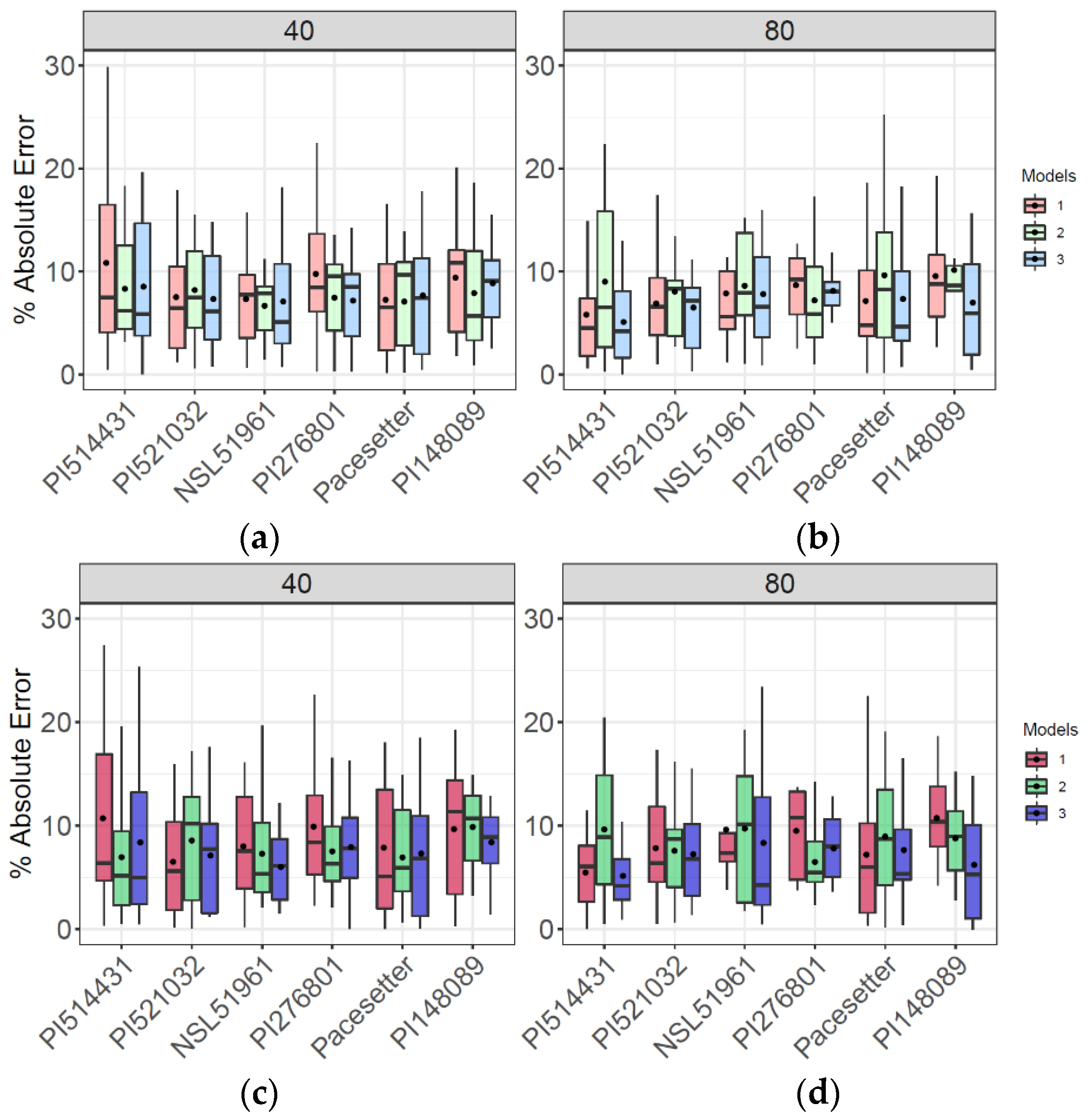
3.3. AGB Prediction for Six Accessions Tested in Highly Replicated (n = 16) Plots

Mean end-of-season AGB varied from 21 to 27.6 Mg/ha across six accessions grown in highly replicated (n = 16) plots (Figure S9). However, equivalent or greater variation in AGB was observed among the 16 replicate plots of each accession (Figure S9). Consistent with results for the population as a whole (Figure 7), combining single time-point variables and dynamic variables in model 3 produced accurate and consistent results at both the early season stage (DAP 40) and after canopy closure (DAP 80) (Figure 8). By contrast, and more clearly marked in the reduced number of flights pattern, single time-point variables model 1 produced higher mean AE early in the season (Figure 8a,c) in three and four of the six genotypes of each flight patterns, respectively. Aligned with the whole population prediction, using only dynamic variables in model 2 produced higher AE late in the season (Figure 8), where the predicted AGB does not align accordingly with the observed values (Figure S9b,d).
Even with model 3, there is a tendency towards underestimating the end-of-season AGB of the most productive genotypes (e.g., PI148089; Figure S9b,d). However, that was less the case early in the season (DAP 40) than late in the season (DAP 80). A general pattern of bias leading to underestimations of AGB in high-yielding genotypes was evident in the population as a whole (Figure S8). The variance among replicate plots of a given genotype was often substantially less for model predictions of end-of-season AGB than it was for data from the mechanical harvest (Figure S9). Again, a reduction in the number of flights from 10 to five did not substantially affect how models 1, 2, or 3 performed in predicting AGB of these highly replicated accessions, as seen in Figure S9.

3.4. Trait Relationships

Patterns of pairwise correlations among traits were very similar for datasets based on spline fitting of data from 10 flights per season (Figure S4) compared to five flights per season (Figure S5). So, interpretation of the results will focus on the use of the full dataset from 10 flights. Trait relationships varied significantly over the course of the growing season (Figure S4). Early in the season (DAP 30, 40, 50, 60), many measures of growth rate and absolute size were associated with each other; i.e., there were positive correlations among the single time-point spectral traits (NDVI_tp, NDRE_tp, WDRVI_tp, NGRDI_tp), the single time-point geometric traits (CSM_tp, GC_tp), the rate of canopy growth both vertically (CSM_slp) and horizontally (GC_slp), as well as end-of-season AGB (Figure S4). In contrast, on DAP 30 and DAP 40, the initial rates of gain of spectral indices were correlated with each other, but not with the single-time-point spectral or geometric traits describing absolute plant sizes. Additionally, during the period when canopy closure occurred for different genotypes (DAP 50, 60, 70), the rates of gain of ground cover (GC_slp) and spectral traits (NDVI_slp, NDRE_ slp, WDRVI_ slp, NGRDI_ slp, EXG_slp) became negatively correlated with single time-point measures of geometric and spectral variables (CSM_tp, GC_tp, NDVI_tp, NDRE_tp, WDRVI_tp, NGRDI_tp; Figure S4). Late in the growing season, there were no significant correlations among the single time-point traits and dynamic traits describing the rate of change of either geometric or spectral features. However, there was still a significant correlation between canopy height and end-of-season AGB.

4. Discussion

This study successfully addressed its goals by demonstrating that early- and mid-season measurement of dynamic growth traits by UAV can be combined with individual time-point trait data to facilitate improved prediction of end-of-season AGB (Figure 6 and Figure 7). Specifically, data on the rate of change of geometric and spectral features extracted from multispectral imagery of biomass sorghum canopies resulted in more accurate predictions of end-of-season AGB at much earlier dates in the growing season. In addition, end-of-season AGB could be predicted equally well when spline fitting was performed on data collected from five flights versus 10 flights over the growing season. The resulting analysis revealed limitations and opportunities for HTP of genetic variation in the productivity of photoperiod sensitive biomass sorghum accessions, which presents special challenges as a result of its delayed transition to reproductive development and high AGB.
Geometric and spectral information have proved to be relevant descriptors of biomass in annual grain crops such as rice [53], barley [54,55], and wheat [56]. Spectral information has proved to be an important proxy for AGB prediction in annual grain crops in these studies, but prediction accuracy significantly increased when integrating both types of traits in the same model [54,56]. It was also pointed out that geometric features provided more robust AGB prediction results in barley [55] and wheat [56] or provided both similar prediction power in rice [53]. In our study, geometric information is consistently the more influential descriptor of final biomass than spectral information, regardless of whether it is being considered as a trait reported at a single time-point or as a dynamic trait describing a rate of change over time (Figure 6). This is consistent with canopy height previously being identified as a trait that displays significant intraspecific variation, with high heritability, in other species [53,54,55,56,57,58]. This is probably, in part, because it does not suffer from signal saturation as spectral information does late in the growing season. Biomass sorghum shows a rapid increase in ground cover and vertical growth, such that canopy closure and heights of ~1.5 to 2.5 m are achieved at around 50 to 70 DAP (Figure 4 and Figure S2). The power to predict end-of-season AGB was greatest around DAP 50, presumably because this gave the genetic variation present in the large diverse population of accessions the greatest period of time to express itself in AGB before occlusion associated with canopy closure made it harder to image the size and structure of vegetative structures. Demonstrating the value of measuring early-season dynamic variables is a departure from the conclusions of previous studies where only single time-point data were analyzed and the best predictions of biomass were found using mid- and late-season data [18,32]. However, there is still the common finding that single time-point height data is a key predictor of end-of-season AGB when measured late in the growing season. Moreover, it is important to recognize that stressful or extreme weather conditions late in the season could cause end-of-season AGB to deviate from what is predicted from early-season indicators of productivity. So, additional analyses across multiple years or locations will be needed to establish how robust the findings of this study are across environmental variation.
Highly replicated plots (n = 16) of six genotypes provided a valuable test of HTP methods that complemented the broader survey of the full population of biomass sorghum. The results were very similar to what is described above in terms of the value of geometric versus spectral traits early versus late in the growing season and with data from 10 flights versus five flights. It was notable that the underestimation of end-of-season AGB in the highest productivity line by model 3 (time-point + dynamic variables) was less in early-season predictions based on dynamic traits than in late-season predictions driven mainly by single time-point height data (Figure 8). It could be argued that the general underestimation of AGB in high-productivity accessions is directly related to the distribution of the AGB data with regard to extreme values [5]. There was substantial variability in end-of-season AGB across the 16 replicate plots of these six accessions. Some of this will have resulted from spatial variability across the field, but there is also likely significant variation associated with inconsistency in biomass estimates from the forage harvester. Variability in predictions of AGB from the UAV data were notably less variable across replicate plots. Additional experiments will be needed to demonstrate whether this is a consequence of the RF modeling approach or results from UAV measurements leading to more reproducible AGB estimates than destructive harvest.
The potential to roughly predict variation in end-of-season AGB from dynamic traits at mid-season or earlier could be very valuable for a number of reasons. A subset of genotypes with desirable characteristics could be selected for: (1) seed production by crossing or selfing well in advance of key reproductive events; or (2) additional phenotyping by manual methods or other HTP techniques. In the case of short-day photoperiod sensitive sorghum, plants might even be transplanted out of the field into controlled environment conditions, where flowering could be induced earlier than would occur naturally in a mid-latitude location such as the U.S. Midwest [59]. In both cases, labor and expense could be saved within the field season and some activities could be performed without the usual need to wait for an additional generation of plants to be grown. The value of accelerating breeding cycles is well recognized in many major food crops [60], and the improvement of bioenergy crops would also benefit from this strategy.
Many previous studies indicate that spectral vegetation indices lose sensitivity when biomass accumulation is high and canopies are dense [41,42]. This is consistent with the negative correlations that were observed between the first derivative of spectral features and measures of absolute canopy size at mid-season (Figure S4). The limited value of spectral features to predictions of end-of-season AGB in the current study probably also resulted from limiting the trial to the study of genetic variation in a single environment. This is a key context in which HTP needs to be tested, but where there is not as much phenotypic variation to exploit as in experiments where environmental or management treatments such as variable nitrogen fertilization [29] or drought stress [61] are also imposed. An important practical consequence of being able to predict end-of-season AGB from dynamic geometric features early in the season is that it indicates that low-cost RGB cameras can be utilized as lower-cost alternatives to multispectral sensors without significant compromises on the value of the data collected [62].
Reducing the number of data collection flights, from 10 to five dates spaced across the growing season, did not penalize the sensitivity and ranking of variables’ importance through the season. Since the crop reaches full green coverage in a very short period (Figure S2) flights earlier than DAP 50 become critical to differentiate final productivity between genotypes. This highlights that a reduction of the number of flights can be implemented, but timing of the flights is key for specific variables. To overcome this challenge, prior understanding of the seasonal predictability of the trait of interest, as reported in this work, becomes critical for efficient use of the UAV in the season. By accounting for that, researchers will be able to prioritize collection of aerial data at stages of the crop with high information value, rather than collecting aerial data with marginal informative value, or by reconstructing the entire temporal season profile of the crop, as presented in this work.
While the method presented here provides valuable predictions of end-of-season AGB from early-season phenotype data, there is still significant unexplained variation in AGB. Sorghum accessions vary significantly in the number and diameter of stems [63,64]. Variation in those traits will be hard to detect in geometric or spectral features of aerial imagery after canopy closure. Therefore, it seems likely that aerial and ground-based imaging using rovers or push-cart mounted sensors [65,66,67] will need to be paired together to capture more of the traits needed to explain the full diversity of AGB in biomass sorghum.

5. Conclusions

This study demonstrated the use of high temporal resolution UAV imagery to understand the relative importance of dynamic and single-date static information throughout the season to predictions of final harvestable AGB. Geometric features were consistently the most informative variables of end-of-season AGB in the season. In particular, rapid rates of growth early in the season were positively associated with final productivity. In addition, by being able to identify stages of the crop with higher information gain, a more precise and efficient strategic use of the UAV as HTP tool in the season can be implemented. Spectral information was not a main descriptor of end-of-season AGB, which shows RGB sensors are expected to reach similar performance as multispectral sensors but at a lower budget. The number of visits to the field, which are an important component of the cost of operations of these platforms, can be significantly reduced with no information lost if data collection is timed appropriately. Future directions should explore the impact of the spatial resolution of imagery, and the complementary integration of the capabilities of UAV to cover large areas and high sensitivity of ground vehicles to characterize canopy architectural traits to overcome limitations associated with the occlusion of stems and the saturation of spectral features after canopy closure.

Supplementary Materials

The following are available online at https://www.mdpi.com/article/10.3390/rs13091763/s1, Figures S1–S9.

Author Contributions

S.V. and A.D.B.L. conceived the study, interpreted the data, and wrote the manuscript with input from all other authors. S.V. collected, processed and analyzed data. T.P. and C.J.B. established, maintained and harvested the field trial. All authors have read and agreed to the published version of the manuscript.

Funding

This work was funded by the DOE Center for Advanced Bioenergy and Bioproducts Innovation (U.S. Department of Energy, Office of Science, Office of Biological and Environmental Research under Award Number DE-SC0018420). Any opinions, findings, and conclusions or recommendations expressed in this publication are those of the author(s) and do not necessarily reflect the views of the U.S. Department of Energy.

Data Availability Statement

The datasets used and analyzed during the current study are available from the corresponding author via Illinois Databank at https://doi.org/10.13012/B2IDB-5649852_V2.

Acknowledgments

We thank Jeremy Ruther, Timothy Mies and Trace Elliot for technical assistance.

Conflicts of Interest

The authors declare no conflict of interest.

References

  1. Furbank, R.T.; Tester, M. Phenomics—Technologies to relieve the phenotyping bottleneck. Trends Plant Sci. 2011, 16, 635–644. [Google Scholar] [CrossRef]
  2. Araus, J.L.; Kefauver, S.C.; Zaman-Allah, M.; Olsen, M.S.; Cairns, J.E. Translating High-Throughput Phenotyping into Genetic Gain. Trends Plant Sci. 2018, 23, 451–466. [Google Scholar] [CrossRef] [Green Version]
  3. Zhao, C.; Zhang, Y.; Du, J.; Guo, X.; Wen, W.; Gu, S.; Wang, J.; Fan, J. Crop Phenomics: Current Status and Perspectives. Front. Plant Sci. 2019, 10, 714. [Google Scholar] [CrossRef] [PubMed] [Green Version]
  4. Pieruschka, R.; Schurr, U. Plant Phenotyping: Past, Present, and Future. Available online: https://spj.sciencemag.org/journals/plantphenomics/2019/7507131/ (accessed on 1 October 2020).
  5. Herrero-Huerta, M.; Rodriguez-Gonzalvez, P.; Rainey, K.M. Yield prediction by machine learning from UAS-based multi-sensor data fusion in soybean. Plant Methods 2020, 16, 1–16. [Google Scholar] [CrossRef] [PubMed]
  6. Malambo, L.; Popescu, S.; Murray, S.; Putman, E.; Pugh, N.; Horne, D.; Richardson, G.; Sheridan, R.; Rooney, W.; Avant, R.; et al. Multitemporal field-based plant height estimation using 3D point clouds generated from small unmanned aerial systems high-resolution imagery. Int. J. Appl. Earth Obs. Geoinf. 2018, 64, 31–42. [Google Scholar] [CrossRef]
  7. Watanabe, K.; Guo, W.; Arai, K.; Takanashi, H.; Kajiya-Kanegae, H.; Kobayashi, M.; Yano, K.; Tokunaga, T.; Fujiwara, T.; Tsutsumi, N.; et al. High-Throughput Phenotyping of Sorghum Plant Height Using an Unmanned Aerial Vehicle and Its Application to Genomic Prediction Modeling. Front. Plant Sci. 2017, 8, 421. [Google Scholar] [CrossRef] [PubMed] [Green Version]
  8. Roth, L.; Streit, B. Predicting cover crop biomass by lightweight UAS-based RGB and NIR photography: An applied photogrammetric approach. Precis. Agric. 2017, 19, 93–114. [Google Scholar] [CrossRef] [Green Version]
  9. Zheng, H.; Li, W.; Jiang, J.; Liu, Y.; Cheng, T.; Tian, Y.; Zhu, Y.; Cao, W.; Zhang, Y.; Yao, X. A Comparative Assessment of Different Modeling Algorithms for Estimating Leaf Nitrogen Content in Winter Wheat Using Multispectral Images from an Unmanned Aerial Vehicle. Remote Sens. 2018, 10, 2026. [Google Scholar] [CrossRef] [Green Version]
  10. Wang, H.; Mortensen, A.K.; Mao, P.; Boelt, B.; Gislum, R. Estimating the nitrogen nutrition index in grass seed crops using a UAV-mounted multispectral camera. Int. J. Remote Sens. 2019, 40, 2467–2482. [Google Scholar] [CrossRef]
  11. Masjedi, A.; Zhao, J.; Thompson, A.M.; Yang, K.-W.; Flatt, J.E.; Crawford, M.M.; Ebert, D.S.; Tuinstra, M.R.; Hammer, G.; Chapman, S. Sorghum Biomass Prediction Using Uav-Based Remote Sensing Data and Crop Model Simulation. In Proceedings of the IGARSS 2018—2018 IEEE International Geoscience and Remote Sensing Symposium, Valencia, Spain, 22–27 July 2018; pp. 7719–7722. [Google Scholar]
  12. Grüner, E.; Wachendorf, M.; Astor, T. The potential of UAV-borne spectral and textural information for predicting aboveground biomass and N fixation in legume-grass mixtures. PLoS ONE 2020, 15, e0234703. [Google Scholar] [CrossRef]
  13. Verrelst, J.; Rivera, J.P.; Veroustraete, F.; Muñoz-Marí, J.; Clevers, J.G.; Camps-Valls, G.; Moreno, J. Experimental Sentinel-2 LAI estimation using parametric, non-parametric and physical retrieval methods—A comparison. ISPRS J. Photogramm. Remote Sens. 2015, 108, 260–272. [Google Scholar] [CrossRef]
  14. Potgieter, A.B.; George-Jaeggli, B.; Chapman, S.C.; Laws, K.; Cadavid, L.A.S.; Wixted, J.; Watson, J.; Eldridge, M.; Jordan, D.R.; Hammer, G.L. Multi-Spectral Imaging from an Unmanned Aerial Vehicle Enables the Assessment of Seasonal Leaf Area Dynamics of Sorghum Breeding Lines. Front. Plant Sci. 2017, 8, 1532. [Google Scholar] [CrossRef] [PubMed]
  15. Makanza, R.; Zaman-Allah, M.; Cairns, J.E.; Magorokosho, C.; Tarekegne, A.; Olsen, M.; Prasanna, B.M. High-Throughput Phenotyping of Canopy Cover and Senescence in Maize Field Trials Using Aerial Digital Canopy Imaging. Remote Sens. 2018, 10, 330. [Google Scholar] [CrossRef] [Green Version]
  16. Hassan, M.A.; Yang, M.; Rasheed, A.; Jin, X.; Xia, X.; Xiao, Y.; He, Z. Time-Series Multispectral Indices from Unmanned Aerial Vehicle Imagery Reveal Senescence Rate in Bread Wheat. Remote Sens. 2018, 10, 809. [Google Scholar] [CrossRef] [Green Version]
  17. Fernandes, S.B.; Dias, K.O.G.; Ferreira, D.F.; Brown, P.J. Efficiency of multi-trait, indirect, and trait-assisted genomic selection for improvement of biomass sorghum. Theor. Appl. Genet. 2018, 131, 747–755. [Google Scholar] [CrossRef] [Green Version]
  18. Bustos-Korts, D.; Boer, M.P.; Malosetti, M.; Chapman, S.; Chenu, K.; Zheng, B.; van Eeuwijk, F.A. Combining Crop Growth Modeling and Statistical Genetic Modeling to Evaluate Phenotyping Strategies. Front. Plant Sci. 2019, 10. [Google Scholar] [CrossRef]
  19. van Eeuwijk, F.A.; Bustos-Korts, D.; Millet, E.J.; Boer, M.P.; Kruijer, W.; Thompson, A.; Malosetti, M.; Iwata, H.; Quiroz, R.; Kuppe, C.; et al. Modelling strategies for assessing and increasing the effectiveness of new phenotyping techniques in plant breeding. Plant Sci. 2019, 282, 23–39. [Google Scholar] [CrossRef]
  20. Pugh, N.A.; Horne, D.W.; Murray, S.C.; Carvalho, G.; Malambo, L.; Jung, J.; Chang, A.; Maeda, M.; Popescu, S.; Chu, T.; et al. Temporal Estimates of Crop Growth in Sorghum and Maize Breeding Enabled by Unmanned Aerial Systems. Plant Phenome J. 2018, 1, 1–10. [Google Scholar] [CrossRef]
  21. Malosetti, M.; Visser, R.G.F.; Celis-Gamboa, C.; van Eeuwijk, F.A. QTL methodology for response curves on the basis of non-linear mixed models, with an illustration to senescence in potato. Theor. Appl. Genet. 2006, 113, 288–300. [Google Scholar] [CrossRef]
  22. Van Eeuwijk, F.A.; Bink, M.C.A.M.; Chenu, K.; Chapman, S.C. Detection and use of QTL for complex traits in multiple environments. Curr. Opin. Plant Biol. 2010, 13, 193–205. [Google Scholar] [CrossRef]
  23. Hurtado-Lopez, P.X.; Tessema, B.B.; Schnabel, S.K.; Maliepaard, C.; van der Linden, C.G.; Eilers, P.H.C.; Jansen, J.; van Eeuwijk, F.A.; Visser, R.G.F. Understanding the genetic basis of potato development using a multi-trait QTL analysis. Euphytica 2015, 204, 229–241. [Google Scholar] [CrossRef] [Green Version]
  24. Rutkoski, J.; Poland, J.; Mondal, S.; Autrique, E.; Pérez, L.G.; Crossa, J.; Reynolds, M.; Singh, R. Canopy Temperature and Vegetation Indices from High-Throughput Phenotyping Improve Accuracy of Pedigree and Genomic Selection for Grain Yield in Wheat. G3 Genes Genomes Genet. 2016, 6, 2799–2808. [Google Scholar] [CrossRef] [Green Version]
  25. Xin, Z.; Wang, M.L. Sorghum as a versatile feedstock for bioenergy production. Biofuels 2011, 2, 577–588. [Google Scholar] [CrossRef]
  26. De Oliveira, A.A.; Pastina, M.M.; de Souza, V.F.; Parrella, R.A.D.C.; Noda, R.W.; Simeone, M.L.F.; Schaffert, R.E.; de Magalhães, J.V.; Damasceno, C.M.B.; Margarido, G.R.A. Genomic prediction applied to high-biomass sorghum for bioenergy production. Mol. Breed. 2018, 38, 1–16. [Google Scholar] [CrossRef] [Green Version]
  27. Rao, P.S.; Vinutha, K.S.; Kumar, G.S.A.; Chiranjeevi, T.; Uma, A.; Lal, P.; Prakasham, R.S.; Singh, H.P.; Rao, R.S.; Chopra, S.; et al. Sorghum: A Multipurpose Bioenergy Crop. In Agronomy Monographs; American Society of Agronomy and Crop Science: Madison, WI, USA, 2016; ISBN 9780891186281. [Google Scholar]
  28. Prakasham, R.S.; Nagaiah, D.; Vinutha, K.S.; Uma, A.; Chiranjeevi, T.; Umakanth, A.V.; Rao, P.S.; Yan, N. Sorghum biomass: A novel renewable carbon source for industrial bioproducts. Biofuels 2014, 5, 159–174. [Google Scholar] [CrossRef] [Green Version]
  29. Li, J.; Shi, Y.; Veeranampalayam-Sivakumar, A.-N.; Schachtman, D.P. Elucidating Sorghum Biomass, Nitrogen and Chlorophyll Contents with Spectral and Morphological Traits Derived from Unmanned Aircraft System. Front. Plant Sci. 2018, 9, 1406. [Google Scholar] [CrossRef] [PubMed]
  30. Hoffmann, L.L.; Rooney, W.L. Accumulation of Biomass and Compositional Change Over the Growth Season for Six Photoperiod Sorghum Lines. BioEnergy Res. 2014, 7, 811–815. [Google Scholar] [CrossRef]
  31. Habyarimana, E.; Piccard, I.; Catellani, M.; de Franceschi, P.; Dall’Agata, M. Towards Predictive Modeling of Sorghum Biomass Yields Using Fraction of Absorbed Photosynthetically Active Radiation Derived from Sentinel-2 Satellite Imagery and Supervised Machine Learning Techniques. Agronomy 2019, 9, 203. [Google Scholar] [CrossRef] [Green Version]
  32. Andrade-Sanchez, P.; Gore, M.A.; Heun, J.T.; Thorp, K.R.; Carmo-Silva, A.E.; French, A.N.; Salvucci, M.E.; White, J.W. Development and evaluation of a field-based high-throughput phenotyping platform. Funct. Plant Biol. 2014, 41, 68–79. [Google Scholar] [CrossRef] [Green Version]
  33. Jimenez-Berni, J.A.; Deery, D.M.; Rozas-Larraondo, P.; Condon, A.G.; Rebetzke, G.J.; James, R.A.; Bovill, W.D.; Furbank, R.T.; Sirault, X.R.R. High Throughput Determination of Plant Height, Ground Cover, and Above-Ground Biomass in Wheat with LiDAR. Front. Plant Sci. 2018, 9, 237. [Google Scholar] [CrossRef] [Green Version]
  34. Cholula, U.; da Silva, J.A.; Marconi, T.; Thomasson, J.A.; Solorzano, J.; Enciso, J. Forecasting Yield and Lignocellulosic Composition of Energy Cane Using Unmanned Aerial Systems. Agronomy 2020, 10, 718. [Google Scholar] [CrossRef]
  35. Li, J.; Veeranampalayam-Sivakumar, A.-N.; Bhatta, M.; Garst, N.D.; Stoll, H.; Baenziger, P.S.; Belamkar, V.; Howard, R.; Ge, Y.; Shi, Y. Principal variable selection to explain grain yield variation in winter wheat from features extracted from UAV imagery. Plant Methods 2019, 15, 1–13. [Google Scholar] [CrossRef] [PubMed]
  36. Valluru, R.; Gazave, E.E.; Fernandes, S.B.; Ferguson, J.N.; Lozano, R.; Hirannaiah, P.; Zuo, T.; Brown, P.J.; Leakey, A.D.B.; Gore, M.A.; et al. Deleterious Mutation Burden and Its Association with Complex Traits in Sorghum (Sorghum bicolor). Genetics 2019, 211, 1075–1087. [Google Scholar] [CrossRef] [PubMed] [Green Version]
  37. Dos Santos, J.P.R.; Fernandes, S.B.; McCoy, S.; Lozano, R.; Brown, P.J.; Leakey, A.D.B.; Buckler, E.S.; Garcia, A.A.F.; Gore, M.A. Novel Bayesian Networks for Genomic Prediction of Developmental Traits in Biomass Sorghum. G3 Genes Genomes Genet. 2020, 10, 769–781. [Google Scholar] [CrossRef] [PubMed] [Green Version]
  38. Woebbecke, D.M.; Meyer, G.E.; von Bargen, K.; Mortensen, D.A. Color Indices for Weed Identification Under Various Soil, Residue, and Lighting Conditions. Trans. ASAE 1995, 38, 259–269. [Google Scholar] [CrossRef]
  39. Wu, M.; Yang, C.; Song, X.; Hoffmann, W.C.; Huang, W.; Niu, Z.; Wang, C.; Li, W. Evaluation of Orthomosics and Digital Surface Models Derived from Aerial Imagery for Crop Type Mapping. Remote Sens. 2017, 9, 239. [Google Scholar] [CrossRef] [Green Version]
  40. Wahab, I.; Hall, O.; Jirström, M. Remote Sensing of Yields: Application of UAV Imagery-Derived NDVI for Estimating Maize Vigor and Yields in Complex Farming Systems in Sub-Saharan Africa. Drones 2018, 2, 28. [Google Scholar] [CrossRef] [Green Version]
  41. Gitelson, A.A. Wide Dynamic Range Vegetation Index for Remote Quantification of Biophysical Characteristics of Vegetation. J. Plant Physiol. 2004, 161, 165–173. [Google Scholar] [CrossRef] [PubMed] [Green Version]
  42. Moges, S.M.; Raun, W.; Mullen, R.W.; Freeman, K.W.; Johnson, G.V.; Solie, J.B. Evaluation of Green, Red, and Near Infrared Bands for Predicting Winter Wheat Biomass, Nitrogen Uptake, and Final Grain Yield. J. Plant Nutr. 2005, 27, 1431–1441. [Google Scholar] [CrossRef]
  43. Meki, M.N.; Ogoshi, R.M.; Kiniry, J.R.; Crow, S.E.; Youkhana, A.H.; Nakahata, M.H.; Littlejohn, K. Performance evaluation of biomass sorghum in Hawaii and Texas. Ind. Crop. Prod. 2017, 103, 257–266. [Google Scholar] [CrossRef] [Green Version]
  44. Brien, C.; Jewell, N.; Watts-Williams, S.J.; Garnett, T.; Berger, B. Smoothing and extraction of traits in the growth analysis of noninvasive phenotypic data. Plant Methods 2020, 16, 1–21. [Google Scholar] [CrossRef] [PubMed]
  45. Green, P.J.; Silverman, B.W. Nonparametric Regression and Generalized Linear Models: A Roughness Penalty Approach; Chapman and Hall: London, UK, 1994; ISBN 9780412300400. [Google Scholar]
  46. Lukas, M.A.; de Hoog, F.R.; Anderssen, R.S. Efficient algorithms for robust generalized cross-validation spline smoothing. J. Comput. Appl. Math. 2010, 235, 102–107. [Google Scholar] [CrossRef] [Green Version]
  47. Phillips, G.M.; Taylor, P.J. Splines and Other Approximations. In Theory and Applications of Numerical Analysis, 2nd ed.; Phillips, G.M., Taylor, P.J., Eds.; Academic Press: London, UK, 1996; pp. 131–159. ISBN 9780125535601. [Google Scholar]
  48. Probst, P.; Wright, M.N.; Boulesteix, A. Hyperparameters and tuning strategies for random forest. Wiley Interdiscip. Rev. Data Min. Knowl. Discov. 2019, 9, 9. [Google Scholar] [CrossRef] [Green Version]
  49. Breiman, L. Random Forests. Mach. Learn. 2001, 45, 5–32. [Google Scholar] [CrossRef] [Green Version]
  50. Hothorn, T.; Hornik, K.; Zeileis, A. Unbiased Recursive Partitioning: A Conditional Inference Framework. J. Comput. Graph. Stat. 2006, 15, 651–674. [Google Scholar] [CrossRef] [Green Version]
  51. Kuhn, M. Building Predictive Models in RUsing thecaretPackage. J. Stat. Softw. 2008, 28, 1–26. [Google Scholar] [CrossRef] [Green Version]
  52. Strobl, C.; Boulesteix, A.-L.; Zeileis, A.; Hothorn, T. Bias in random forest variable importance measures: Illustrations, sources and a solution. BMC Bioinform. 2007, 8, 25. [Google Scholar] [CrossRef] [PubMed] [Green Version]
  53. Jiang, Q.; Fang, S.; Peng, Y.; Gong, Y.; Zhu, R.; Wu, X.; Ma, Y.; Duan, B.; Liu, J. UAV-Based Biomass Estimation for Rice-Combining Spectral, TIN-Based Structural and Meteorological Features. Remote Sens. 2019, 11, 890. [Google Scholar] [CrossRef] [Green Version]
  54. Näsi, R.; Viljanen, N.; Kaivosoja, J.; Alhonoja, K.; Hakala, T.; Markelin, L.; Honkavaara, E. Estimating Biomass and Nitrogen Amount of Barley and Grass Using UAV and Aircraft Based Spectral and Photogrammetric 3D Features. Remote Sens. 2018, 10, 1082. [Google Scholar] [CrossRef] [Green Version]
  55. Bendig, J.; Yu, K.; Aasen, H.; Bolten, A.; Bennertz, S.; Broscheit, J.; Gnyp, M.L.; Bareth, G. Combining UAV-based plant height from crop surface models, visible, and near infrared vegetation indices for biomass monitoring in barley. Int. J. Appl. Earth Obs. Geoinf. 2015, 39, 79–87. [Google Scholar] [CrossRef]
  56. Yue, J.; Yang, G.; Li, C.; Li, Z.; Wang, Y.; Feng, H.; Xu, B. Estimation of Winter Wheat Above-Ground Biomass Using Unmanned Aerial Vehicle-Based Snapshot Hyperspectral Sensor and Crop Height Improved Models. Remote Sens. 2017, 9, 708. [Google Scholar] [CrossRef] [Green Version]
  57. Würschum, T.; Langer, S.M.; Longin, C.F.H. Genetic control of plant height in European winter wheat cultivars. Theor. Appl. Genet. 2015, 128, 865–874. [Google Scholar] [CrossRef]
  58. Pauli, D.; Andrade-Sanchez, P.; Carmo-Silva, A.E.; Gazave, E.; French, A.N.; Heun, J.; Hunsaker, D.J.; Lipka, A.E.; Setter, T.L.; Strand, R.J.; et al. Field-Based High-Throughput Plant Phenotyping Reveals the Temporal Patterns of Quantitative Trait Loci Associated with Stress-Responsive Traits in Cotton. G3 Genes Genomes Genet. 2016, 6, 865–879. [Google Scholar] [CrossRef] [Green Version]
  59. Clerget, B.; Dingkuhn, M.; Chantereau, J.; Hemberger, J.; Louarn, G.; Vaksmann, M. Does panicle initiation in tropical sorghum depend on day-to-day change in photoperiod? Field Crop. Res. 2004, 88, 21–37. [Google Scholar] [CrossRef] [Green Version]
  60. Watson, A.; Ghosh, S.; Williams, M.J.; Cuddy, W.S.; Simmonds, J.; Rey, M.-D.; Hatta, M.A.M.; Hinchliffe, A.; Steed, A.; Reynolds, D.; et al. Speed breeding is a powerful tool to accelerate crop research and breeding. Nat. Plants 2018, 4, 23–29. [Google Scholar] [CrossRef] [PubMed] [Green Version]
  61. Taylor, S.H.; Lowry, D.B.; Aspinwall, M.J.; Bonnette, J.E.; Fay, P.A.; Juenger, T.E. QTL and Drought Effects on Leaf Physiology in Lowland Panicum virgatum. BioEnergy Res. 2016, 9, 1241–1259. [Google Scholar] [CrossRef] [Green Version]
  62. Moreira, F.F.; Hearst, A.A.; Cherkauer, K.A.; Rainey, K.M. Improving the efficiency of soybean breeding with high-throughput canopy phenotyping. Plant Methods 2019, 15, 1–9. [Google Scholar] [CrossRef] [PubMed]
  63. Kong, W.; Jin, H.; Goff, V.H.; Auckland, S.A.; Rainville, L.K.; Paterson, A.H. Genetic Analysis of Stem Diameter and Water Contents to Improve Sorghum Bioenergy Efficiency. G3 Genes Genomes Genet. 2020, 10, 3991–4000. [Google Scholar] [CrossRef]
  64. Olatoye, M.O.; Hu, Z.; Morris, G.P. Genome-wide mapping and prediction of plant architecture in a sorghum nested association mapping population. Plant Genome 2020, 13, e20038. [Google Scholar] [CrossRef] [PubMed]
  65. Banan, D.; Paul, R.E.; Feldman, M.J.; Holmes, M.W.; Schlake, H.; Baxter, I.; Jiang, H.; Leakey, A.D. High-fidelity detection of crop biomass quantitative trait loci from low-cost imaging in the field. Plant Direct 2018, 2, e00041. [Google Scholar] [CrossRef] [Green Version]
  66. Bao, Y.; Tang, L.; Breitzman, M.W.; Fernandez, M.G.S.; Schnable, P.S. Field-based robotic phenotyping of sorghum plant architecture using stereo vision. J. Field Robot. 2019, 36, 397–415. [Google Scholar] [CrossRef]
  67. Young, S.N.; Kayacan, E.; Peschel, J.M. Design and field evaluation of a ground robot for high-throughput phenotyping of energy sorghum. Precis. Agric. 2019, 20, 697–722. [Google Scholar] [CrossRef] [Green Version]
Figure 1. Spatial extraction of geometric and spectral feature at each plot, temporal integration and smoothing via splines, extraction of time-point and dynamics features from spline continuous solution from each feature. RF implementation for determination of variable importance and AGB prediction. This last step is implemented for time-point and dynamic features at each of the predefined date as predictors of end-of-season AGB.
Remotesensing 13 01763 g001
Figure 2. Experimental field layout of 960, four-row plots (including border plots) (a). Field location at the Energy farm facility, Champaign County, Illinois (b). UAV system during take-off for collecting imagery (c), and harvester operation at the end of the season (d).
Remotesensing 13 01763 g002
Figure 3. Timeline where dots represent the dates of data collection in terms of days after planting for flight pattern of 10 dates (a) and five dates (b).
Remotesensing 13 01763 g003
Figure 4. Example seasonal time courses of plant height (CSM) and the rate of change of height (f′ CSM) from 20 to 98 days after planting (DAP) for genotypes that are the 25th (blue line) and 75th percentile (red line) for yield, based on imaging performed on 10 dates across the season (a,c) or a subset of five dates across the season (b,d). Black dots consider individual dates of aerial data collection. Solid lines denote spline solution for CSM and f′ CSM, correspondently.
Remotesensing 13 01763 g004
Figure 5. Feature extraction from spline function at predefined DAPs (blacks circles), example case for genotypes that are the 25th (blue line) and 75th percentile (red line) for yield. Extraction of time-point features for CSM feature (a), and dynamic features (first derivative) (b) for the contrasting genotypes.
Remotesensing 13 01763 g005
Figure 6. Variable importance analysis on predictions of end-of-season AGB by the Random Forest (RF) model 3 (single time-point plus dynamic variables) using data from flight pattern “a” (10 dates, light blue) and flight pattern “b” (subset of 5 dates, dark blue). The relative sensitivity of the mean square error (MSE) for AGB to a single standard deviation in a given trait is shown for 30, 40, 50, 60, 70, 80, 90 and 98 days after planting. Equivalent analysis for Model 1 (single time-point data only) and model 2 (dynamic variables only) are presented in Figures S6 and S7).
Remotesensing 13 01763 g006
Figure 7. Evaluation of AGB prediction in testing data for time-point (models 1), dynamic (models 2), and time-point and dynamic variables (model 3) via RMSE, MAE, and R2 for full (n = 10) flights (ac), and for reduced (n = 5) number of flights (df). Shaded ribbon denotes standard deviation of metric as the results of 10 model fitting iterations.
Remotesensing 13 01763 g007
Figure 8. Evaluation of AGB prediction of models 1, 2, 3 via absolute error (AE) at highly replicated genotypes (n = 16) for full flights pattern (a,b) and for reduced flight pattern (c,d) at early season DAP 40 and late season DAP 80.
Remotesensing 13 01763 g008
Table 1. Description of UAV-based geometric and spectral features utilized, their corresponding equations, and case studies reporting them.
Features VariablesDescriptionFormulaReported by
CSMGeometricCSM = DSM − DTM [39]
GCGeometric(n pixels green/n pixels total) ∗ 100[29]
NDVI Spectral(NIR − Red/NIR + Red)[40]
NDRESpectralNIR − Rededge/NIR + Rededge)[10]
WDRVISpectral(0.1 ∗ NIR − Red/0.1 ∗ NIR + Red)[41]
NGBDISpectral(Green − Red/Green + Red)[42]
EXGSpectral(2 ∗ Green − Red − Blue)[38]
Publisher’s Note: MDPI stays neutral with regard to jurisdictional claims in published maps and institutional affiliations.

