
Anisotropy Parameterization Development and Evaluation for Glacier Surface Albedo Retrieval from Satellite Observations

 ,
, 
 , , ,
, , , 
Abstract
1. Introduction
2. Study Sites and Datasets
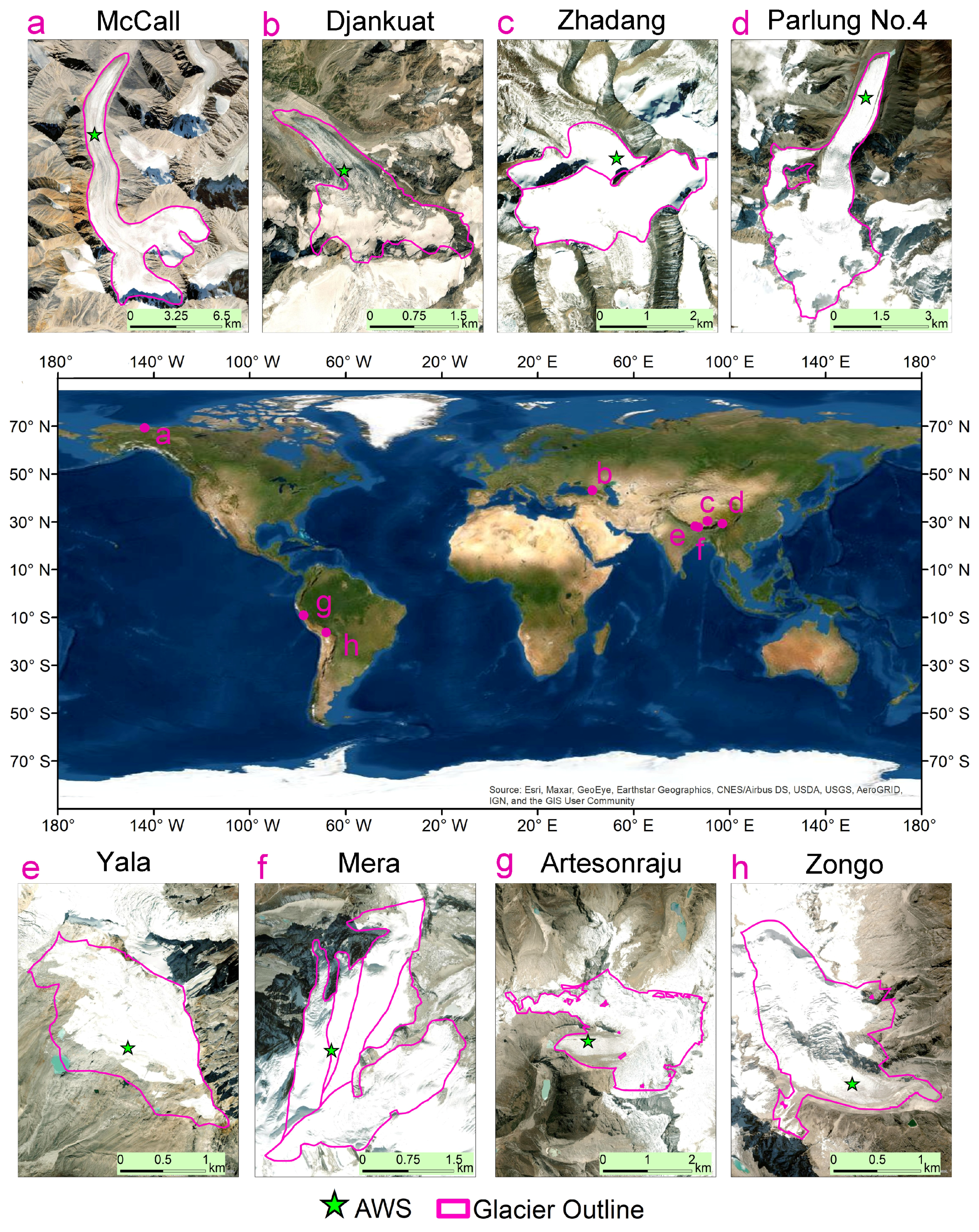
2.1. Study Sites
2.2. Datasets

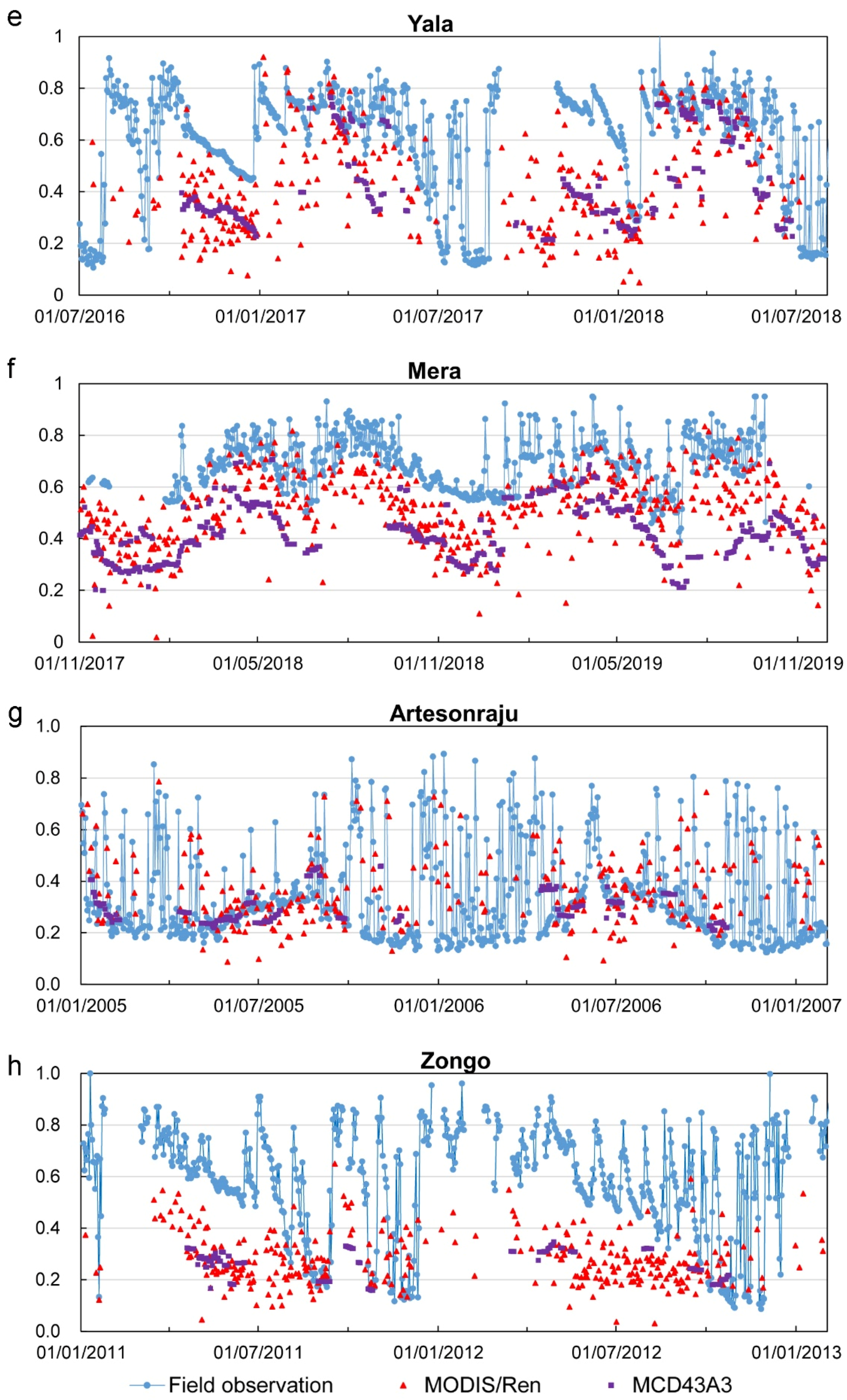
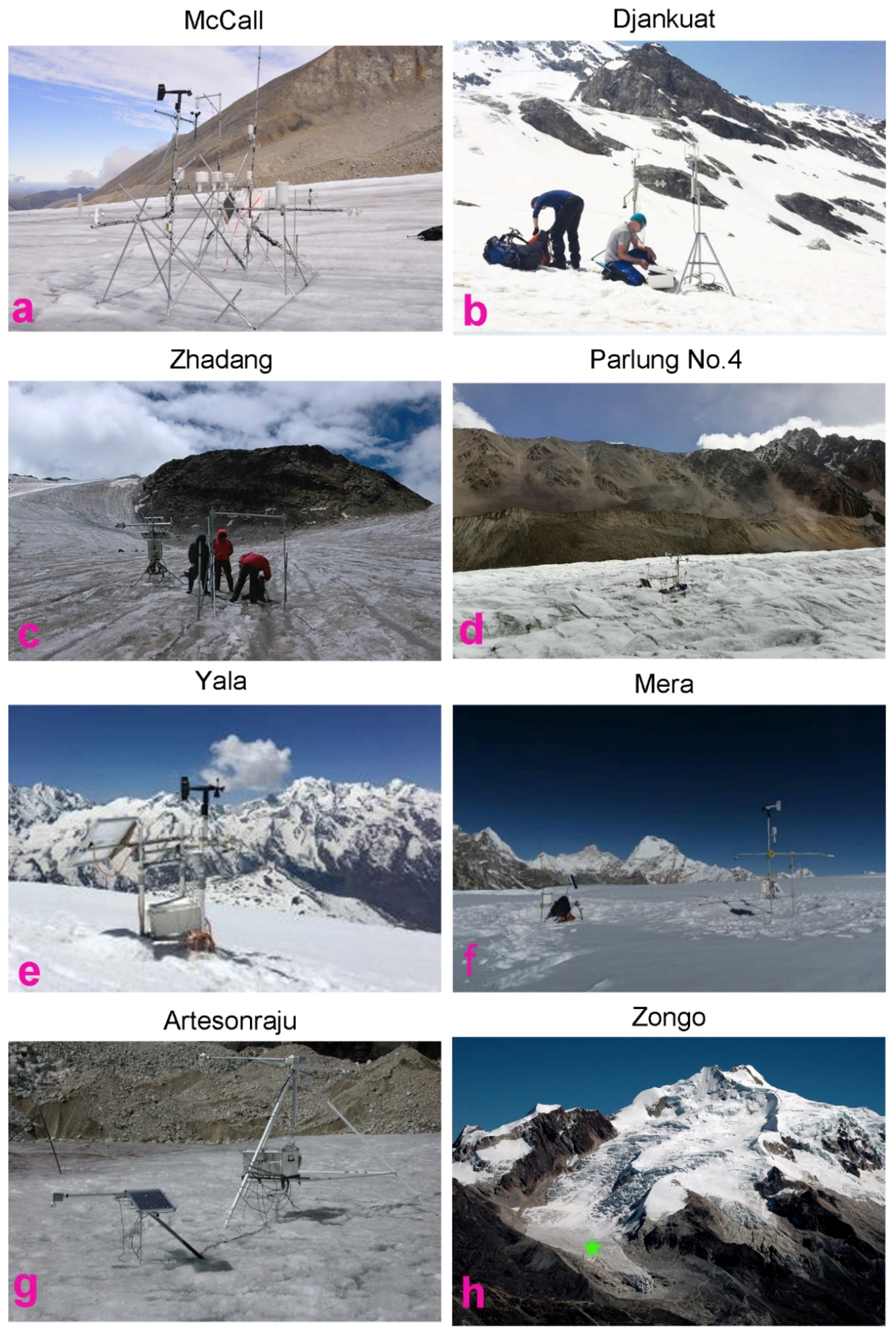
| Region | Glacier | Longitude (°) | Latitude (°) | Start Date, End Date | Elevation (m a.s.l.) | Satellite Data (Numbers of Available Scenes) | References |
|---|---|---|---|---|---|---|---|
| Alaska | McCall | −143.85 | 69.32 | 05/01/2007, 31/12/2014 | 1720 | L5/TM (10), MODIS | Troxler et al. [41] |
| Caucasus | * Djankuat | 42.76 | 43.20 | 15/06/2007, 01/09/2017 | 3000 | L5/TM (15), L8/OLI (12), MODIS | P Rets et al. [42] |
| Inner Tibetan Plateau and eastern Himalaya | Zhadang | 90.65 | 30.47 | 01/01/2011, 31/12/2014 | 5660 | L5/TM (15), MODIS | Zhang et al. [2,3] |
| Parlung No.4 | 96.93 | 29.25 | 05/01/2012, 20/09/2018 | 4600 | L8/OLI (36), MODIS | Yang et al. [43] | |
| Yala | 85.62 | 28.23 | 08/05/2016, 19/11/2019 | 5330 | L8/OLI (28), MODIS | ICIMOD | |
| Mera | 86.88 | 27.72 | 01/01/2017, 12/11/2019 | 5769 | L8/OLI (11), MODIS | GLACIOCLIM | |
| Andes | Artesonraju | −77.64 | −8.96 | 13/03/2004, 13/05/2013 | 4797 | L5/TM (13), MODIS | Winkler et al. [44] |
| Zongo | −68.14 | −16.28 | 06/08/2004, 31/08/2019 | 5050 | L5/TM (24), L8/OLI (18), MODIS | GLACIOCLIM |
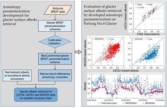
3. Methods
3.1. Anisotropy Correction of the Glacier Surface
3.2. Narrowband to Broadband Albedo Conversion
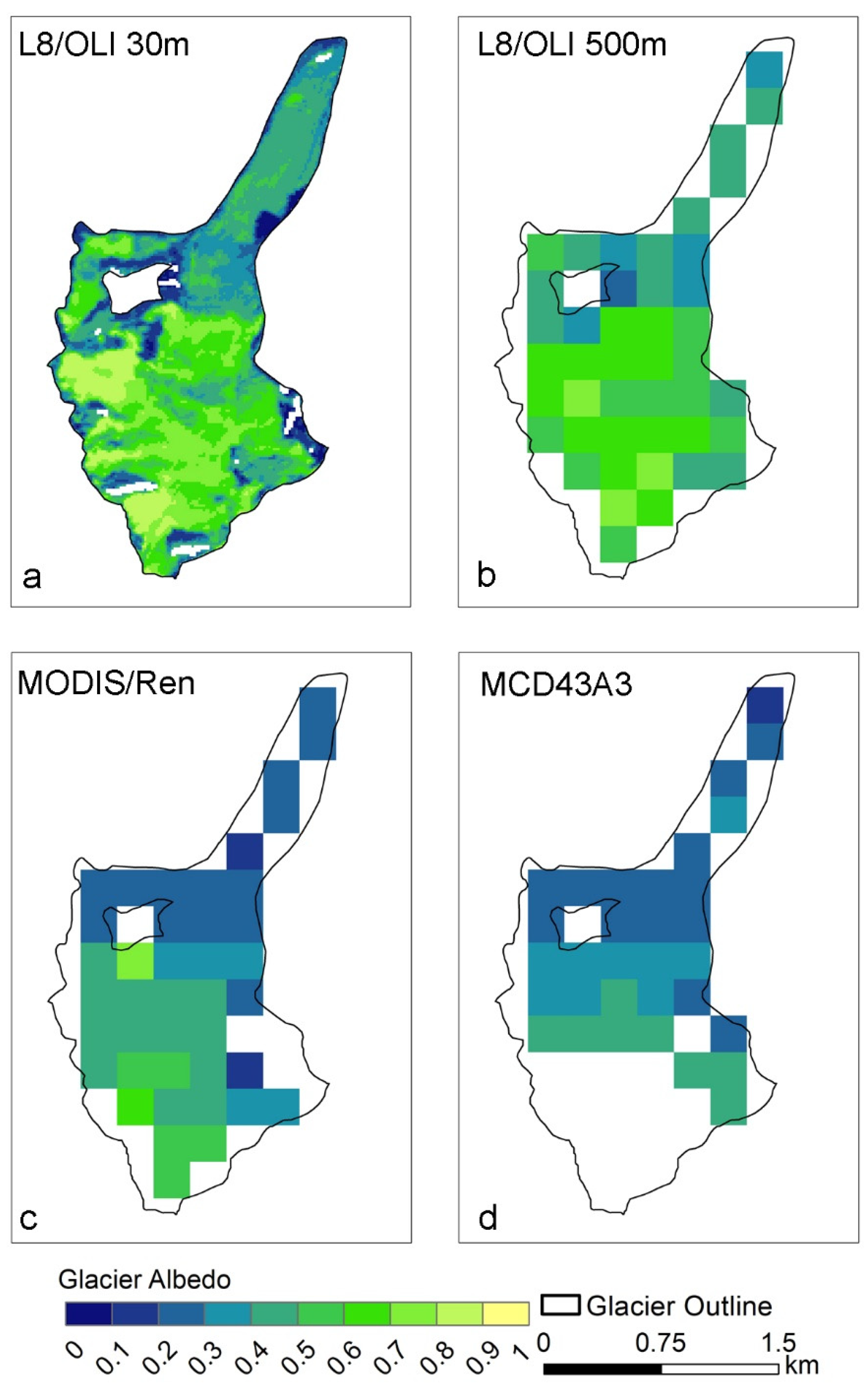
3.3. Glacier Surface Classification and Albedo Validation
4. Results
4.1. Evaluation of the Anisotropy Corrections
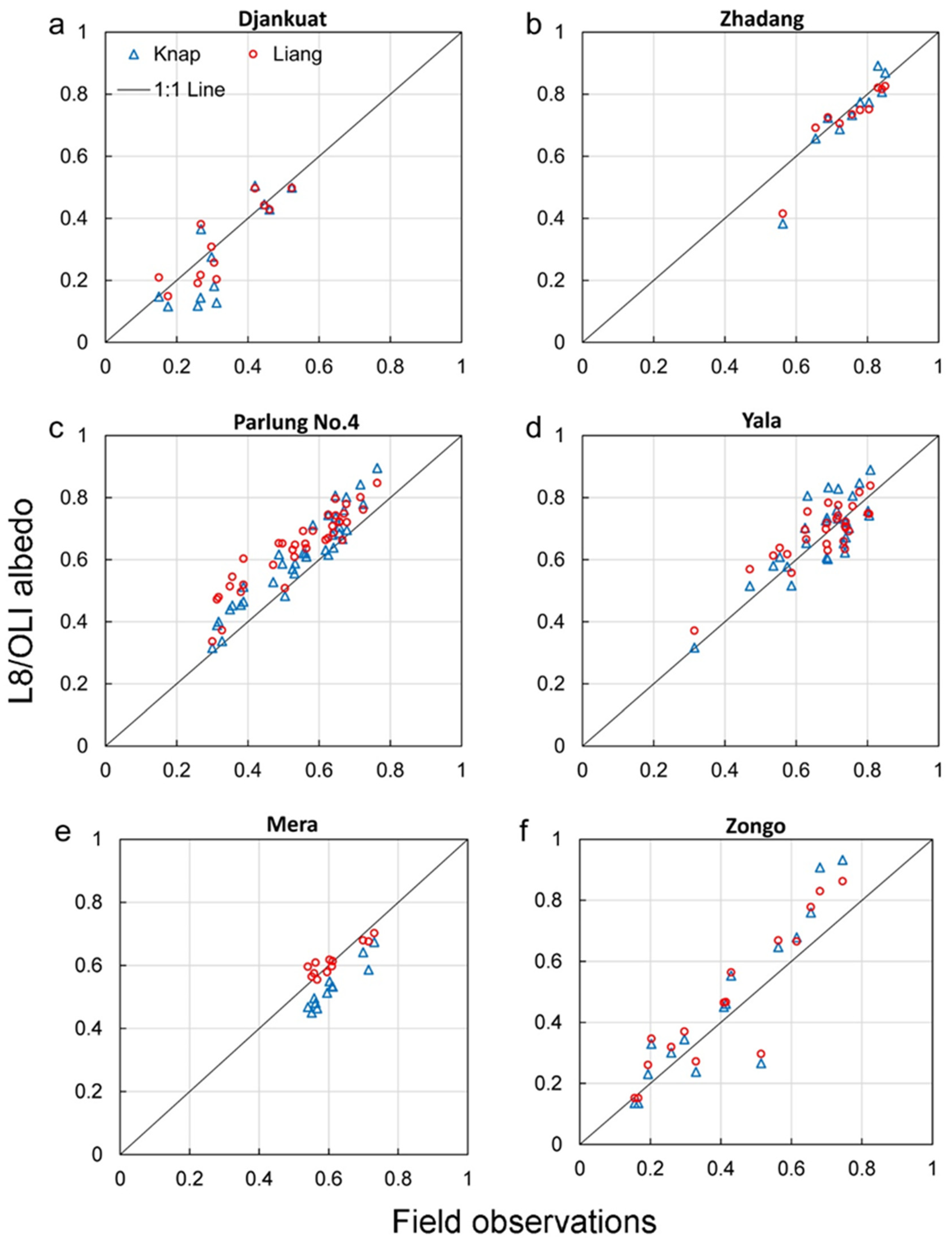
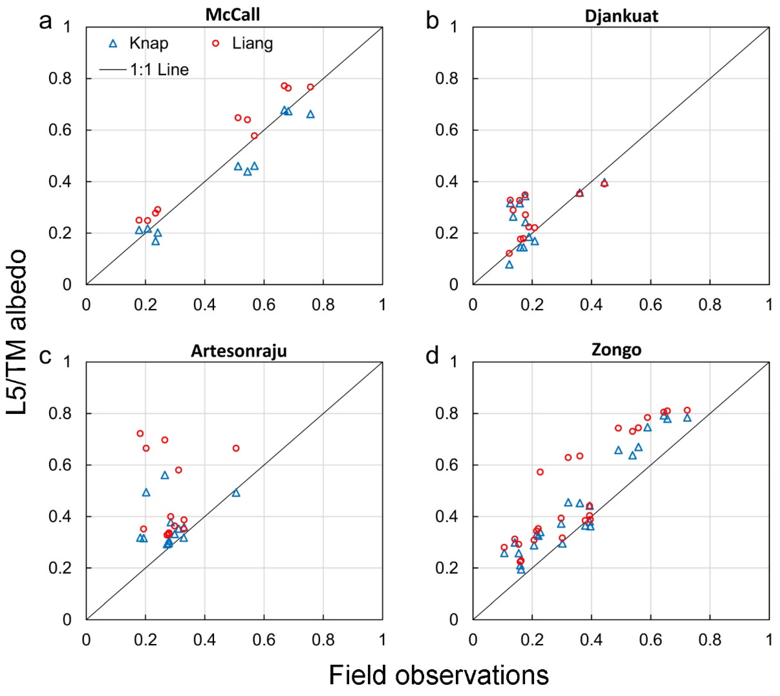
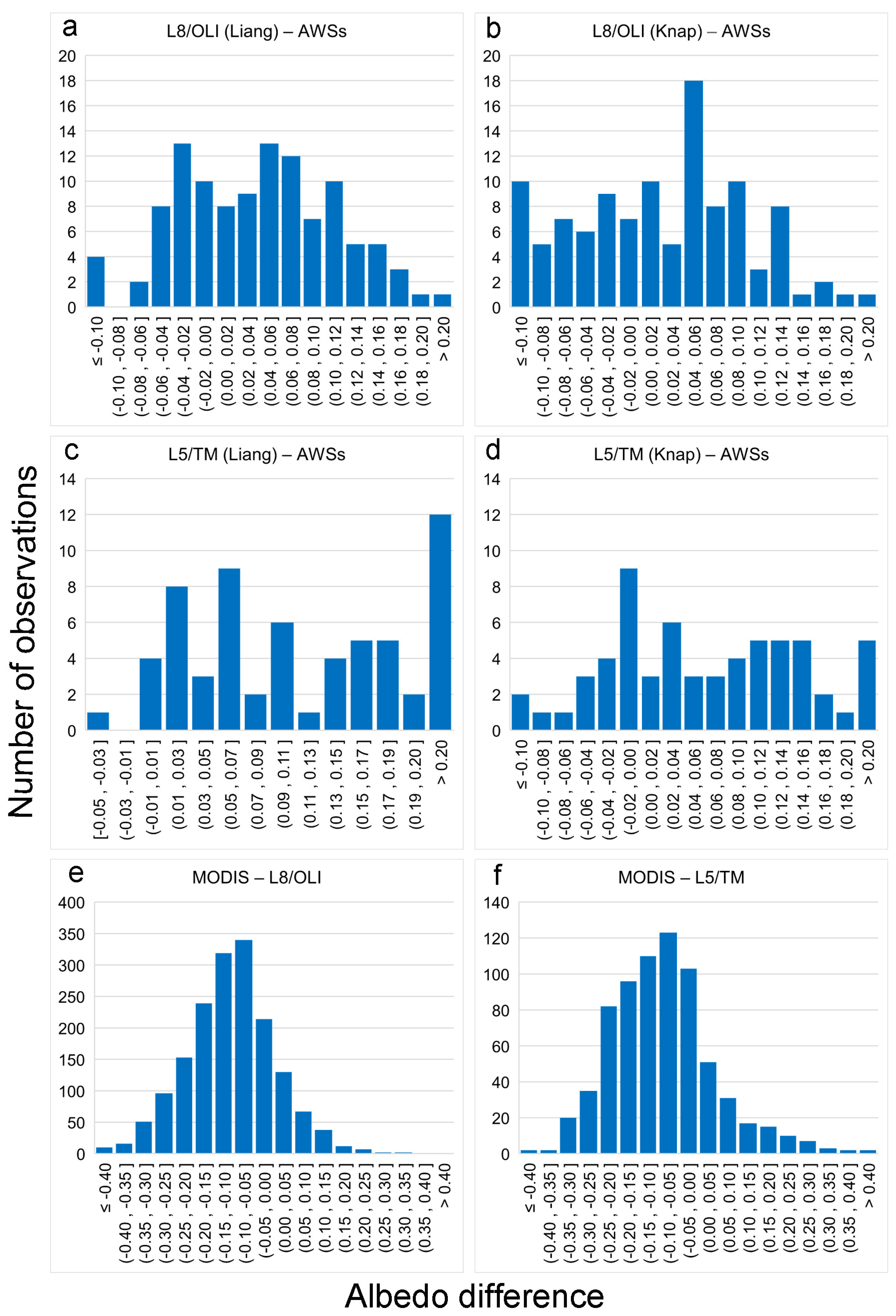
4.2. Accuracy of L8/OLI and L5/TM Albedo
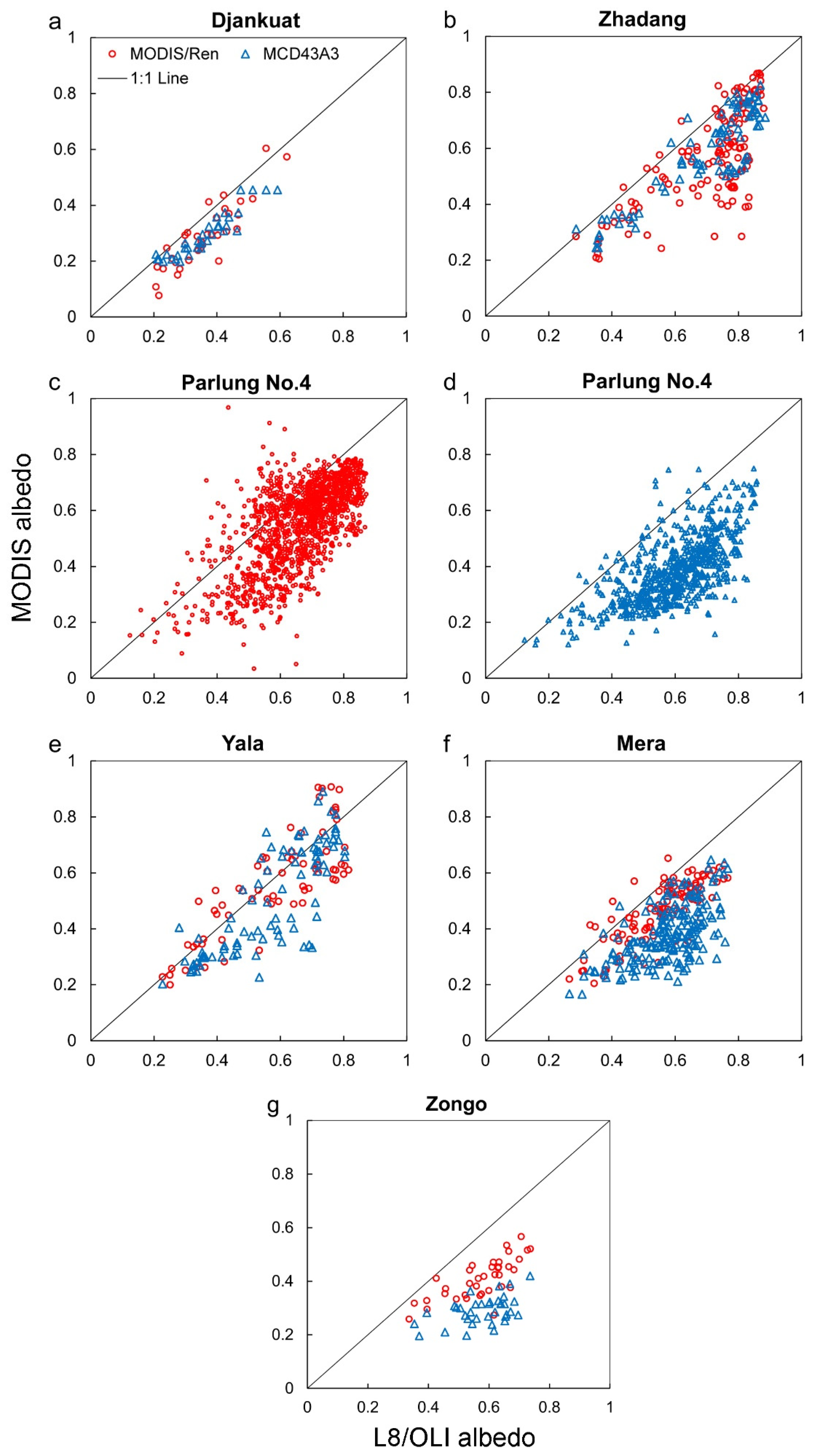
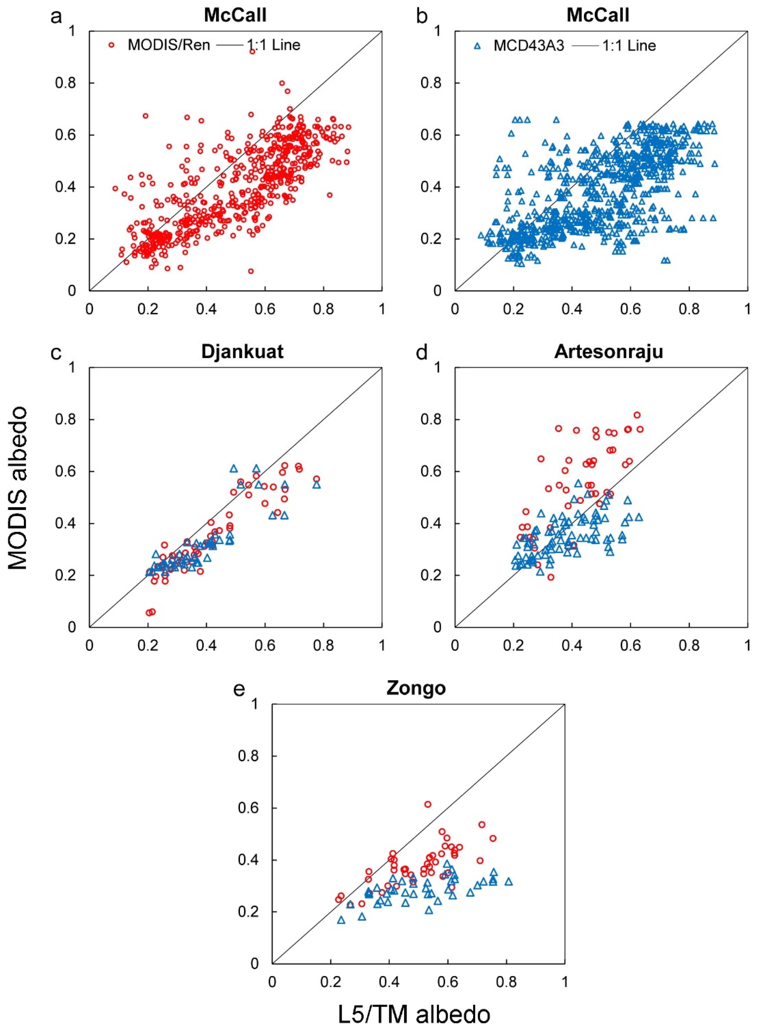
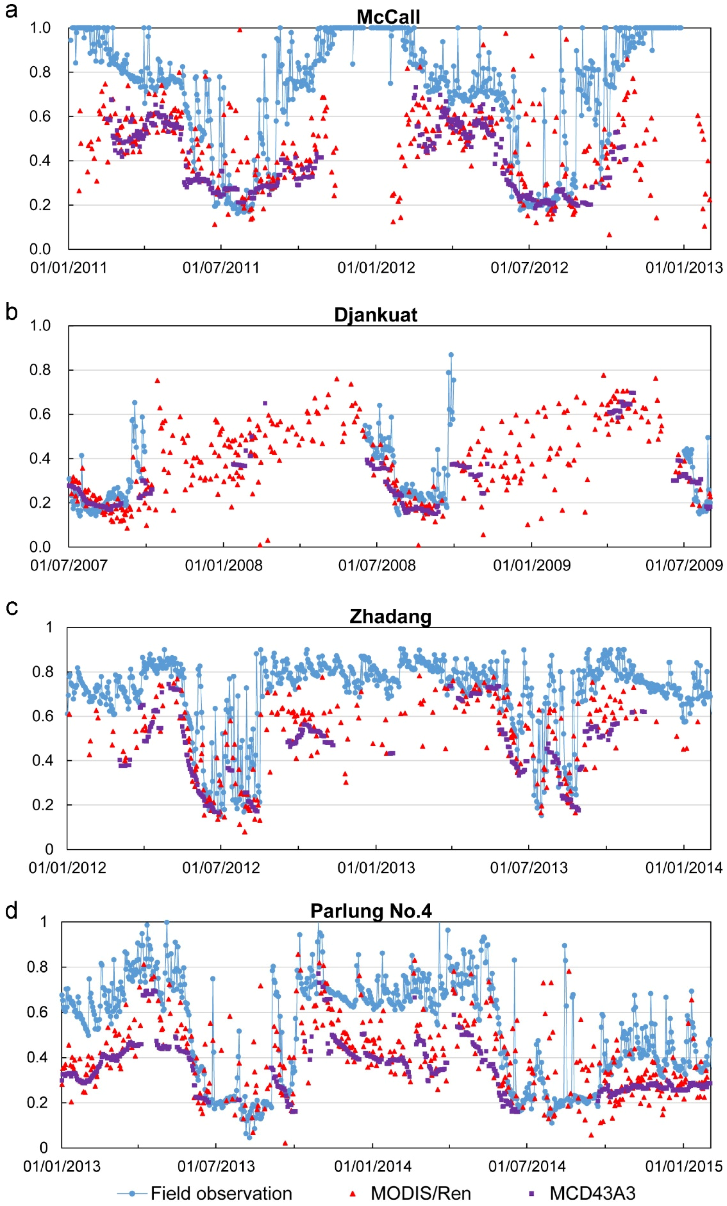
4.3. Performance of Our MODIS Albedo Product and MCD43A3
5. Discussion
5.1. Limitations of the Updated Albedo Retrieval Method
5.2. Evaluation of the Albedo Products
5.3. Potential and Future Applications of the Updated Albedo Retrieval Method
6. Conclusions
Author Contributions
Funding
Acknowledgments
Conflicts of Interest
Appendix A

| Glacier Surface | Airborne BRDF | L5/TM | L8/OLI | MODIS |
|---|---|---|---|---|
| Snow | 339 (330–350) | |||
| 382 (370–390) | ||||
| 480 (450–495) | band 1 (450–515) | band 2 (450–515) | band 3 (459–479) | |
| 677 (650–720) | band 3 (630–690) | band 4 (630–680) | band 1 (620–672) | |
| 873 (835–910) | band 4 (750–900) | band 5 (845–885) | band 2 (841–890) | |
| 1032 (990–1075) | ||||
| 1222 (1184–1258) | band 5 (1230–1250) | |||
| 1275 (1236–1319) | ||||
| 1649 (1600–1709) | band 5 (1550–1750) | band 6 (1560–1660) | ||
| 2196 (2140–2260) | band 7 (2090–2350) | band 7 (2100–2300) | band 7 (2105–2155) | |
| Ice | 471 (462–482) | band 1 (450–515) | band 2 (450–515) | band 3 (459–479) |
| 675 (665–684) | band 3 (630–690) | band 4 (630–680) | band 1 (620–672) | |
| 868 (858–877) | band 4 (750–900) | band 5 (845–885) | band 2 (841–890) | |
| 1037 (1028–1047) | ||||
| 1219 (1209–1229) | band 5 (1230–1250) | |||
| 1271 (1260–1281) | ||||
| 560 (520–600) | band 4 (545–565) |


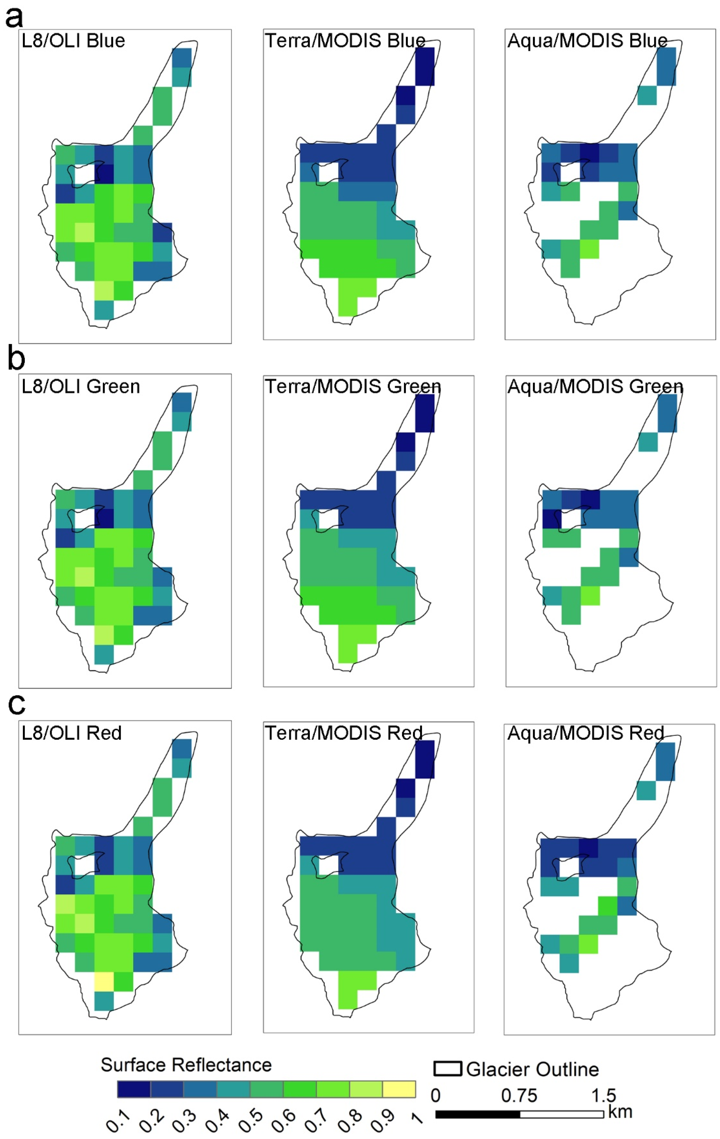
| Band Name | Range | Difference | |||
|---|---|---|---|---|---|
| L8/OLI | Terra/MODIS | Aqua/MODIS | Terra/MODIS-L8/OLI | Aqua/MODIS-L8/OLI | |
| Blue | 0.16–0.89 | 0.17–0.72 | 0.14–0.70 | −0.09 | −0.08 |
| Green | 0.19–0.90 | 0.18–0.77 | 0.16–0.73 | −0.08 | −0.08 |
| Red | 0.21–0.90 | 0.17–0.75 | 0.13–0.72 | −0.1 | −0.09 |
References
- Cuffey, K.M.; Paterson, W.S.B. The Physics of Glaciers, 4th ed.; Academic Press: Cambridge, MA, USA, 2010; ISBN 9780123694614. [Google Scholar]
- Zhang, G.S.; Kang, S.C.; Fujita, K.; Huintjes, E.; Xu, J.Q.; Yamazaki, T.; Haginoya, S.; Wei, Y.; Scherer, D.; Schneider, C.; et al. Energy and Mass Balance of Zhadang Glacier Surface, Central Tibetan Plateau. J. Glaciol. 2013, 59, 137–148. [Google Scholar] [CrossRef]
- Zhang, G.S.; Kang, S.C.; Cuo, L.; Qu, B. Modeling Hydrological Process in a Glacier Basin on the Central Tibetan Plateau with a Distributed Hydrology Soil Vegetation Model. J. Geophys. Res. 2016, 121, 9521–9539. [Google Scholar] [CrossRef]
- Olson, M.; Rupper, S.; Shean, D.E. Terrain Induced Biases in Clear-Sky Shortwave Radiation Due to Digital Elevation Model Resolution for Glaciers in Complex Terrain. Front. Earth Sci. 2019, 7, 1–12. [Google Scholar] [CrossRef]
- Nicholson, L.I.; Prinz, R.; Mölg, T.; Kaser, G. Micrometeorological Conditions and Surface Mass and Energy Fluxes on Lewis Glacier, Mt Kenya, in Relation to Other Tropical Glaciers. Cryosphere 2013, 7, 1205–1225. [Google Scholar] [CrossRef]
- Zhang, Y.; Qin, X.; Li, X.; Zhao, J.; Liu, Y. Estimation of Shortwave Solar Radiation on Clear-Sky Days for a Valley Glacier with Sentinel-2 Time Series. Remote Sens. 2020, 12, 927. [Google Scholar] [CrossRef]
- Liang, L.; Cuo, L.; Liu, Q. The Energy and Mass Balance of a Continental Glacier: Dongkemadi Glacier in Central Tibetan Plateau. Sci. Rep. 2018, 8, 1–8. [Google Scholar]
- Zhang, Z.; Jiang, L.; Liu, L.; Sun, Y.; Wang, H. Annual Glacier-Wide Mass Balance (2000–2016) of the Interior Tibetan Plateau Reconstructed from MODIS Albedo Products. Remote Sens. 2018, 10, 1031. [Google Scholar] [CrossRef]
- Brun, F.; Dumont, M.; Wagnon, P.; Berthier, E.; Azam, M.F.; Shea, J.M.; Sirguey, P.; Rabatel, A.; Ramanathan, A. Seasonal Changes in Surface Albedo of Himalayan Glaciers from MODIS Data and Links with the Annual Mass Balance. Cryosphere 2015, 9, 341–355. [Google Scholar] [CrossRef]
- Dumont, M.; Gardelle, J.; Sirguey, P.; Guillot, A.; Six, D.; Rabatel, A.; Arnaud, Y. Linking Glacier Annual Mass Balance and Glacier Albedo Retrieved from MODIS Data. Cryosphere 2012, 6, 1527–1539. [Google Scholar] [CrossRef]
- Fugazza, D.; Senese, A.; Azzoni, R.S.; Maugeri, M.; Maragno, D.; Diolaiuti, G.A. New Evidence of Glacier Darkening in the Ortles-Cevedale Group from Landsat Observations. Glob. Planet. Chang. 2019, 178, 35–45. [Google Scholar] [CrossRef]
- Naegeli, K.; Huss, M.; Hoelzle, M. Change Detection of Bare-Ice Albedo in the Swiss Alps. Cryosphere 2019, 13, 397–412. [Google Scholar] [CrossRef]
- Shaw, T.E.; Ulloa, G.; Farías-Barahona, D.; Fernandez, R.; Lattus, J.M.; McPhee, J. Glacier Albedo Reduction and Drought Effects in the Extratropical Andes, 1986–2020. J. Glaciol. 2021, 67, 158–169. [Google Scholar] [CrossRef]
- Qu, Y.; Liang, S.; Liu, Q.; He, T.; Liu, S.; Li, X. Mapping Surface Broadband Albedo from Satellite Observations: A Review of Literatures on Algorithms and Products. Remote Sens. 2015, 7, 990–1020. [Google Scholar] [CrossRef]
- Schaaf, C.B.; Gao, F.; Strahler, A.H.; Lucht, W.; Li, X.; Tsang, T.; Strugnell, N.C.; Zhang, X.; Jin, Y.; Muller, J.; et al. First Operational BRDF, Albedo Nadir Reflectance Products from MODIS. Remote Sens. Environ. 2002, 83, 135–148. [Google Scholar] [CrossRef]
- Masek, J.G.; Vermote, E.F.; Saleous, N.E.; Wolfe, R.; Hall, F.G.; Huemmrich, K.F.; Gao, F.; Kutler, J.; Lim, T.K. A Landsat Surface Reflectance Dataset for North America, 1990–2000. IEEE Geosci. Remote Sens. Lett. 2006, 3, 68–72. [Google Scholar] [CrossRef]
- Vermote, E.; Justice, C.; Claverie, M.; Franch, B. Preliminary Analysis of the Performance of the Landsat 8/OLI Land Surface Reflectance Product. Remote Sens. Environ. 2016, 185, 46–56. [Google Scholar] [CrossRef]
- Knap, W.H.; Reijmer, C.H.; Oerlemans, J. Narrowband to Broadband Conversion of Landsat tm Glacier Albedos. Int. J. Remote Sens. 1999, 20, 2091–2110. [Google Scholar] [CrossRef]
- Liang, S.L. Narrowband to Broadband Conversions of Land Surface Albedo I Algorithms. Remote Sens. Environ. 2001, 76, 213–238. [Google Scholar] [CrossRef]
- Stroeve, J.; Box, J.E.; Gao, F.; Liang, S.; Nolin, A.; Schaaf, C. Accuracy Assessment of the MODIS 16-day Albedo Product for Snow: Comparisons with Greenland in Situ Measurements. Remote Sens. Environ. 2005, 94, 46–60. [Google Scholar] [CrossRef]
- Lucht, W.; Schaaf, C.B.; Strahler, A.H. An Algorithm for the Retrieval of Albedo from Space Using Semiempirical BRDF Models. IEEE Trans. Geosci. Remote Sens. 2000, 38, 977–998. [Google Scholar] [CrossRef]
- Reijmer, C.H.; Bintanja, R.; Greuell, W. Surface Albedo Measurements over Snow and Blue Ice in Thematic Mapper Bands 2 and 4 in Dronning Maud Land, Antarctica. J. Geophys. Res. 2001, 106, 9661–9672. [Google Scholar] [CrossRef]
- Greuell, W.; De Ruyter De Wildt, M. Anisotropic Reflection by Melting Glacier Ice: Measurements and Parametrizations in Landsat TM bands 2 and 4. Remote Sens. Environ. 1999, 70, 265–277. [Google Scholar] [CrossRef]
- Wang, J.; Ye, B.S.; Cui, Y.H.; He, X.B.; Yang, G.J. Spatial and Temporal Variations of Albedo on Nine Glaciers in Western China from 2000 to 2011. Hydrol. Process. 2014, 28, 3454–3465. [Google Scholar] [CrossRef]
- Pope, A.; Rees, W.G. Impact of Spatial, Spectral, and Radiometric Properties of Multispectral Imagers on Glacier Surface Classification. Remote Sens. Environ. 2014, 141, 1–13. [Google Scholar] [CrossRef]
- Pope, E.L.; Willis, I.C.; Pope, A.; Miles, E.S.; Arnold, N.S.; Rees, W.G. Contrasting Snow and Ice Albedos Derived from MODIS, Landsat ETM+ and Airborne Data from Langjökull, Iceland. Remote Sens. Environ. 2016, 175, 183–195. [Google Scholar] [CrossRef]
- Klok, E.J.; Greuell, W.; Oerlemans, J. Temporal and Spatial Variation of the Surface Albedo of Morteratschgletscher, Switzerland, as Derived from 12 Landsat Images. J. Glaciol. 2004, 49, 491–502. [Google Scholar] [CrossRef]
- Naegeli, K.; Damm, A.; Huss, M.; Wulf, H.; Schaepman, M.; Hoelzle, M. Cross-Comparison of Albedo Products for Glacier Surfaces Derived from Airborne and Satellite (Sentinel-2 and Landsat 8) Optical Data. Remote Sens. 2017, 9, 110. [Google Scholar] [CrossRef]
- Kaspari, S.; Painter, T.H.; Gysel, M.; Skiles, S.M.; Schwikowski, M. Seasonal and Elevational Variations of Black Carbon and Dust in Snow and Ice in the Solu-Khumbu, Nepal and Estimated Radiative Forcings. Atmos. Chem. Phys. 2014, 14, 8089–8103. [Google Scholar] [CrossRef]
- Williamson, S.N.; Copland, L.; Thomson, L.; Burgess, D. Comparing Simple Albedo Scaling Methods for Estimating Arctic Glacier Mass Balance. Remote Sens. Environ. 2020, 246, 111858. [Google Scholar] [CrossRef]
- Gatebe, C.K.; King, M.D. Airborne Spectral BRDF of Various Surface Types (Ocean, Vegetation, Snow, Desert, Wetlands, Cloud Decks, Smoke Layers) for Remote Sensing Applications. Remote Sens. Environ. 2016, 179, 131–148. [Google Scholar] [CrossRef]
- Naegeli, K.; Damm, A.; Huss, M.; Schaepman, M.; Hoelzle, M. Imaging Spectroscopy to Assess the Composition of Ice Surface Materials and their Impact on Glacier Mass Balance. Remote Sens. Environ. 2015, 168, 388–402. [Google Scholar] [CrossRef]
- Dumont, M.; Brissaud, O.; Picard, G.; Schmitt, B.; Gallet, J.C.; Arnaud, Y. High-Accuracy Measurements of Snow Bidirectional Reflectance Distribution Function at Visible and NIR Wavelengths-Comparison with Modelling Results. Atmos. Chem. Phys. 2010, 10, 2507–2520. [Google Scholar] [CrossRef]
- Lyapustin, A.; Gatebe, C.K.; Kahn, R.; Brandt, R.; Redemann, J.; Russell, P.; King, M.D.; Pedersen, C.A.; Gerland, S.; Poudyal, R.; et al. Analysis of Snow Bidirectional Reflectance from ARCTAS Spring-2008 Campaign. Atmos. Chem. Phys. 2010, 10, 4359–4375. [Google Scholar] [CrossRef]
- Perovich, D.K. Complex yet Translucent: The Optical Properties of Sea Ice. Phys. B Condens. Matter 2003, 338, 107–114. [Google Scholar] [CrossRef]
- Warren, S.G. Optical Properties of Ice and Snow. Philos. Trans. R. Soc. A Math. Phys. Eng. Sci. 2019, 377, 20180161. [Google Scholar] [CrossRef]
- Yue, X.; Li, Z.; Zhao, J.; Fan, J.; Takeuchi, N.; Wang, L. Variation in Albedo and Its Relationship With Surface Dust at Urumqi Glacier No. 1 in Tien Shan, China. Front. Earth Sci. 2020, 8, 1–14. [Google Scholar] [CrossRef]
- Wang, X.; Zender, C.S. Arctic and Antarctic Diurnal and Seasonal Variations of Snow Albedo from Multiyear Baseline Surface Radiation Network Measurements. J. Geophys. Res. Earth Surf. 2011, 116, 1–16. [Google Scholar] [CrossRef]
- Mortimer, C.A.; Sharp, M. Spatiotemporal Variability of Canadian High Arctic Glacier Surface Albedo from MODIS Data, 2001–2016. Cryosphere 2018, 12, 701–720. [Google Scholar] [CrossRef]
- Tadono, T.; Ishida, H.; Oda, F.; Naito, S.; Minakawa, K.; Iwamoto, H. Precise Global DEM Generation by ALOS PRISM. ISPRS Ann. Photogramm. Remote Sens. Spat. Inf. Sci. 2014, II–4, 71–76. [Google Scholar] [CrossRef]
- Troxler, P.; Ayala, Á.; Shaw, T.E.; Nolan, M.; Brock, B.W.; Pellicciotti, F. Modelling Spatial Patterns of Near-Surface Air Temperature over a Decade of Melt Seasons on McCall Glacier, Alaska. J. Glaciol. 2020, 66, 386–400. [Google Scholar] [CrossRef]
- Rets, E.P.; Popovnin, V.V.; Toropov, P.A.; Smirnov, A.M.; Tokarev, I.V.; Chizhova, J.N.; Budantseva, N.A.; Vasil’Chuk, Y.K.; Kireeva, M.B.; Ekaykin, A.A.; et al. Djankuat Glacier Station in the North Caucasus, Russia: A Database of Glaciological, Hydrological, and Meteorological Observations and Stable Isotope Sampling Results During 2007–2017. Earth Syst. Sci. Data 2019, 11, 1463–1481. [Google Scholar] [CrossRef]
- Yang, W.; Guo, X.; Yao, T.; Yang, K.; Zhao, L.; Li, S.; Zhu, M. Summertime Surface Energy Budget and Ablation Modeling in the Ablation Zone of a Maritime Tibetan Glacier. J. Geophys. Res. Atmos. 2011, 116, 1–11. [Google Scholar] [CrossRef]
- Winkler, M.; Juen, I.; Mölg, T.; Wagnon, P.; Gómez, J.; Kaser, G. Measured and Modelled Sublimation on the Tropical Glaciar Artesonraju, Perú. Cryosphere 2009, 3, 21–30. [Google Scholar] [CrossRef]
- Warren, S.G.; Brandt, R.E.; Hinton, P.O.R. Effect of Surface Roughness on Bidirectional Reflectance of Antarctic Snow. J. Geophys. Res. E Planets 1998, 103, 25789–25807. [Google Scholar] [CrossRef]
- Knap, W.H.; Reijmer, C.H. Anisotropy of the Reflected Radiation Field over Melting Glacier Ice: Measurements in Landsat TM Bands 2 and 4. Remote Sens. Environ. 1998, 65, 93–104. [Google Scholar] [CrossRef]
- Wen, J.; Liu, Q.; Liu, Q.; Xiao, Q.; Li, X. Parametrized BRDF for Atmospheric and Topographic Correction and Albedo Estimation in Jiangxi Rugged Terrain, China. Int. J. Remote Sens. 2009, 30, 2875–2896. [Google Scholar] [CrossRef]
- Yue, X.Y.; Zhao, J.; Li, Z.Q.; Zhang, M.J.; Fan, J.; Wang, L.; Wang, P.Y. Spatial and Temporal Variations of the Surface Albedo and Other Factors Influencing Urumqi Glacier No. 1 in Tien Shan, China. J. Glaciol. 2017, 63, 899–911. [Google Scholar] [CrossRef]
- Wen, J.G.; Liu, Q.H.; Xiao, Q.; Liu, Q.; Li, X.W. Modeling the Land Surface Reflectance for Optical Remote Sensing Data in Rugged Terrain. Sci. China Ser. D Earth Sci. 2008, 51, 1169–1178. [Google Scholar] [CrossRef]
- Gardner, A.S.; Sharp, M.J. A Review of Snow and Ice Albedo and the Development of a New Physically Based Broadband Albedo Parameterization. J. Geophys. Res. Earth Surf. 2010, 115, 1–15. [Google Scholar] [CrossRef]
- Girona-Mata, M.; Miles, E.S.; Ragettli, S.; Pellicciotti, F. High-Resolution Snowline Delineation From Landsat Imagery to Infer Snow Cover Controls in a Himalayan Catchment. Water Resour. Res. 2019, 55, 6754–6772. [Google Scholar] [CrossRef]
- Härer, S.; Bernhardt, M.; Siebers, M.; Schulz, K. On the Need for a Time- and Location-Dependent Estimation of the NDSI Threshold Value for Reducing Existing Uncertainties in Snow Cover Maps at Different Scales. Cryosphere 2018, 12, 1629–1642. [Google Scholar] [CrossRef]
- Roupioz, L.; Nerry, F.; Jia, L.; Menenti, M. Improved Surface Reflectance from Remote Sensing Data with Sub-Pixel Topographic Information. Remote Sens. 2014, 6, 10356–10374. [Google Scholar] [CrossRef]
- Moustafa, S.E.; Rennermalm, A.K.; Román, M.O.; Wang, Z.; Schaaf, C.B.; Smith, L.C.; Koenig, L.S.; Erb, A. Evaluation of Satellite Remote Sensing Albedo Retrievals over the Ablation Area of the Southwestern Greenland Ice Sheet. Remote Sens. Environ. 2017, 198, 115–125. [Google Scholar] [CrossRef]
- Manninen, T.; Anttila, K.; Jääskeläinen, E.; Riihelä, A.; Peltoniemi, J.; Räisänen, P.; Lahtinen, P.; Siljamo, N.; Thölix, L.; Meinander, O.; et al. Effect of Small-Scale Snow Surface Roughness on Snow Albedo and Reflectance. Cryosph. Discuss. 2020, 1–56. [Google Scholar]
- Arnold, N.S.; Rees, W.G.; Hodson, A.J.; Kohler, J. Topographic Controls on the Surface Energy Balance of a High Arctic Valley Glacier. J. Geophys. Res. Earth Surf. 2006, 111, 1–15. [Google Scholar] [CrossRef]
- Lhermitte, S.; Abermann, J.; Kinnard, C. Albedo Over Rough Snow and Ice Surfaces. Cryosphere 2014, 8, 1069–1086. [Google Scholar] [CrossRef]


| Experiment | BRDF Parameterization | |||
|---|---|---|---|---|
| P1 | ||||
| * P2 | ||||
| P3 | ||||
| P4 | ||||
| Glacier Surface | Parameterization Scheme | Calibration | Validation | ||||
|---|---|---|---|---|---|---|---|
| R | MD | Std | R | MD | Std | ||
| Snow | P1 | 0.935 | 0.0034 | 0.0736 | 0.939 | 0.0031 | 0.0726 |
| P2 | 0.935 | 0.0040 | 0.0742 | 0.938 | 0.0036 | 0.0732 | |
| P3 | 0.931 | 0.0047 | 0.0768 | 0.935 | 0.0044 | 0.0757 | |
| P4 | 0.883 | 0.0091 | 0.1076 | 0.887 | 0.0087 | 0.1064 | |
| Ice | P1 | 0.796 | −0.0008 | 0.0807 | 0.815 | 0.0011 | 0.0796 |
| P2 | 0.798 | −0.0009 | 0.0805 | 0.817 | 0.0012 | 0.0792 | |
| P3 | 0.799 | −0.0008 | 0.0803 | 0.817 | 0.0013 | 0.0791 | |
| P4 | 0.794 | −0.0003 | 0.0821 | 0.811 | 0.0022 | 0.0809 | |
| Glacier Surface | Airborne BRDF Dataset | ||||||||||
|---|---|---|---|---|---|---|---|---|---|---|---|
| Central (Range) Wavelength (nm) | Weighting Coefficients | Calibration | Validation | ||||||||
| c1 | c2 | c3 | R | MD | Std | R | MD | Std | |||
| Snow | 339 (330–350) | 0.00514 | 0.00494 | 0.01585 | 1.57080 | 0.91 | 0.0001 | 0.014 | 0.93 | 0.0000 | 0.012 |
| 382 (370–390) | 0.00189 | 0.01029 | 0.02096 | 1.01490 | 0.91 | 0.0005 | 0.019 | 0.92 | 0.0005 | 0.018 | |
| 480 (450–495) | 0.00000 | 0.00001 | 0.00002 | 0.12131 | 0.76 | 0.0078 | 0.188 | 0.77 | 0.0057 | 0.187 | |
| 677 (650–720) | 0.00083 | 0.00384 | 0.00452 | 0.34527 | 0.95 | 0.0013 | 0.034 | 0.95 | 0.0010 | 0.033 | |
| 873 (835–910) | 0.00123 | 0.00459 | 0.00521 | 0.34834 | 0.96 | 0.0015 | 0.038 | 0.96 | 0.0013 | 0.037 | |
| 1032 (990–1075) | 0.00417 | 0.00709 | 0.00736 | 0.39306 | 0.97 | 0.0014 | 0.042 | 0.97 | 0.0010 | 0.041 | |
| 1222 (1184–1258) | 0.00663 | 0.01081 | 0.01076 | 0.46132 | 0.98 | 0.0021 | 0.051 | 0.98 | 0.0017 | 0.050 | |
| 1275 (1236–1319) | 0.00413 | 0.00954 | 0.01018 | 0.46048 | 0.97 | 0.0022 | 0.061 | 0.97 | 0.0019 | 0.059 | |
| 1649 (1600–1709) | 0.00798 | 0.01744 | 0.01680 | 0.63119 | 0.96 | 0.0083 | 0.156 | 0.96 | 0.0091 | 0.163 | |
| 2196 (2140–2260) | 0.00622 | 0.01410 | 0.01314 | 0.55261 | 0.97 | 0.0093 | 0.133 | 0.98 | 0.0087 | 0.125 | |
| Ice | 471 (462–482) | −0.00369 | 0.00000 | 0.00007 | 0.27632 | 0.70 | 0.0119 | 0.045 | 0.72 | 0.0133 | 0.043 |
| 675 (665–684) | −0.00054 | 0.00002 | 0.00001 | 0.17600 | 0.71 | 0.0075 | 0.053 | 0.74 | 0.0099 | 0.051 | |
| 868 (858–877) | −0.00924 | 0.00033 | −0.00005 | 0.31750 | 0.82 | 0.0051 | 0.060 | 0.85 | 0.0073 | 0.057 | |
| 1037 (1028–1047) | −0.03533 | 0.00297 | −0.00032 | 0.54050 | 0.87 | 0.0003 | 0.080 | 0.89 | 0.0024 | 0.077 | |
| 1219 (1209–1229) | −0.02388 | 0.00656 | 0.00227 | 0.58473 | 0.84 | −0.0127 | 0.117 | 0.85 | −0.0091 | 0.117 | |
| 1271 (1260–1281) | −0.02081 | 0.00683 | 0.00390 | 0.57552 | 0.84 | −0.0176 | 0.128 | 0.84 | −0.0168 | 0.131 | |
| * 560 (520–600) | −0.02920 | −0.00810 | 0.00462 | 0.52360 | / | / | 0.043 | / | / | / | |
| Satellite | Glacier | n | Field Observation | Knap Method | Liang Method | ||||||
|---|---|---|---|---|---|---|---|---|---|---|---|
| Mean | Mean | Bias | MAE | RMSE | Mean | Bias | MAE | RMSE | |||
| L8/OLI | Djankuat | 12 | 0.32 | 0.28 | −0.04 | 0.07 | 0.09 | 0.31 | −0.01 | 0.05 | 0.06 |
| Zhadang | 15 | 0.75 | 0.73 | −0.02 | 0.04 | 0.06 | 0.72 | −0.03 | 0.04 | 0.06 | |
| Parlung No.4 | 36 | 0.54 | 0.61 | 0.07 | 0.07 | 0.08 | 0.64 | 0.10 | 0.10 | 0.11 | |
| Yala | 28 | 0.67 | 0.69 | 0.01 | 0.06 | 0.07 | 0.69 | 0.01 | 0.05 | 0.06 | |
| Mera | 11 | 0.61 | 0.53 | −0.08 | 0.08 | 0.08 | 0.61 | 0.00 | 0.03 | 0.03 | |
| Zongo | 18 | 0.42 | 0.48 | 0.06 | 0.10 | 0.13 | 0.49 | 0.06 | 0.10 | 0.11 | |
| Average | / | 0.55 | 0.55 | 0.00 | 0.07 | 0.09 | 0.58 | 0.02 | 0.06 | 0.07 | |
| L5/TM | McCall | 10 | 0.46 | 0.42 | −0.04 | 0.05 | 0.06 | 0.52 | 0.06 | 0.06 | 0.07 |
| Djankuat | 15 | 0.20 | 0.28 | 0.09 | 0.11 | 0.14 | 0.33 | 0.13 | 0.14 | 0.20 | |
| Artesonraju | 13 | 0.29 | 0.39 | 0.11 | 0.11 | 0.17 | 0.47 | 0.19 | 0.19 | 0.25 | |
| Zongo | 24 | 0.36 | 0.45 | 0.09 | 0.09 | 0.10 | 0.50 | 0.14 | 0.14 | 0.17 | |
| Average | / | 0.33 | 0.39 | 0.06 | 0.09 | 0.12 | 0.46 | 0.13 | 0.13 | 0.17 | |
| Satellite | Glacier | n | MODIS/Ren | n | MCD43A3 | ||||||||
|---|---|---|---|---|---|---|---|---|---|---|---|---|---|
| MLandsat | MMODIS | Bias | MAE | RMSE | MLandsat | MMODIS | Bias | MAE | RMSE | ||||
| L8/OLI | Djankuat | 34 | 0.36 | 0.29 | −0.07 | 0.08 | 0.09 | 34 | 0.36 | 0.29 | −0.07 | 0.07 | 0.08 |
| Zhadang | 132 | 0.71 | 0.57 | −0.14 | 0.14 | 0.18 | 87 | 0.69 | 0.58 | −0.11 | 0.11 | 0.13 | |
| Parlung No.4 | 1313 | 0.66 | 0.55 | −0.11 | 0.13 | 0.16 | 671 | 0.60 | 0.39 | −0.21 | 0.22 | 0.24 | |
| Yala | 69 | 0.58 | 0.56 | −0.02 | 0.09 | 0.11 | 105 | 0.55 | 0.49 | −0.07 | 0.10 | 0.12 | |
| Mera | 112 | 0.56 | 0.47 | −0.09 | 0.10 | 0.12 | 189 | 0.58 | 0.38 | −0.20 | 0.20 | 0.22 | |
| Zongo | 37 | 0.58 | 0.41 | −0.17 | 0.17 | 0.18 | 36 | 0.58 | 0.29 | −0.29 | 0.29 | 0.30 | |
| Average | / | 0.57 | 0.47 | −0.10 | 0.12 | 0.14 | / | 0.56 | 0.40 | −0.16 | 0.16 | 0.18 | |
| L5/TM | McCall | 589 | 0.50 | 0.40 | −0.10 | 0.13 | 0.16 | 769 | 0.49 | 0.38 | −0.12 | 0.15 | 0.19 |
| Djankuat | 57 | 0.41 | 0.35 | −0.06 | 0.07 | 0.09 | 48 | 0.38 | 0.32 | −0.06 | 0.08 | 0.09 | |
| Artesonraju | 47 | 0.42 | 0.55 | 0.13 | 0.14 | 0.17 | 83 | 0.38 | 0.35 | −0.02 | 0.07 | 0.09 | |
| Zongo | 45 | 0.50 | 0.38 | −0.12 | 0.13 | 0.15 | 41 | 0.51 | 0.29 | −0.22 | 0.22 | 0.26 | |
| Average | / | 0.46 | 0.42 | −0.04 | 0.12 | 0.14 | / | 0.44 | 0.33 | −0.11 | 0.13 | 0.16 | |
Publisher’s Note: MDPI stays neutral with regard to jurisdictional claims in published maps and institutional affiliations. |
© 2021 by the authors. Licensee MDPI, Basel, Switzerland. This article is an open access article distributed under the terms and conditions of the Creative Commons Attribution (CC BY) license (https://creativecommons.org/licenses/by/4.0/).
Share and Cite
Ren, S.; Miles, E.S.; Jia, L.; Menenti, M.; Kneib, M.; Buri, P.; McCarthy, M.J.; Shaw, T.E.; Yang, W.; Pellicciotti, F. Anisotropy Parameterization Development and Evaluation for Glacier Surface Albedo Retrieval from Satellite Observations. Remote Sens. 2021, 13, 1714. https://doi.org/10.3390/rs13091714
Ren S, Miles ES, Jia L, Menenti M, Kneib M, Buri P, McCarthy MJ, Shaw TE, Yang W, Pellicciotti F. Anisotropy Parameterization Development and Evaluation for Glacier Surface Albedo Retrieval from Satellite Observations. Remote Sensing. 2021; 13(9):1714. https://doi.org/10.3390/rs13091714
Chicago/Turabian StyleRen, Shaoting, Evan S. Miles, Li Jia, Massimo Menenti, Marin Kneib, Pascal Buri, Michael J. McCarthy, Thomas E. Shaw, Wei Yang, and Francesca Pellicciotti. 2021. "Anisotropy Parameterization Development and Evaluation for Glacier Surface Albedo Retrieval from Satellite Observations" Remote Sensing 13, no. 9: 1714. https://doi.org/10.3390/rs13091714
APA StyleRen, S., Miles, E. S., Jia, L., Menenti, M., Kneib, M., Buri, P., McCarthy, M. J., Shaw, T. E., Yang, W., & Pellicciotti, F. (2021). Anisotropy Parameterization Development and Evaluation for Glacier Surface Albedo Retrieval from Satellite Observations. Remote Sensing, 13(9), 1714. https://doi.org/10.3390/rs13091714