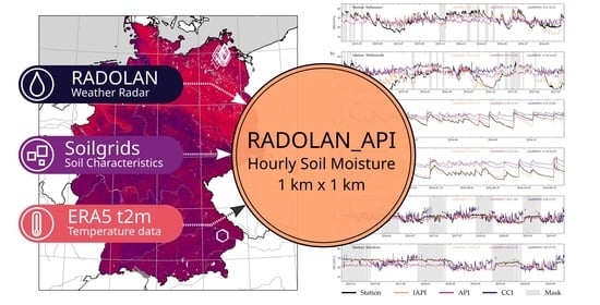
RADOLAN_API: An Hourly Soil Moisture Data Set Based on Weather Radar, Soil Properties and Reanalysis Temperature Data

Abstract

Soil moisture is a key variable in the terrestrial water and energy system. This study presents an hourly index that provides soil moisture estimates on a high spatial and temporal resolution (1 km × 1 km). The long established Antecedent Precipitation Index (API) is extended with soil characteristic and temperature dependent loss functions. The Soilgrids and ERA5 data sets are used to provide the controlling variables. Precipitation as main driver is provided by the German weather radar data set RADOLAN. Empiric variables in the equations are fitted in a optimization effort using 23 in-situ soil moisture measurement stations from the Terrestial Environmental Observatories (TERENO) and a separately conducted field campaign. The volumetric soil moisture estimation results show error values of 3.45 Vol% mean $ubRMSD$ between RADOLAN_API and station data with a high temporal accordance especially of soil moisture upsurge. Further potential of the improved API algorithm is shown with a per-station calibration of applied empirical variables. In addition, the RADOLAN_API data set was spatially compared to the ESA CCI soil moisture product where it altogether demonstrates good agreement. The resulting data set is provided as open access data.

1. Introduction

Soil moisture plays a key role in the interaction of different land surface processes and energy fluxes [1,2,3]. It controls processes like evaporation, infiltration and runoff, hence the fundamentals of the hydrological cycle [4,5]. Therefore, soil moisture influences hazards of different sorts, e.g., the extent or magnitude of floods [6]. But also temperature or precipitation extremes relate to soil moisture state and memory [7]. Soil moisture further is the main governing resource in relation to ecosystem function and form as it provides water for nutrient uptake and transpiration [8]. With that, net biome productivity and hence CO₂ fluxes are strongly linked to soil moisture variability [9]. Consequently, soil moisture has been classified as an essential climate variable (ECV) by the World Meteorological Organization’s Global Climate Observing System (WMO, GCOS) [10].

Today, measurement techniques for soil moisture are available across scales. Divers approaches allow measurement of soil moisture on point scale, e.g., gravimetric measurements, Time Domain Reflectometry (TDR) and Frequency Domain Reflectometry (FDR) but also using the attenuation of the Global Positioning System’s (GPS) signal [11,12]. Ground penetrating radar [13,14] or cosmic-ray neutron measurements, that cover bigger footprints, may also be used in mobile sampling applications and hence bridge the gap to field scale measurements of the available subsurface soil water storage [11]. Sparse station measurements combined with modeling allows for regional scale soil moisture estimations [15]. In a great effort, the International Soil Moisture Network (ISMN) collects, harmonizes and provides such sparse soil moisture measurements consisting of data streams from a multitude of individually operating networks [16].

Besides these on-site measurements, remote sensing offers retrieval opportunities for large scale spatially distributed soil moisture estimates. Imagery ranges in spatial coverage and resolution from regional UAV based sensing [17] to satellite based global soil moisture products at one single acquisition date [18,19]. Various constellations including thermal infrared, optical and microwave satellite sensor systems can be utilized to retrieve soil moisture [20,21,22,23]. Optical and thermal remote sensing allows for soil moisture estimations via the thermal-optical triangle method (TOTRAM), that interpretes the combination of pixel-based values of land surface temperature and a vegetation index, or the optical trapezoid model (OPTRAM), that utilizes the physical relationship of shortwave infrared transformed reflectance and soil moisture instead [21]. However, given the limitations regarding cloud cover a continuous stream of satellite sensed soil moisture is only possible with active and passive microwave sensors like the Advanced Scatterometer (ASCAT) [24] or the Soil Moisture Active Passive (SMAP) Mission [25,26]. Various algorithms for these platforms have been developed [18,27,28,29,30,31,32]. The spatial resolution of such data sets and retrieval algorithms usually is rather coarse with tens of kilometers [26]. Several years after the launch of the Sentinel-1 satellites, operationally provided data sets utilize the high resolution active microwave data and soil moisture data sets with higher spatial resolution of up to 1 km × 1 km are available [33,34]. The temporal resolution however depends on the revisit time of the satellites which allows for daily or half-daily data points only [26]. Yet, soil moisture data at very high resolution is sought after by different scientific communities [26]. Sub-daily data is needed to account for the highly volatile nature of soil moisture [35]. So far mostly point measurements can provide this level of temporal resolution. An hourly, continuously available spatial data set at high resolution is lacking.

In comparison, spatially distributed measurements of precipitation are available in high temporal resolution. Precipitation is the main driver for soil moisture changes in the majority of biomes [36]. There is a multitude of different precipitation measurement options [37]. Ground-based estimates range from the long established procedure of direct point measurements using rain gauges to more sophisticated methods like weather radar estimates which also deliver spatially distributed precipitation amounts [38,39]. From that, gridded precipitation products based on gauge measurements alone are developed to deliver spatial coverage [40], e.g., the global land-surface precipitation products of the Global Precipitation Climatology Centre (GPCC) [41,42]. Furthermore, mostly on national scale, ground-based weather radar precipitation data is further improved via coupling with point measurements in the effort to derive an improved, gauge-adjusted version of the spatial precipitation data set [43,44,45,46]. For several decades also satellite systems have been used for atmospheric observations [37]. Geostationary satellites carrying visible/IR sensors and low earth orbit platforms that utilize active and passive microwave imaging systems are in use [37,47]. These data sets mostly comprise a whole constellation of satellites, e.g., NASA’s Global Precipitation Measurement Mission (GPM) [48] or the PERSIANN-Climate Data Record (CDR) program which aggregates different satellite data streams and the Global Precipitation Climatology Project (GPCP) using artificial neural networks [49,50]. Reanalysis data sets like the fifth generation reanalysis data set by the European Center for Medium Range Weather Forecast (ECMWF, ERA5) [51] and sophisticated merging schemes like the Multi-Source Weighted-Ensemble Precipitation (MSWEP) [52] strive to further improve quality of gridded precipitation data sets. Still, there are flaws and weaknesses in all estimation and aggregation methods. Direct measurements of rainfall are error-prone concerning wind effects [53] and most regions lack or lose a sufficient amount of rain gauges [54]. Sun et al. [37] also demonstrate big differences and hence uncertainty in satellite and reanalysis data sets.

Still, precipitation values from such data sets correlate with change in soil moisture [55]. Considering the need for sub-daily soil moisture estimates at relatively high spatial and temporal resolution, this study introduces a precipitation based soil moisture data set. For that, we employ the German gauge-adjusted weather radar system RADOLAN [44] to derive a modified version of the Antecedent Precipitation Index (API) that directly can be used as soil moisture data set. This allows exploitation of the high sampling rate of the weather radar and also provides spatial distributed, quality controlled precipitation estimates.

Kohler and Linsley [56] introduced the concept of the API to link runoff to antecedent soil moisture conditions, which since then has been applied in varying form in several studies: research on natural hazards consults the API for different applications, e.g., in linking antecedent moisture conditions to bush fires in Australia [57] or investigating the effect of antecedent precipitation on landslides [58]. The API is still used to supplement rainfall-runoff transformation modeling [59,60,61], and subsequently it is used to support flash flood warning at ungauged locations using radar precipitation data in France [62] and Morocco [63]. But the API is not only utilized to estimate surface discharge but also to help with soil moisture assessments via exploiting the relationship to precipitation. Crow et al. [64] and Crow [65] show that errors in precipitation estimates can be evaluated with the API and also that soil moisture retrievals can be improved using the dependence of the two variables. Zhao et al. [66] discuss supplementing relative soil moisture estimates with the API. Recent studies suggest using the API directly or in conjunction with geostatistical methods to derive soil moisture estimates [67,68,69]. The API algorithm used in this study expands upon the work of Pellarin et al. [70] who in recent studies used the API in an assimilation scheme to provide a near-realtime precipitation product [71]. The proposed improved API algorithm additionally incorporates temperature data and information on soil texture composition to allow for individual dry-down rates at distinct locations. Together with higher temporal and spatial resolution precipitation input data the authors aspire to better match local traits of the course of soil moisture in terms of dry-down rates and volatility after rainfall events. The API is calculated in a temperate region in this study, as compared to previous investigations that mostly apply the idea in more arid environments [68,70]. This increases the complexity since modeling the seasonality of soil moisture does not allow for a full dry-down of the soil column in a dry season like it has been demonstrated in these other studies.

In this article we answer the question if this improved empirical soil moisture index based on the antecedent precipitation index (RADOLAN_API) is capable to resemble the course of local soil moisture measurements throughout Germany. The detection of timely upsurge of soil moisture and dry-down rates as well as depicting the seasonality with for the temperate region typical summerly depletion is of high interest in this regard. Specifically, we investigate if the proposed hourly soil moisture product matches local measurements within defined but disputed error margins of 4 Vol% soil moisture [10,72]. Furthermore, we test a version of the developed RADOLAN_API data set with local fitted empirical variables against the soil moisture station data using the same threshold of 4 Vol% defined by GCOS.

The characteristics and capabilities of the RADOLAN_API are assessed statistically on different time scales by evaluation against in-situ measurements and spatial comparisons against the ESA CCI soil moisture product. We calculate performance and error metrics in terms of correlation, bias and differences between RADOLAN_API time series and station data. Moreover, we compare the API with the satellite product on a pixel-by-pixel basis and lay out our findings in the upcoming sections. This article also serves as file descriptor for the RADOLAN_API data set, which is openly available [73]. Appendix A 

Table A1. RADOLAN_API data set description.

Filename	RADOLAN_API_v1.0.0.nc
Filetype	NetCDF4
Version	1.0.0
License	CC-BY-SA
URL	https://doi.org/10.5281/zenodo.4588904 (accessed on 27 April 2021)
File Size	20.9 GB
Dimensions	692 × 1188 × 43,824 (latitude, longitude, time)
Spatial Resolution	1 km × 1 km
Spatial Coverage	Territory of Germany
Temporal Coverage	01.01.2015–31.12.2019

provides a summary table on the file characteristics.

2. Materials and Methods

2.1. Data Sets

2.1.1. Precipitation Data Set

Precipitation data forms the fundamental base for the calculation of the proposed soil moisture data set and heavily impacts the final product. Therefore, this study uses quality controlled weather radar data of the German Weather Service (DWD, Deutscher Wetter Dienst) for the years 2015 to 2019. Specifically, the publicly available RADOLAN RW (Radar Online Adjustment) product is consulted, to meet the requirements of high spatial, temporal and radiometric resolution [74,75].

This weather radar data set holds precipitation estimates that are adjusted with gauge measurements [74]. The quality controlled precipitation sums are available at temporal, spatial, and intensity resolution of 1 h, 1 km, and 0.1 mm [44]. With that, RADOLAN delivers input and reference data for high-resolution hydrological modeling [76], rain type modeling [77], estimation of spatio-temporal variability of soil erosion [78] and (flash) flood modeling [79,80] as well as ground truth data for machine learning applications [81]. The polar-stereographic composite grid with the center point at 9.0${}^{°}$E 51.0${}^{°}$N covers the whole state territory of Germany [75,82].

All of the included C-Band weather radar stations operate on scanning intervals of 5 min and an approximate coverage of each device of a radius of 150 km. Significant overlap within the dense network ensures accurate retrievals by minimizing problems due to dampening in the signal that occur with increased distance from each sensor [83]. Furthermore, within the automatic calibration procedure, rain intensity-adapted Z-R relationships (empirical formula to estimate rainfall rates from radar reflectivity signal strength) are applied. The correction for radar artifacts contains filtering for statistical clutter and consideration of orographic shadowing effects [74,75].

Nevertheless, for a realistic estimation of the quantity of precipitation, measurements of approximately 1300 conventional stations are used for the operational hourly gauge adjustment routine [84]. These sensors basically work according to “Hellmann” ombrometers [85], which obey the standards of the World Meteorological Organization [86]. The appliance of a weighing principle and surrounding temperature-dependent heating sets the utilized devices apart from conventional measurement systems and allows capturing solid and fluid precipitation alike [75].

To derive precipitation from radar backscatter values assumptions on the drop size distribution and droplet count are necessary [83]. RADOLAN uses an extended Z-R relationship, that considers the absolute reflectivity and horizontal gradients to distinguish between typical convective and stratiform droplet distributions [75]. In wintertime, the effects of overshooting due to lower cloud heights become more prominent in weather radar systems. These shortcomings are accounted for with a seasonally-dependent correction via a regression analysis. In order to mitigate erroneous adaptation at single extreme precipitation events, e.g., intensive convective cells that occur regularly throughout Germany in summer, DWD applies a multiple polynomial regression to generate the correction factors for every pixel. Respective scanning height class, day of year, and reflectivity are therefore taken into account [83]. The weather radar data shows good agreement with NASA’s Integrated Multi-satellitE Retrievals for the Global Precipitation Measurement Mission (IMERG, GPM) satellite precipitation data set for the vegetation period [39]. This makes the data set a very good candidate as input data for the calculation of the soil moisture index with a high potential of transferability. Throughout this study, the data set will be referred to as “RADOLAN”.

2.1.2. Soil Properties

Data from the Soilgrids project [87], released by the International Soil Reference and Information Center (ISRIC), provides the information on soil properties in this study. Local clay and sand content are utilized to shape the dry-down rates of the modeled soil moisture at any given pixel. Soilgrids is a global complete soil information data set with 250 m spatial resolution and 6 layers. Based on machine learning driven algorithms that account for environmental co-variables and soil profile data, the Soilgrids data set predicts soil type and a multitude of physical and bio-chemical soil properties, e.g., distribution of soil compartments, bulk density, pH [87,88]. Soilgrid data is adapted widely by the scientific community, e.g., for generating European and global soil hydraulic databases [89,90,91] and as auxiliary variables in downscaling algorithms [91].

2.1.3. Temperature Data Set

This study uses the ERA5 single level air temperature data set (t2m) generated by the ECMWF published by the Copernicus Climate Change Service Climate Data Store (CDS) [51,92]. The ERA5 atmospheric reanalysis data set provides climate variables at hourly resolution on global scale currently covering the period from 1979 to present and as preliminary back extension from 1950 onward. Therefore, observation data is combined with model data by the technique of data assimilation in a consistent manner respecting the laws of physics [92]. For the provision at CDS the ERA5 data is interpolated to a regular 0.25${}^{°}$× 0.25${}^{°}$ grid, which for this study was further bilinearly interpolated to the RADOLAN grid. Albergel et al. [93] show that using ERA5 data as atmospheric forcing in land surface model simulations significantly improves the representation of land surface variables when compared to the predecessor ERA-Interim. Furthermore, other studies find a systematically reduced bias in ERA5 temperature and precipitation data when compared to the previous version [94,95] and indicate the high usability of the reanalysis data set in high-accuracy and high-resolution modeling scenarios [96,97].

2.1.4. Calibration and Validation Data Sets

Different data sets are used to calibrate and validate the RADOLAN_API data set. Soil moisture data from TERENO networks and a self-conducted field campaign at the Wallerfing test site is used for calibration of the necessary variables in the API equation and for validation on point data. The ISMN database provides data from the TERENO Eiffel/Lower Rhine Valley (TERENO-Rur) site [11,16,98,99]. To increase the number and diversity of in-situ measurement stations in terms of soil composition, stations from the TERENO Northeast German Lowland Observatory (TERENO-NE) site are incorporated in this study [100]. Furthermore, the self conducted field campaign holds data for six measurement stations on agricultural fields throughout the growing period of 2017. The data at each site (A2, A4, A6, P2, P4, P6) represents the respective average of five Echo EC-5 probes in 5cm depth that was corrected for diurnal cycle fluctuations.

So, for calibration and validation a total of 23 measurement stations are used. Figure 1 shows (a) the individual soil composition information derived from Soilgrids data and (b) the location of the test sites.

Table 1. Overview of soil moisture measurement stations that are used in calibration and validation procedure. Cal/Val set states the assignment to the respective random calibration and validation set.

Station	Network	Cal/Val	Coordinates	Sand	Clay	Available
		Set		[%]	[%]	Time Period
Beestland	TERENO-NE	I	53.9255${}^{°}$N, 12.9180${}^{°}$E	60	10	20111107–20191010
Boeken	TERENO-NE	II	53.9971${}^{°}$N, 13.3124${}^{°}$E	58	15	20111107–20190523
Goermin	TERENO-NE	I	53.9828${}^{°}$N, 13.2579${}^{°}$E	54	15	20111107–20191010
Grosszastrow	TERENO-NE	II	54.0170${}^{°}$N, 13.2733${}^{°}$E	59	14	20111107–20191106
Heydenhof	TERENO-NE	II	53.8682${}^{°}$N, 13.2686${}^{°}$E	52	17	20130206–20191106
Neu Tellin	TERENO-NE	I	53.8598${}^{°}$N, 13.2121${}^{°}$E	61	13	20111107–20191010
Rustow	TERENO-NE	II	53.9581${}^{°}$N, 13.0786${}^{°}$E	60	13	20111107–20191106
Sanzkow	TERENO-NE	II	53.8810${}^{°}$N, 13.1243${}^{°}$E	65	10	20111107–20191106
Sommersdorf	TERENO-NE	II	53.7899${}^{°}$N, 12.9021${}^{°}$E	58	12	20151020–20191010
Toitz	TERENO-NE	II	53.9725${}^{°}$N, 12.9906${}^{°}$E	59	14	20111107–20190910
Voelschow	TERENO-NE	I	53.8712${}^{°}$N, 13.3459${}^{°}$E	59	14	20130128–20190619
Zarrenthin	TERENO-NE	I	53.9425${}^{°}$N, 13.2857${}^{°}$E	59	13	20111107–20191107
Gevenich	TERENO-Rur	II	50.9892${}^{°}$N, 6.32355${}^{°}$E	22	16	20110804–20190403
Merzenhausen	TERENO-Rur	II	50.9303${}^{°}$N, 6.29747${}^{°}$E	21	16	20111103–20190103
Schoeneseiffen	TERENO-Rur	I	50.5149${}^{°}$N, 6.37559${}^{°}$E	28	22	20100222–20190425
Selhausen	TERENO-Rur	II	50.8691${}^{°}$N, 6.44954${}^{°}$E	19	19	20130424–20161029
Wildenrath	TERENO-Rur	II	51.1327${}^{°}$N, 6.16918${}^{°}$E	75	8	20120416–20181004
Wallerfing_A2	Wallerfing	I	48.6953${}^{°}$N, 12.8673${}^{°}$E	22	25	20160422–20161026
Wallerfing_A4	Wallerfing	I	48.6969${}^{°}$N, 12.8673${}^{°}$E	22	25	20160422–20161026
Wallerfing_A6	Wallerfing	I	48.6891${}^{°}$N, 12.8722${}^{°}$E	26	23	20160422–20161026
Wallerfing_P2	Wallerfing	I	48.6907${}^{°}$N, 12.8746${}^{°}$E	26	23	20160422–20161026
Wallerfing_P4	Wallerfing	II	48.7028${}^{°}$N, 12.8966${}^{°}$E	29	21	20160422–20161026
Wallerfing_P6	Wallerfing	I	48.7037${}^{°}$N, 12.8989${}^{°}$E	29	21	20160422–20161026

gives information on the station’s setup and their assignment to calibration and validation classes. The stations represent the typical portfolio of soil compartment distribution of Germany.

For spatial evaluation of the RADOLAN_API data set the study uses the European Space Agency’s Climate Change Initiative (ESA CCI SM) combined data set in version 4.7 [101,102,103]. The combined data set is derived through a multi-sensor merging approach that uses both active and passive publicly available Level 2 satellite products [102]. The authors chose this data set as evaluation reference because of its wide usage in the scientific community. That makes it well-established and strengths and weaknesses are well-known [104,105,106,107,108,109]. The ESA CCI SM data set is bilinearly interpolated to the RADOLAN grid for interoperability and comparability.

2.2. Antecedent Precipitation Index

The basic idea of the antecedent precipitation index (API) is to take a certain number of preceding time steps and include the respective rainfall amount in the current time step with a time dependent diminishing factor. Equation (1) shows the basic idea of the API formulated by Kohler and Linsley [56], with $API$ being the index value at time step t and $t-1$ respectively, $\gamma$ being the diminishing factor and $P_t$ representing the precipitation amount at the current time step t.

$$AP{I}_t=\gamma \times AP{I}_{t-1}+P_t$$

(1)

Derivations of this formula exist in manifold ways that allow using the API as soil moisture proxy. Crow et al. [64] e.g., apply a simple cosine based loss function that controls the summerly depletion overhead as replacement for $\gamma$. However, several single processes contribute to the reduction of soil water content represented by this diminishing factor. In this study, the antecedent precipitation index algorithm proposed by Pellarin et al. [70] is extended with additional dampening factors in the attempt to improve the empirical representation of local dominant processes that control the soil moisture loss. Temperature values from the ERA5 reanalysis data set [51,92] is used as proxy information for the upwards water loss in the soil column through evapotranspiration (Equation (3)). With that, sub-daily variations in water loss can be attributed instead of e.g., applying seasonal varying loss factors. Including this extra amount of data might be considered as immoderate contribution to a simple soil moisture index. However, this procedure will provide a better guidance in temporal scales of multiple days or weeks and hence allows e.g., for hot dry spells in summer or earlier onset of winter to be better accounted for. Local saturation state and soil properties control the amount of gravity driven drainage of soil moisture to the lower soil compartments through the process of percolation (Equation (4)). Together, factors a and b reduce the amount of soil water from time step $t-1$ to yield the current state soil moisture index $API$ at time step t:

$$AP{I}_t=a\times b\times AP{I}_{t-1}+({\theta }_{sat}-AP{I}_{t-1})\times \left[1-e^{-\frac{P_t}{d}}\right]$$

(2)

with

$$a=1-\left[\frac{T}{\alpha }\times e^{-\beta \times clay}\right]$$

(3)

and

$$b=e^{-{\left(\frac{AP{I}_{t-1}-{\theta }_{res}}{{\theta }_{sat}-{\theta }_{res}}\right)}^{\gamma }}$$

(4)

where ${\theta }_{sat}$ = maximum saturation, ${\theta }_{res}$ = residual saturation, $P_t$ = precipitation [mm], d = depth [mm], T = temperature, $\alpha$ = temperature scaling factor, $clay$ = clay content [%], $\beta$ = clay scaling factor and $\gamma \ge 1$ regulating the peak outflow. Figure 2 shows a graphical representation of the loss scaling factors a and b for different overall settings. For this study $\beta$ is fixed to 0.05 due to computational restrictions.

The saturation state in Equation (4) calculates from maximum saturation ${\theta }_{sat}$ and residual saturation ${\theta }_{res}$. The respective values are specifically derived based on empirical relationships of the Interaction Soil Biosphere Atmosphere (ISBA) model [110,111] with

$${\theta }_{sat}=0.1\times (-1.08\times \left(sand\right)+494.31)$$

(5)

$${\theta }_{res}=0.3\times {\theta }_{sat}$$

(6)

incorporating local $sand$ content. Information on soil texture composition is derived from the Soilgrids [87] data sets. The intent behind factor a is to allow quick outflow if the soil is near saturation. Loss factor b is responsible for loss due to temperature but takes clay content and an empirical scaling factor into account. In this study, we differentiate between the API, which uses empirical scaling factors optimized for all station data, and the local API (lAPI) that uses per-station optimized empirical scaling factors $\alpha$ and $\gamma$. Both indices take the respective local soil characteristics and temperature data into account.

2.3. Calibration and Validation Procedure

The coupling of precipitation information from the RADOLAN weather radar with distributed soil information and temperature data makes the retrieval of spatio-temporal API values possible. The empirical approach of the calculation implies that the variables $\alpha$ and $\gamma$ contributing to the loss factors a and b need to be adjusted for best results. Due to the lack of a valid spatially distributed ground-truth data set and computational limits the respective parameters are set constant throughout space and time for the three dimensional API calculation, which is the data represented in the RADOLAN_API data set. However, to highlight the general capacities of the advanced API algorithm itself, a local optimization of the empirical parameters (lAPI) for the single calibration sites is conducted as well. These lAPI realisations on point scale also include local temperature and soil information data but furthermore individually adjusted $\alpha$ and $\gamma$ values (

Table A2. Values of variables $\alpha$ and $\gamma$ for overall and individual (local) optimization and variable values in the respective cross validation class (rounded).

	Overall Opt.		Local Opt.		CV Class I Calibration		CV Class II Calibration
Station	$\mathit{\alpha }$	$\mathit{\gamma }$	$\mathit{\alpha }$	$\mathit{\gamma }$	$\mathit{\alpha }$	$\mathit{\gamma }$	$\mathit{\alpha }$	$\mathit{\gamma }$
Beestland	19,768.0102	6.9960	25,888.4543	6.7393	-	-	23,704.3638	7.0166
Boeken	19,768.0102	6.9960	15,459.5184	8.6683	-	-	23,704.3638	7.0166
Goermin	19,768.0102	6.9960	13,407.3887	8.9687	-	-	23,704.3638	7.0166
Grosszastrow	19,768.0102	6.9960	13,103.0731	8.7054	16,265.6752	7.0217	-	-
Heydenhof	19,768.0102	6.9960	13,002.0141	10.3239	-	-	23,704.3638	7.0166
Neu Tellin	19,768.0102	6.9960	17,048.6849	7.9655	16,265.6752	7.0217	-	-
Rustow	19,768.0102	6.9960	18,155.6516	8.7882	16,265.6752	7.0217	-	-
Sanzkow	19,768.0102	6.9960	15,280.2734	12.2186	-	-	23,704.3638	7.0166
Sommersdorf	19,768.0102	6.9960	15,931.4899	7.4929	16,265.6752	7.0217	-	-
Toitz	19,768.0102	6.9960	26,363.4512	8.3422	-	-	23,704.3638	7.0166
Zarrenthin	19,768.0102	6.9960	24,362.5183	6.5954	-	-	23,704.3638	7.0166
Gevenich	19,768.0102	6.9960	3238.0722	11.7320	16,265.6752	7.0217	-	-
Merzenhausen	19,768.0102	6.9960	3399.5669	14.6008	16,265.6752	7.0217	-	-
Schoeneseiffen	19,768.0102	6.9960	4502.4258	36.9911	16,265.6752	7.0217	-	-
Selhausen	19,768.0102	6.9960	4390.2302	15.1374	16,265.6752	7.0217	-	-
Wildenrath	19,768.0102	6.9960	4129.9100	13.6303	-	-	23,704.3638	7.0166
Wallerfing_A2	19,768.0102	6.9960	2991.0367	7.0635	16,265.6752	7.0217	-	-
Wallerfing_A4	19,768.0102	6.9960	4604.2422	6.2033	16,265.6752	7.0217	-	-
Wallerfing_A6	19,768.0102	6.9960	3552.1796	4.0507	-	-	23,704.3638	7.0166
Wallerfing_P2	19,768.0102	6.9960	3009.0580	5.6143	16,265.6752	7.0217	-	-
Wallerfing_P6	19,768.0102	6.9960	3115.7178	3.3863	-	-	23,704.3638	7.0166
Wallerfing_P4	19,768.0102	6.9960	3612.4949	5.8123	-	-	23,704.3638	7.0166

).

Three main measures are used for the evaluation of the proposed data set: bias, unbiased root mean square difference ($ubRMSD$) and Pearson’s R linear correlation coefficient.

$$bias=\frac{1}{N}\sum _{i=1}^N(x_i-y_i)$$

(7)

$$\mathrm{RMSD}=\sqrt{\frac{1}{N}\sum _{i=1}^N{(x_i-y_i)}^2}$$

(8)

$$\mathrm{ubRMSD}=\sqrt{RMS{D}^2-bia{s}^2}$$

(9)

$$R=\frac{{\sigma }_{xy}}{{\sigma }_x{\sigma }_y}$$

(10)

Quality flags of ISMN and TERENO data sets are respected for calibration and cross-validation. ESA CCI SM data also ships with quality flags. Such, that indicate snow or cold temperatures are used for all data sets in the point scale evaluation (API, station measurement data and ESA CCI SM data) and also for the spatial evaluation of the RADOLAN_API against ESA CCI SM data. Therefore, a seven day rolling window is additionally applied to help with excluding days after or in between freezing. Remaining quality flags concerning the data quality of ESA CCI SM data itself are only applied to the satellite data set.

Soil moisture data of the TERENO network and the conducted field campaign is used to calibrate the empirical parameters of the API formula that determine the effect of loss factors a and b in Equation (2). The respective stations only provide data for a specific time span and hence calibration was done for the particular available period while omitting a 14 day warm-up period.

Calibration of the respective empirical variables of the API demanded for iteratively calculating the described hourly soil moisture index for each of the 23 single reference stations. Depths of measurement and local soil composition of each installation therefore is taken into account. The applied optimization procedure evaluates the calculations against measured soil moisture station data. In case of the API (RADOLAN_API) version, the minimization target is defined as the mean $RMSD$ across all stations against the measured data. The empirical variables $\alpha$ and $\gamma$ are optimized iteratively and finally selected based on the outcome of the procedure. For the individually optimized lAPI on point scale, the variables are optimized on a per-station basis. In both variants, the whole available time series was used at each point with no masking besides respecting the warm-up period. The Nelder-Mead algorithm is used for minimization of the respective target variable (mean) $RMSE$ [112]. Gao and Han [113] state that this is the most widely applied direct search method for unconstrained optimization problems and further improved the algorithm for solving problems more efficiently in high dimensions.

For validation purposes the soil moisture stations are randomly split and assigned to two sets, I and II (Table 1), to carry out a standard cross-validation. Hence, the calibration approach described above is repeated for the respective calibration subset of stations and the resulting empirical variables are used to validate the remaining subset against the appropriate soil moisture station data. Table A2 gives an overview of respective $\alpha$ and $\gamma$ values for the overall and local individual optimization as well as the calibration sets.

This study also evaluates the API spatially against ESA CCI data on a pixel-by-pixel basis. Additional to the overall comparison, a monthly and seasonal summary is conducted to provide insights in the temporal dependence of the performance. Furthermore, the local calibrated lAPI time series at the measurement sites are compared to the measurements. The results aim to show the adaptability of the API to local circumstances.

3. Results

3.1. Calibration and Evaluation

The calibration for RADOLAN_API resulted in a mean $ubRMSD$ of 3.37 Vol% with a standard deviation of 1.93 Vol% between the calculated API on point scale and respective reference measurements. Table 3 summarizes the evaluation metrics. The spatial distributed API data set RADOLAN_API is published as CC-BY-SA in form of a netCDF file [73]. The hourly resolution and 1 km × 1 km spatial resolution add up to a data set with dimensions 692 × 1188 × 43,824 (latitude, longitude, time) and a file size of 20.9 GBs that covers the years 2015 to 2019. A summary of the file characteristics is presented in Table A1. In the following “API” refers to the variant of the index included in this soil moisture data set.

The evaluation of the proposed API against ESA CCI SM data and station data respects masking based on the ESA CCI SM flags as described in Section 2.3. Hence, values of metrics in the evaluation differ to the ones obtained in the calibration process itself. This is done to allow the calibration of the empiric variables to also account for seasonality in terms of rising soil moisture in fall and higher soil moisture values after winter. However, for a fair comparison and comparability, the flagged time spans, highlighted in grey in Figure 3, are excluded for the remaining evaluation. That figure shows the best and worst performing station of each network relating to $RMSD$ between API and measurement. Further insight in the exact metrics is given in

Table 2. Evaluation of the overall and locally optimized API and ESA CCI SM data against local measurements; and evaluation of ESA CCI SM against overall optimized API; masks are applied as described in the text; the asterisk (*) indicate lower ($ub$)$RMSD$ and higher R values of the API respectively in comparison to ESA CCI SM data when benchmarked against the local measurements.

	RMSD [Vol%]				ubRMSD [Vol%]				R
	In-Situ			CCI	In-Situ			CCI	In-Situ			CCI
Station	API	lAPI	CCI	API	API	lAPI	CCI	API	API	lAPI	CCI	API
Beestland	2.29 *	2.02 *	5.19	5.77	2.16 *	2.02 *	3.26	3.27	0.69 *	0.69 *	0.56	0.55
Boeken	2.19 *	1.76 *	4.34	4.58	1.88 *	1.76 *	4.32	4.36	0.60 *	0.71 *	0.42	0.40
Goermin	2.83 *	2.29 *	4.34	4.41	2.78 *	2.29 *	4.30	4.30	0.64 *	0.77 *	0.50	0.44
Grosszastrow	3.09 *	2.67 *	5.19	4.76	3.09 *	2.67 *	4.87	4.51	0.60 *	0.71 *	0.36	0.28
Heydenhof	2.93 *	2.03 *	4.49	4.28	2.15 *	2.02 *	4.01	4.28	0.67 *	0.71 *	0.53	0.44
Neu Tellin	1.84 *	1.72 *	4.26	4.62	1.84 *	1.71 *	3.37	3.80	0.77 *	0.80 *	0.59	0.41
Rustow	2.67 *	2.29 *	3.79	3.99	2.30 *	2.28 *	3.78	3.69	0.59 *	0.63 *	0.48	0.49
Sanzkow	4.04	2.28 *	3.87	4.12	2.72 *	2.28 *	3.77	3.51	0.70 *	0.79 *	0.55	0.59
Sommersdorf	2.01 *	1.81 *	4.21	4.32	2.00 *	1.81 *	2.82	3.25	0.76 *	0.80 *	0.71	0.60
Toitz	2.59 *	1.55 *	3.07	3.91	1.55 *	1.55 *	3.06	3.25	0.72 *	0.71 *	0.63	0.57
Voelschow	3.21*	1.74 *	4.27	4.48	2.03*	1.73*	4.07	4.34	0.61 *	0.76 *	0.52	0.43
Zarrenthin	2.96 *	2.87 *	4.72	4.24	2.91*	2.83*	4.56	4.21	0.32	0.32	0.33	0.41
Gevenich	7.94 *	4.51 *	8.84	3.74	7.35	4.51 *	6.67	2.61	0.62	0.84 *	0.69	0.59
Merzenhausen	8.09	6.51 *	7.12	4.30	7.84	6.50	5.76	3.84	0.05	0.57	0.68	0.21
Schoeneseiffen	8.90	3.87 *	6.99	4.30	7.20	3.87 *	6.80	2.52	0.54	0.88 *	0.59	0.47
Selhausen	5.91	4.15 *	4.21	3.56	5.62	4.15 *	4.21	3.04	0.51	0.77	0.81	0.42
Wildenrath	8.87 *	5.01 *	11.54	4.80	6.96	5.00 *	6.42	2.60	0.44	0.77 *	0.57	0.54
Wallerfing_A2	4.29 *	3.14 *	6.33	3.46	3.31	3.12	2.92	1.98	0.51	0.65	0.70	0.47
Wallerfing_A4	4.89 *	4.01 *	6.64	3.46	4.00	3.99	3.38	1.98	0.40	0.45	0.68	0.47
Wallerfing_A6	7.52 *	2.75 *	9.24	2.46	2.73 *	2.70 *	2.76	1.68	0.76 *	0.73	0.75	0.65
Wallerfing_P2	5.19 *	2.75 *	6.85	2.50	2.76 *	2.68 *	2.77	1.67	0.76 *	0.74	0.75	0.65
Wallerfing_P4	4.30 *	1.80 *	7.12	3.32	2.15 *	1.80 *	2.54	1.56	0.81 *	0.86 *	0.72	0.65
Wallerfing_P6	8.72 *	2.03 *	11.26	2.92	2.10 *	2.03 *	2.63	1.57	0.81 *	0.81 *	0.63	0.65
Mean	4.66 *	2.85 *	5.99	4.01	3.45 *	2.84 *	4.05	3.12	0.60	0.72 *	0.60	0.49
Standard dev.	2.47	1.27 *	2.36	0.77	2.01	1.27 *	1.30	1.02	0.18	0.13	0.13	0.12

where also metrics for ESA CCI SM versus measurements and ESA CCI SM versus API are included.

The overall optimized API shows a mean $RMSD$ of 4.66 Vol% and $ubRMSD$ of 3.45 Vol% with a respective standard deviation across the 23 point results of 2.47 Vol% and 2.01 Vol% when compared to in-situ station measurements. With that, the differences to measurement data are smaller than for the ESA CCI SM data set in the same comparison (5.99 Vol% and 4.05 Vol% respectively). However, the API shows wider spread and deviation in both $RMSD$ and $ubRMSD$. The API data set reaches the highest mismatch in $RMSD$ and $ubRMSD$ to the station Wildenrath with 8.87 Vol% and 6.96 Vol% respectively. This station shows extremely low soil moisture values during summer (Figure 3b) which can be traced back to the high sand and low clay content at that site (Table 1). Lowest difference is reached at station Neu Tellin with 1.84 Vol% ($RMSD$) and for unbiased comparison station Toitz with 1.55 Vol% ($ubRMSD$). Generally, the sandier sites of the TERENO-NE site perform noticeable better than stations from the other networks.

Overall, the API is similarly correlated to the in-situ measurements like the ESA CCI SM data is, with a mean correlation coefficient of 0.60. Here again, the API shows a higher standard deviation of 0.18 compared to 0.13 of ESA CCI SM data. Expectedly, the lAPI shows increased correlation to the soil moisture measurements with a mean of 0.72 and maximum of 0.88. This higher accordance is shown clearly in Figure 3 where the lAPI distinctly follows the summerly depletion for TERENO-Rur and TERENO-NE time series. The scatterplots demonstrate the improvements accordingly. For Wallerfing sites where there is no seasonality or summerly depletion to follow, the lAPI shows higher and prolonged outflow. This results in a difference in $RMSD$ of −1.15 Vol% and −6.69 Vol% and also lowered $ubRMSD$ that is reduced by 0.16 Vol% and 0.07 Vol% for the stations Wallerfing A2 and Wallerfing P6 respectively. The temporal accuracy and dynamic of the API and lAPI do match the measurement data very well which also the Wallerfing plots (Figure 3b,c) demonstrate clearly. This is the direct effect of the high resolution of the RADOLAN product that directly propagates into a rise in soil moisture.

3.2. Two-Fold Cross-Validation

The stations are randomly assigned to two groups I and II for the cross-validation (CV) procedure. Table 1 gives the respective affiliation. Each group is used as calibration and validation group respectively. Run I of the CV uses stations of set I as calibration data and stations of set II as validation data and vice versa for run II. Overall, the cross validation shows in average very similar evaluation metrics like the overall calibration that uses all stations at once (

Table 3. Calibration results of API depletion factors and averaged evaluation metrics for overall calibration and calibration in the cross-validation scheme (no masking applied).

Run	RMSD [Vol%]	ubRMSD [Vol%]	R
Overall Calibration	mean: 4.65 stdev: 2.37	mean: 3.37 stdev: 1.93	mean: 0.61 stdev: 0.15
Avg. of Cross-Validation	mean: 4.72 stdev: 2.29	mean: 3.38 stdev: 1.93	mean: 0.61 stdev: 0.16
Run I: Validation Set	mean: 4.48 stdev: 2.13	mean: 2.59 stdev: 1.28	mean: 0.66 stdev: 0.12
Run II: Validation Set	mean: 4.99 stdev: 2.43	mean: 4.25 stdev: 2.13	mean: 0.55 stdev: 0.17

). The mean $RMSD$ only increases by 0.07 Vol% to 4.72 Vol% where the standard deviation in the combined validation data set even declines.

In run I the $RMSD$ drops whereas in run II the $RMSD$ with 4.99 Vol% is higher than in the overall calibration. The correlation coefficient behaves similar: the R of both validation sets combined does not change compared to the overall calibration, however run I validation set outperforms the run II validation set. This difference becomes more prominent for the $ubRMSD$. Both validation sets combined, the error metric does not significantly change compared to the overall calibration with 4.72 Vol% and 4.65 Vol%. But validation in the cross-validation run I outperforms run II validation with 2.59 Vol% $ubRMSD$ compared to 4.25 Vol% $ubRMSD$. Standard deviation values increase in run II validation accordingly. Figure 4 clearly presents this fact. Whereas $RMSD$ and R do not deviate much from the average distribution, the $ubRMSD$ values for run I and II distinctly differ with a wide spread (standard deviation of 2.13 Vol%) of the metric for the validation set in run II and a compact distribution of $ubRMSD$ for run I (standard deviation 1.28 Vol%). The disparity is to be attributed to the random partition of stations in the two sets: every group got a majority of a distinctive set of soil types (Table 1). Run I with stations of group II as validation stations holds many of the better performing stations, when calibrated separately, mostly of the TERENO-NE site.

3.3. Comparison with ESA CCI Soil Moisture Data

The API was compared to ESA CCI SM data on a pixel by pixel basis. Figure 5 shows the $ubRMSD$, bias and correlation coefficient R for three seasons MAM, JJA, SON and the mean over all three of them. It becomes apparent that in the spring season MAM the differences are highest with $ubRMSD$ values exceeding 4 Vol% in central Germany. Similar patterns are observable for seasons JJA and SON where these are not as pronounced. Outlines of the low mountain range in the central part of Germany e.g., the Harz Mountains (51.7${}^{°}$N, 10.7${}^{°}$E) or Pfälzerwald (49.3${}^{°}$N, 7.9${}^{°}$E) are reflected in the $ubRMSD$. Most prominently however, the errors are highest in the east of the Rothhaargebirge (~51.0${}^{°}$N, 9.0${}^{°}$E) which is justified with a monthly unsteady bias ranging from negative to positive values in the MAM season (Figure A1). In the northeastern part of Germany dissimilarity of the API and ESA CCI SM data is prevalent. At the TERENO sites in this region the API outperformed the ESA CCI SM product (Table 2). A clear reflection of soil types is not to be seen in the error values (Figure 1).

Overall a negative bias of the API compared to the ESA CCI SM product exists, which similarly was present in the per-station comparison. The negative bias of the API in the spatial comparison is most noticeable along river Elbe (52.5${}^{°}$N, 11.7${}^{°}$E) and in north western Germany (East Frisia, 53.5${}^{°}$N, 7.9${}^{°}$E). In the Harz Mountains the API values are positivly biased which can possibly be attributed to higher precipitation amounts due to orographic rainfall.

Correlation between the ESA CCI SM and the API data set ranges between a R value of 0.4 and 0.8 with lower values in the MAM season. Figure 6 depicts the spatially aggregated evaluation between ESA CCI SM an and API on a monthly basis. It has to be noted, that for masking reasons only about half of the amount of grid cells are available for the winter period (Figure A2). The monthly evaluation supports the statement of low correlation (with high standard deviation) and higher bias in wintertime where the overall optimized API does not deliver soil moisture values as high as ESA CCI SM does. The monthly mean $ubRMSD$ in the MAM season ranges from 1.0 to 2.0 Vol% (Figure 6 and Figure A1) which does not reflect the strong deviation from the seasons JJA and SON as shown in Figure 5 due to the discussed shift in bias.

4. Discussion

The introduced RADOLAN_API data set shows very good agreement with local soil moisture measurements in terms of volumetric soil moisture estimation with a mean $ubRMSD$ of 3.45 Vol% and mean $RMSD$ of 4.66 Vol% in the evaluation against 23 measurement stations. The unbiased error values of the hourly soil moisture data set fulfill the criteria of GCOS which proclaims an error threshold of 4 Vol% for soil moisture estimations. With that, RADOLAN_API shows lower mean $ubRMSD$ and lower mean $RMSD$ values than ESA CCI SM (4.05 Vol% and 5.99 Vol%) at the utilized soil moisture measurement stations (Table 2). An especially strong argument for the weather radar based API is the timely increase of modeled soil moisture that clearly hits the measured upsurge. This is perfectly visible in comparison to station measurements in Figure 3c,d. Delivering this high accuracy in the change signal is a very valuable characteristic and often sought after in the modeling community [26]. Consequently, on point scale, the API outperforms ESA CCI SM data at 16 of 23 stations with regard to $ubRMSD$ against measurement data. This might be explained with the higher spatial and temporal resolution in the original data set than the merged satellite product. Also vegetation influence is reasonably handled in the empiric loss functions of the proposed API.

Additionally, we introduced a locally optimized API (lAPI), that similarly considers soil information and temperature but empirical scaling variables are locally adjusted. Seasonalities of highly volatile soil moisture time series can be even better represented with the lAPI than the overall optimized API. This is convincingly presented in the exemplary station plots in Figure 3. The correlation between modeled data and measurements increases accordingly from a R value of 0.60 (API) to 0.72 (lAPI, Table 2).

The cross-validation procedure of the API shows little differences in validation results of the two respective sets. This means that on the one hand the API formula is robust. On the other hand the need for a local, more individual adjustment based e.g., on relationships between soil properties and actually applied values of the depletion variables is evident. Accordingly, Table 2 shows improvements in all averaged metrics $RMSD$, $ubRMSD$ and R for the lAPI compared to the API.

Investigation on different temporal resolutions by showing monthly and seasonal aggregates of error and correlation metrics is necessary to get unambiguous results [72]. This approach allowed the authors to identify a local non-stationary bias in the western part of Germany conducting the spatial comparison of the API and ESA CCI SM data.

A dominant pattern of negative biased API values in the southern part of Germany is prevalent. For these regions, the ESA CCI SM data set shows strikingly high mean soil moisture estimates (Figure A3). Missing sensor data in the constellation contributing to ESA CCI SM data can lead to differences in soil moisture estimates [101]. In this regard, an accumulation of acquisitions that use a specific sensor combination while featuring the distinct bias pattern, could however not be confirmed as possible reason (Figure A3). These high values in the ESA CCI SM data set coincide with occurrences of Leptosols and Cambisols from material derived from limestone, marlstone and dolomite weathering [114]. In the same region the hydrogeology is dominated by karstified or fissured jurassic calcareous fazies in the base rock [115]. The attributed low air capacity of the effective root zone and indicated low soil moisture at field capacity for this area does not fit the behaviour of the ESA CCI SM data [116,117]. Wagner [118] discusses unexpected backscatter effects in microwave satellite data. Increased surface roughness of dry soils containing rock fragments in the top layer might be the explanation for the very high soil moisture values in these regions [118].

Many processes and properties on earth’s surface that affect the water and energy fluxes are not directly included in the proposed empirical API model that seeks to avoid the input data overhead. The two most obvious of these factors might be soil organic carbon (SOC) and vegetation cover: predominantly in dry conditions, SOC explains variance better than soil texture [119]. Furthermore, de la Torre et al. [120] show that vegetation strongly influences soil dry-down rates through evapotranspiration. Empirically modeling the manifold effects that vegetation related processes have on soil moisture in the API formula certainly holds error potential. Yet, the results at the single measurement station sites indicate that the diverse interactions were well mimicked with the applied loss functions at least for grasslands and agricultural sites.

Still, uncertainties in the utilized data sets propagate and introduce errors in the soil moisture estimation. Tifafi et al. [121] e.g., point out spatial representativeness errors in the Soilgrids data set, specifically however for the modeled soil organic carbon. Also, inaccuracies in the RADOLAN data set directly propagate into the API values. Good overall agreement of the weather radar data with the renowned GPM data set has been shown but seasonal differences in performance may be the reasoning for the higher negative bias values in the eastern part of Germany [39]. An investigation of the effects of such input data inherent deficiencies has not been carried out by the authors and is not in the scope of this article. Usage of further downscaled soil texture information as shown by Marzahn and Meyer [122] can guide the way of the proposed API towards field scale soil moisture estimations.

5. Conclusions

This study introduces the hourly weather radar data, temperature and soil information based soil moisture data set RADOLAN_API. The utilized empirical variables in the API formula are once optimized to be used in the spatial API data set RADOLAN_API, but also on a per-station basis to evaluate the adjustability of the improved API algorithm to given specific circumstances concerning interplay of soil characteristics and natural surroundings. Evaluation of the modeled soil moisture data was conducted on different temporal resolutions, covering daily, monthly and seasonal aggregations.

The API generally shows good agreement with measured data especially for timely detection of the onset of soil moisture increase. This characteristic is taken from the high temporal resolution of the RADOLAN weather radar data input. Also, performance of the RADOLAN_API in terms of error metrics against in-situ soil moisture data is very good with a mean $ubRMSD$ of 3.45 Vol% across 23 stations and hence complies with the GCOS threshold of 4 Vol%. The local adjusted API accomplishes an $ubRMSD$ of 2.84 Vol% against said stations, mostly because the individual seasonality can be better depicted on different soils with local optimization of the empirical parameters in the API algorithm.

Thus, the API is capable of rendering the soil moisture development on point scale and spatially distributed with a focus on detection of rapid moisture change. It has been shown that the per-station optimized API data set greatly benefits from a local optimization of the empirical variables and allows for better representation of seasonal variability than the overall optimized API. Hence, the authors suggest to establish a relationship between soil properties and the locally adjusted empirical loss factors through e.g., cluster analysis in further research. Usage of soil texture data of even higher spatial resolution for downscaling the API needs to be discussed. Independent of eventually investigated spatial scales, a set of distributed empirical factors regulating the soil moisture dry-down would further improve the empirical modeling of soil moisture with the API, because local prevailing soil conditions could be more individually considered.

Overall, integrating weather radar data in the soil moisture estimation scheme showed to be very beneficial. A high temporal resolution soil moisture data set option for Germany is now available to the scientific community.

References

1. Legates, D.R.; Mahmood, R.; Levia, D.F.; DeLiberty, T.L.; Quiring, S.M.; Houser, C.; Nelson, F.E. Soil moisture: A central and unifying theme in physical geography. Prog. Phys. Geogr. Earth Environ. 2010, 35, 65–86. [Google Scholar] [CrossRef]
2. Miralles, D.G.; van den Berg, M.J.; Teuling, A.J.; de Jeu, R.A.M. Soil moisture-temperature coupling: A multiscale observational analysis. Geophys. Res. Lett. 2012, 39. [Google Scholar] [CrossRef] [Green Version]
3. McPherson, R.A. A review of vegetation—atmosphere interactions and their influences on mesoscale phenomena. Prog. Phys. Geogr. Earth Environ. 2007, 31, 261–285. [Google Scholar] [CrossRef]
4. Babaeian, E.; Sadeghi, M.; Franz, T.E.; Jones, S.; Tuller, M. Mapping soil moisture with the OPtical TRApezoid Model (OPTRAM) based on long-term MODIS observations. Remote Sens. Environ. 2018, 211, 425–440. [Google Scholar] [CrossRef]
5. Al-Yaari, A.; Wigneron, J.P.; Dorigo, W.; Colliander, A.; Pellarin, T.; Hahn, S.; Mialon, A.; Richaume, P.; Fernandez-Moran, R.; Fan, L.; et al. Assessment and inter-comparison of recently developed/reprocessed microwave satellite soil moisture products using ISMN ground-based measurements. Remote Sens. Environ. 2019, 224, 289–303. [Google Scholar] [CrossRef]
6. Chifflard, P.; Kranl, J.; zur Strassen, G.; Zepp, H. The significance of soil moisture in forecasting characteristics of flood events. A statistical analysis in two nested catchments. J. Hydrol. Hydromech. 2018, 66, 1–11. [Google Scholar] [CrossRef] [Green Version]
7. Hirschi, M.; Seneviratne, S.I.; Alexandrov, V.; Boberg, F.; Boroneant, C.; Christensen, O.B.; Formayer, H.; Orlowsky, B.; Stepanek, P. Observational evidence for soil-moisture impact on hot extremes in southeastern Europe. Nat. Geosci. 2010, 4, 17–21. [Google Scholar] [CrossRef]
8. Robinson, D.A.; Campbell, C.S.; Hopmans, J.W.; Hornbuckle, B.K.; Jones, S.B.; Knight, R.; Ogden, F.; Selker, J.; Wendroth, O. Soil Moisture Measurement for Ecological and Hydrological Watershed-Scale Observatories: A Review. Vadose Zone J. 2008, 7, 358–389. [Google Scholar] [CrossRef] [Green Version]
9. Green, J.K.; Seneviratne, S.I.; Berg, A.M.; Findell, K.L.; Hagemann, S.; Lawrence, D.M.; Gentine, P. Large influence of soil moisture on long-term terrestrial carbon uptake. Nature 2019, 565, 476–479. [Google Scholar] [CrossRef] [PubMed]
10. GCOS. The Global Observing System for Climate: Implementation Needs; WMO Pub GCOS-200: Geneva, Switzerland, 2016. [Google Scholar]
11. Dorigo, W.A.; Wagner, W.; Hohensinn, R.; Hahn, S.; Paulik, C.; Xaver, A.; Gruber, A.; Drusch, M.; Mecklenburg, S.; van Oevelen, P.; et al. The International Soil Moisture Network: A data hosting facility for global in situ soil moisture measurements. Hydrol. Earth Syst. Sci. 2011, 15, 1675–1698. [Google Scholar] [CrossRef] [Green Version]
12. Koch, F.; Schlenz, F.; Prasch, M.; Appel, F.; Ruf, T.; Mauser, W. Soil Moisture Retrieval Based on GPS Signal Strength Attenuation. Water 2016, 8, 276. [Google Scholar] [CrossRef]
13. Zhou, L.; Yu, D.; Wang, Z.; Wang, X. Soil Water Content Estimation Using High-Frequency Ground Penetrating Radar. Water 2019, 11, 1036. [Google Scholar] [CrossRef] [Green Version]
14. Lombardi, F.; Lualdi, M. Step-Frequency Ground Penetrating Radar for Agricultural Soil Morphology Characterisation. Remote Sens. 2019, 11, 1075. [Google Scholar] [CrossRef] [Green Version]
15. Crow, W.T.; Berg, A.A.; Cosh, M.H.; Loew, A.; Mohanty, B.P.; Panciera, R.; de Rosnay, P.; Ryu, D.; Walker, J.P. Upscaling sparse ground-based soil moisture observations for the validation of coarse-resolution satellite soil moisture products. Rev. Geophys. 2012, 50. [Google Scholar] [CrossRef] [Green Version]
16. Dorigo, W.; Xaver, A.; Vreugdenhil, M.; Gruber, A.; Hegyiová, A.; Sanchis-Dufau, A.; Zamojski, D.; Cordes, C.; Wagner, W.; Drusch, M. Global Automated Quality Control of In Situ Soil Moisture Data from the International Soil Moisture Network. Vadose Zone J. 2013, 12. [Google Scholar] [CrossRef]
17. Wu, K.; Rodriguez, G.A.; Zajc, M.; Jacquemin, E.; Clément, M.; Coster, A.D.; Lambot, S. A new drone-borne GPR for soil moisture mapping. Remote Sens. Environ. 2019, 235, 111456. [Google Scholar] [CrossRef]
18. Wagner, W. Evaluation of the agreement between the first global remotely sensed soil moisture data with model and precipitation data. J. Geophys. Res. 2003, 108. [Google Scholar] [CrossRef]
19. Wang, Y.; Leng, P.; Peng, J.; Marzahn, P.; Ludwig, R. Global assessments of two blended microwave soil moisture products CCI and SMOPS with in-situ measurements and reanalysis data. Int. J. Appl. Earth Obs. Geoinf. 2021, 94, 102234. [Google Scholar] [CrossRef]
20. Babaeian, E.; Sadeghi, M.; Jones, S.B.; Montzka, C.; Vereecken, H.; Tuller, M. Ground, Proximal, and Satellite Remote Sensing of Soil Moisture. Rev. Geophys. 2019, 57, 530–616. [Google Scholar] [CrossRef] [Green Version]
21. Sadeghi, M.; Babaeian, E.; Tuller, M.; Jones, S.B. The optical trapezoid model: A novel approach to remote sensing of soil moisture applied to Sentinel-2 and Landsat-8 observations. Remote Sens. Environ. 2017, 198, 52–68. [Google Scholar] [CrossRef] [Green Version]
22. Piles, M.; Petropoulos, G.P.; Sánchez, N.; González-Zamora, Á.; Ireland, G. Towards improved spatio-temporal resolution soil moisture retrievals from the synergy of SMOS and MSG SEVIRI spaceborne observations. Remote Sens. Environ. 2016, 180, 403–417. [Google Scholar] [CrossRef] [Green Version]
23. Ghilain, N.; Arboleda, A.; Batelaan, O.; Ardö, J.; Trigo, I.; Barrios, J.M.; Gellens-Meulenberghs, F. A New Retrieval Algorithm for Soil Moisture Index from Thermal Infrared Sensor On-Board Geostationary Satellites over Europe and Africa and Its Validation. Remote Sens. 2019, 11, 1968. [Google Scholar] [CrossRef] [Green Version]
24. Bartalis, Z.; Wagner, W.; Naeimi, V.; Hasenauer, S.; Scipal, K.; Bonekamp, H.; Figa, J.; Anderson, C. Initial soil moisture retrievals from the METOP-A Advanced Scatterometer (ASCAT). Geophys. Res. Lett. 2007, 34. [Google Scholar] [CrossRef] [Green Version]
25. Entekhabi, D.; Njoku, E.G.; O’Neill, P.E.; Kellogg, K.H.; Crow, W.T.; Edelstein, W.N.; Entin, J.K.; Goodman, S.D.; Jackson, T.J.; Johnson, J.; et al. The Soil Moisture Active Passive (SMAP) Mission. Proc. IEEE 2010, 98, 704–716. [Google Scholar] [CrossRef]
26. Peng, J.; Albergel, C.; Balenzano, A.; Brocca, L.; Cartus, O.; Cosh, M.H.; Crow, W.T.; Dabrowska-Zielinska, K.; Dadson, S.; Davidson, M.W.; et al. A roadmap for high-resolution satellite soil moisture applications – confronting product characteristics with user requirements. Remote Sens. Environ. 2021, 252, 112162. [Google Scholar] [CrossRef]
27. Merzouki, A.; McNairn, H.; Powers, J.; Friesen, M. Synthetic Aperture Radar (SAR) Compact Polarimetry for Soil Moisture Retrieval. Remote Sens. 2019, 11, 2227. [Google Scholar] [CrossRef] [Green Version]
28. Choker, M.; Baghdadi, N.; Zribi, M.; Hajj, M.E.; Paloscia, S.; Verhoest, N.; Lievens, H.; Mattia, F. Evaluation of the Oh, Dubois and IEM Backscatter Models Using a Large Dataset of SAR Data and Experimental Soil Measurements. Water 2017, 9, 38. [Google Scholar] [CrossRef]
29. Ochsner, T.E.; Cosh, M.H.; Cuenca, R.H.; Dorigo, W.A.; Draper, C.S.; Hagimoto, Y.; Kerr, Y.H.; Larson, K.M.; Njoku, E.G.; Small, E.E.; et al. State of the Art in Large-Scale Soil Moisture Monitoring. Soil Sci. Soc. Am. J. 2013, 77, 1888–1919. [Google Scholar] [CrossRef] [Green Version]
30. Kerr, Y.; Waldteufel, P.; Wigneron, J.P.; Martinuzzi, J.; Font, J.; Berger, M. Soil moisture retrieval from space: The Soil Moisture and Ocean Salinity (SMOS) mission. IEEE Trans. Geosci. Remote Sens. 2001, 39, 1729–1735. [Google Scholar] [CrossRef]
31. Naeimi, V.; Scipal, K.; Bartalis, Z.; Hasenauer, S.; Wagner, W. An Improved Soil Moisture Retrieval Algorithm for ERS and METOP Scatterometer Observations. IEEE Trans. Geosci. Remote Sens. 2009, 47, 1999–2013. [Google Scholar] [CrossRef]
32. Owe, M.; de Jeu, R.; Walker, J. A methodology for surface soil moisture and vegetation optical depth retrieval using the microwave polarization difference index. IEEE Trans. Geosci. Remote Sens. 2001, 39, 1643–1654. [Google Scholar] [CrossRef] [Green Version]
33. Das, N.N.; Entekhabi, D.; Dunbar, R.S.; Chaubell, M.J.; Colliander, A.; Yueh, S.; Jagdhuber, T.; Chen, F.; Crow, W.; O’Neill, P.E.; et al. The SMAP and Copernicus Sentinel 1A/B microwave active-passive high resolution surface soil moisture product. Remote Sens. Environ. 2019, 233, 111380. [Google Scholar] [CrossRef]
34. Bauer-Marschallinger, B.; Paulik, C.; Hochstöger, S.; Mistelbauer, T.; Modanesi, S.; Ciabatta, L.; Massari, C.; Brocca, L.; Wagner, W. Soil Moisture from Fusion of Scatterometer and SAR: Closing the Scale Gap with Temporal Filtering. Remote Sens. 2018, 10, 1030. [Google Scholar] [CrossRef] [Green Version]
35. Vereecken, H.; Huisman, J.; Pachepsky, Y.; Montzka, C.; van der Kruk, J.; Bogena, H.; Weihermüller, L.; Herbst, M.; Martinez, G.; Vanderborght, J. On the spatio-temporal dynamics of soil moisture at the field scale. J. Hydrol. 2014, 516, 76–96. [Google Scholar] [CrossRef]
36. Sehler, R.; Li, J.; Reager, J.T.; Ye, H. Investigating Relationship Between Soil Moisture and Precipitation Globally Using Remote Sensing Observations. J. Contemp. Water Res. Educ. 2019, 168, 106–118. [Google Scholar] [CrossRef] [Green Version]
37. Sun, Q.; Miao, C.; Duan, Q.; Ashouri, H.; Sorooshian, S.; Hsu, K.L. A Review of Global Precipitation Data Sets: Data Sources, Estimation, and Intercomparisons. Rev. Geophys. 2018, 56, 79–107. [Google Scholar] [CrossRef] [Green Version]
38. New, M.; Todd, M.; Hulme, M.; Jones, P. Precipitation measurements and trends in the twentieth century. Int. J. Climatol. 2001, 21, 1889–1922. [Google Scholar] [CrossRef]
39. Ramsauer, T.; Weiß, T.; Marzahn, P. Comparison of the GPM IMERG Final Precipitation Product to RADOLAN Weather Radar Data over the Topographically and Climatically Diverse Germany. Remote Sens. 2018, 10, 2029. [Google Scholar] [CrossRef] [Green Version]
40. Legates, D.R.; Willmott, C.J. Mean seasonal and spatial variability in gauge-corrected, global precipitation. Int. J. Climatol. 1990, 10, 111–127. [Google Scholar] [CrossRef]
41. Schamm, K.; Ziese, M.; Becker, A.; Finger, P.; Meyer-Christoffer, A.; Schneider, U.; Schröder, M.; Stender, P. Global gridded precipitation over land: A description of the new GPCC First Guess Daily product. Earth Syst. Sci. Data 2014, 6, 49–60. [Google Scholar] [CrossRef] [Green Version]
42. Becker, A.; Finger, P.; Meyer-Christoffer, A.; Rudolf, B.; Schamm, K.; Schneider, U.; Ziese, M. A description of the global land-surface precipitation data products of the Global Precipitation Climatology Centre with sample applications including centennial (trend) analysis from 1901–present. Earth Syst. Sci. Data 2013, 5, 71–99. [Google Scholar] [CrossRef] [Green Version]
43. Todini, E. A Bayesian technique for conditioning radar precipitation estimates to rain-gauge measurements. Hydrol. Earth Syst. Sci. 2001, 5, 187–199. [Google Scholar] [CrossRef] [Green Version]
44. Winterrath, T.; Brendel, T.; Junghänel, T.; Klameth, A.; Lengfeld, K.; Walawender, E.; Weigl, E.; Hafer, M.; Becker, A. An overview of the new radar-based precipitation climatology of the Deutscher Wetterdienst—data, methods, products. In Rainfall Monitoring, Modelling and Forecasting in Urban Environment. UrbanRain18: 11th International Workshop on Precipitation in Urban Areas. Conference Proceedings; ETH Zurich, Institute of Environmental Engineering: Zürich, Switzerland, 2019. [Google Scholar] [CrossRef]
45. Sebastianelli, S.; Russo, F.; Napolitano, F.; Baldini, L. On precipitation measurements collected by a weather radar and a rain gauge network. Nat. Hazards Earth Syst. Sci. 2013, 13, 605–623. [Google Scholar] [CrossRef] [Green Version]
46. Foehn, A.; Hernández, J.G.; Schaefli, B.; Cesare, G.D. Spatial interpolation of precipitation from multiple rain gauge networks and weather radar data for operational applications in Alpine catchments. J. Hydrol. 2018, 563, 1092–1110. [Google Scholar] [CrossRef]
47. Kidd, C.; Levizzani, V. Status of satellite precipitation retrievals. Hydrol. Earth Syst. Sci. 2011, 15, 1109–1116. [Google Scholar] [CrossRef] [Green Version]
48. Skofronick-Jackson, G.; Petersen, W.A.; Berg, W.; Kidd, C.; Stocker, E.F.; Kirschbaum, D.B.; Kakar, R.; Braun, S.A.; Huffman, G.J.; Iguchi, T.; et al. The Global Precipitation Measurement (GPM) Mission for Science and Society. Bull. Am. Meteorol. Soc. 2017, 98, 1679–1695. [Google Scholar] [CrossRef] [PubMed]
49. Adler, R.F.; Huffman, G.J.; Chang, A.; Ferraro, R.; Xie, P.P.; Janowiak, J.; Rudolf, B.; Schneider, U.; Curtis, S.; Bolvin, D.; et al. The Version-2 Global Precipitation Climatology Project (GPCP) Monthly Precipitation Analysis (1979–Present). J. Hydrometeorol. 2003, 4, 1147–1167. [Google Scholar] [CrossRef]
50. Ashouri, H.; Hsu, K.L.; Sorooshian, S.; Braithwaite, D.K.; Knapp, K.R.; Cecil, L.D.; Nelson, B.R.; Prat, O.P. PERSIANN-CDR: Daily Precipitation Climate Data Record from Multisatellite Observations for Hydrological and Climate Studies. Bull. Am. Meteorol. Soc. 2015, 96, 69–83. [Google Scholar] [CrossRef] [Green Version]
51. Hersbach, H.; de Rosnay, P.; Bell, B.; Schepers, D.; Simmons, A.; Soci, C.; Abdalla, S.; Alonso-Balmaseda, M.; Balsamo, G.; Bechtold, P.; et al. Operational global reanalysis: Progress, future directions and synergies with NWP. In ERA Report Series; ECMWF: Reading, UK, 2018. [Google Scholar] [CrossRef]
52. Beck, H.E.; van Dijk, A.I.J.M.; Levizzani, V.; Schellekens, J.; Miralles, D.G.; Martens, B.; de Roo, A. MSWEP: 3-hourly 0.25° global gridded precipitation (1979–2015) by merging gauge, satellite, and reanalysis data. Hydrol. Earth Syst. Sci. 2017, 21, 589–615. [Google Scholar] [CrossRef] [Green Version]
53. Kochendorfer, J.; Rasmussen, R.; Wolff, M.; Baker, B.; Hall, M.E.; Meyers, T.; Landolt, S.; Jachcik, A.; Isaksen, K.; Brækkan, R.; et al. The quantification and correction of wind-induced precipitation measurement errors. Hydrol. Earth Syst. Sci. 2017, 21, 1973–1989. [Google Scholar] [CrossRef] [Green Version]
54. Kidd, C.; Becker, A.; Huffman, G.J.; Muller, C.L.; Joe, P.; Skofronick-Jackson, G.; Kirschbaum, D.B. So, How Much of the Earth’s Surface Is Covered by Rain Gauges? Bull. Am. Meteorol. Soc. 2017, 98, 69–78. [Google Scholar] [CrossRef] [PubMed]
55. Shrivastava, S.; Kar, S.C.; Sharma, A.R. Soil moisture variations in remotely sensed and reanalysis datasets during weak monsoon conditions over central India and central Myanmar. Theor. Appl. Climatol. 2016, 129, 305–320. [Google Scholar] [CrossRef]
56. Kohler, M.A.; Linsley, R.K. Predicting the Runoff from Storm Rainfall; U.S. Department of Commerce, Weather Bureau: Washington, DC, USA, 1951.
57. Kala, J.; Evans, J.P.; Pitman, A.J. Influence of antecedent soil moisture conditions on the synoptic meteorology of the Black Saturday bushfire event in southeast Australia. Q. J. R. Meteorol. Soc. 2015, 141, 3118–3129. [Google Scholar] [CrossRef] [Green Version]
58. Zhao, B.; Dai, Q.; Han, D.; Dai, H.; Mao, J.; Zhuo, L.; Rong, G. Estimation of soil moisture using modified antecedent precipitation index with application in landslide predictions. Landslides 2019, 16, 2381–2393. [Google Scholar] [CrossRef]
59. Brocca, L.; Melone, F.; Moramarco, T. On the estimation of antecedent wetness conditions in rainfall–runoff modelling. Hydrol. Process. 2008, 22, 629–642. [Google Scholar] [CrossRef]
60. Ali, S.; Ghosh, N.; Singh, R. Rainfall-runoff simulation using a normalized antecedent precipitation index. Hydrol. Sci. J. 2010, 55, 266–274. [Google Scholar] [CrossRef] [Green Version]
61. Song, S.; Wang, W. Impacts of Antecedent Soil moisture on the Rainfall–Runoff Transformation Process Based on High-Resolution Observations in Soil Tank Experiments. Water 2019, 11, 296. [Google Scholar] [CrossRef] [Green Version]
62. Javelle, P.; Fouchier, C.; Arnaud, P.; Lavabre, J. Flash flood warning at ungauged locations using radar rainfall and antecedent soil moisture estimations. J. Hydrol. 2010, 394, 267–274. [Google Scholar] [CrossRef]
63. Tramblay, Y.; Bouaicha, R.; Brocca, L.; Dorigo, W.; Bouvier, C.; Camici, S.; Servat, E. Estimation of antecedent wetness conditions for flood modelling in northern Morocco. Hydrol. Earth Syst. Sci. 2012, 16, 4375–4386. [Google Scholar] [CrossRef] [Green Version]
64. Crow, W.T.; Huffman, G.J.; Bindlish, R.; Jackson, T.J. Improving Satellite-Based Rainfall Accumulation Estimates Using Spaceborne Surface Soil Moisture Retrievals. J. Hydrometeorol. 2009, 10, 199–212. [Google Scholar] [CrossRef] [Green Version]
65. Crow, W.T. A Novel Method for Quantifying Value in Spaceborne Soil Moisture Retrievals. J. Hydrometeorol. 2007, 8, 56–67. [Google Scholar] [CrossRef] [Green Version]
66. Zhao, Y.; Wei, F.; Yang, H.; Jiang, Y. Discussion on Using Antecedent Precipitation Index to Supplement Relative Soil Moisture Data Series. Procedia Environ. Sci. 2011, 10, 1489–1495. [Google Scholar] [CrossRef] [Green Version]
67. Schoener, G.; Stone, M.C. Impact of antecedent soil moisture on runoff from a semiarid catchment. J. Hydrol. 2019, 569, 627–636. [Google Scholar] [CrossRef]
68. Schoener, G.; Stone, M.C. Monitoring soil moisture at the catchment scale—A novel approach combining antecedent precipitation index and radar-derived rainfall data. J. Hydrol. 2020, 589, 125155. [Google Scholar] [CrossRef]
69. Ochsner, T.E.; Linde, E.; Haffner, M.; Dong, J. Mesoscale Soil Moisture Patterns Revealed Using a Sparse In Situ Network and Regression Kriging. Water Resour. Res. 2019, 55, 4785–4800. [Google Scholar] [CrossRef]
70. Pellarin, T.; Louvet, S.; Gruhier, C.; Quantin, G.; Legout, C. A simple and effective method for correcting soil moisture and precipitation estimates using AMSR-E measurements. Remote Sens. Environ. 2013, 136, 28–36. [Google Scholar] [CrossRef]
71. Pellarin, T.; Román-Cascón, C.; Baron, C.; Bindlish, R.; Brocca, L.; Camberlin, P.; Fernández-Prieto, D.; Kerr, Y.H.; Massari, C.; Panthou, G.; et al. The Precipitation Inferred from Soil Moisture (PrISM) Near Real-Time Rainfall Product: Evaluation and Comparison. Remote Sens. 2020, 12, 481. [Google Scholar] [CrossRef] [Green Version]
72. Gruber, A.; Lannoy, G.D.; Albergel, C.; Al-Yaari, A.; Brocca, L.; Calvet, J.C.; Colliander, A.; Cosh, M.; Crow, W.; Dorigo, W.; et al. Validation practices for satellite soil moisture retrievals: What are (the) errors? Remote Sens. Environ. 2020, 244, 111806. [Google Scholar] [CrossRef]
73. Ramsauer, T.; Weiß, T.; Marzahn, P. RADOLAN_API—A Soil Moisture Data Set Derived from Weather Radar Data; Zenodo: Geneve, Switzerland, 2021. [Google Scholar] [CrossRef]
74. Winterrath, T.; Brendel, C.; Hafer, M.; Junghänel, T.; Klameth, A.; Lengfeld, K.; Walawender, E.; Weigl, E.; Becker, A. RADKLIM Version 2017.002: Reprocessed Gauge-Adjusted Radar Data, One-Hour Precipitation Sums (RW); DWD: Offenbach, Germany, 2018. [Google Scholar] [CrossRef]
75. Bartels, H. Projekt RADOLAN. Routineverfahren zur Online-Aneichung der Radarniederschlagsdaten mit Hilfe von Automatischen Bodenniederschlagsstationen (Ombrometer); Technical Report; Deutscher Wetterdienst, Hydrometeorologie: Offenbach, Germany, 2004. [Google Scholar]
76. Fersch, B.; Senatore, A.; Adler, B.; Arnault, J.; Mauder, M.; Schneider, K.; Völksch, I.; Kunstmann, H. High-resolution fully-coupled atmospheric-hydrological modeling: A cross-compartment regional water and energy cycle evaluation. Hydrol. Earth Syst. Sci. 2019. [Google Scholar] [CrossRef]
77. Benoit, L.; Vrac, M.; Mariethoz, G. Accounting for rain type non-stationarity in sub-daily stochastic weather generators. Hydrol. Earth Syst. Sci. Discuss. 2019. [Google Scholar] [CrossRef] [Green Version]
78. Fischer, F.; Hauck, J.; Brandhuber, R.; Weigl, E.; Maier, H.; Auerswald, K. Spatio-temporal variability of erosivity estimated from highly resolved and adjusted radar rain data (RADOLAN). Agric. For. Meteorol. 2016, 223, 72–80. [Google Scholar] [CrossRef]
79. Hänsel, P.; Langel, S.; Schindewolf, M.; Kaiser, A.; Buchholz, A.; Böttcher, F.; Schmidt, J. Prediction of Muddy Floods Using High-Resolution Radar Precipitation Forecasts and Physically-Based Erosion Modeling in Agricultural Landscapes. Geosciences 2019, 9, 401. [Google Scholar] [CrossRef] [Green Version]
80. Bronstert, A.; Agarwal, A.; Boessenkool, B.; Crisologo, I.; Fischer, M.; Heistermann, M.; Köhn-Reich, L.; López-Tarazón, J.A.; Moran, T.; Ozturk, U.; et al. Forensic hydro-meteorological analysis of an extreme flash flood: The 2016-05-29 event in Braunsbach, SW Germany. Sci. Total Environ. 2018, 630, 977–991. [Google Scholar] [CrossRef] [PubMed]
81. Meyer, H.; Kühnlein, M.; Appelhans, T.; Nauss, T. Comparison of Four Machine Learning Algorithms for Their Applicability in Satellite-Based Optical Rainfall Retrievals. Atmos. Res. 2016, 169, 424–433. [Google Scholar] [CrossRef]
82. DWD. RADOLAN/RADVOR Hoch Aufgelöste Niederschlagsanalyse und–Vorhersage auf der Basis Quantitativer Radar und Ombrometerdaten für and Grenzüberschreitende Fluss-Einzugsgebiete von Deutschland im Echtzeitbetrieb Beschreibung des Kompositformats Version 2.4.3; Technical Report; Deutscher Wetterdienst, Abteilung Hydrometeorologie: Offenbach, Germany, 2018. [Google Scholar]
83. Winterrath, T.; Brendel, C.; Hafer, M.; Junghänel, T.; Klameth, A.; Walawender, E.; und Andreas Becker, E.W. Erstellung einer radargestützten Niederschlagsklimatologie. In Berichte des Deutschen Wetterdienstes; Deutscher Wetterdienst: Offenbach, Germany, 2017; Volume 251. [Google Scholar]
84. Winterrath, T.; Rosenow, W.; Weigl, E. On the DWD quantitative precipitation analysis and nowcasting system for real-time application in German flood risk management. Weather Radar Hydrol. 2012, 351, 323–329. [Google Scholar]
85. Richter, D. Ergebnisse methodischer Untersuchungen zur Korrektur des systematischen Meßfehlers des Hellmann-Niederschlagmessers. In Berichte des Deutschen Wetterdienstes; Deutscher Wetterdienst: Offenbach, Germany, 1995; Volume 1995. [Google Scholar]
86. World Meteorological Organization. Guide to Meteorological Instruments and Methods of Observation, WMO-No. 8; World Meteorological Organization: Geneva, Switzerland, 2017. [Google Scholar]
87. Hengl, T.; de Jesus, J.M.; Heuvelink, G.B.M.; Gonzalez, M.R.; Kilibarda, M.; Blagotić, A.; Shangguan, W.; Wright, M.N.; Geng, X.; Bauer-Marschallinger, B.; et al. SoilGrids250m: Global gridded soil information based on machine learning. PLoS ONE 2017, 12, e0169748. [Google Scholar] [CrossRef] [PubMed] [Green Version]
88. Hengl, T.; Leenaars, J.G.B.; Shepherd, K.D.; Walsh, M.G.; Heuvelink, G.B.M.; Mamo, T.; Tilahun, H.; Berkhout, E.; Cooper, M.; Fegraus, E.; et al. Soil nutrient maps of Sub-Saharan Africa: Assessment of soil nutrient content at 250 m spatial resolution using machine learning. Nutr. Cycl. Agroecosyst. 2017, 109, 77–102. [Google Scholar] [CrossRef] [PubMed] [Green Version]
89. Tóth, B.; Weynants, M.; Pásztor, L.; Hengl, T. 3D soil hydraulic database of Europe at 250 m resolution. Hydrol. Process. 2017, 31, 2662–2666. [Google Scholar] [CrossRef] [Green Version]
90. Ross, C.W.; Prihodko, L.; Anchang, J.; Kumar, S.; Ji, W.; Hanan, N.P. HYSOGs250m, global gridded hydrologic soil groups for curve-number-based runoff modeling. Sci. Data 2018, 5. [Google Scholar] [CrossRef] [PubMed]
91. Wu, X.; Lu, G.; Wu, Z.; He, H.; Zhou, J.; Liu, Z. An Integration Approach for Mapping Field Capacity of China Based on Multi-Source Soil Datasets. Water 2018, 10, 728. [Google Scholar] [CrossRef] [Green Version]
92. Hersbach, H.; Bell, B.; Berrisford, P.; Biavati, G.; Horányi, A.; Muñoz Sabater, J.; Nicolas, J.; Peubey, C.; Radu, R.; Rozum, I.; et al. Copernicus Climate Change Service (C3S). In ERA5: Fifth Generation of ECMWF Atmospheric Reanalyses of the Global Climate; Climate Change Service Climate Data Store (CDS), 2018. [Google Scholar] [CrossRef]
93. Albergel, C.; Dutra, E.; Munier, S.; Calvet, J.C.; Munoz-Sabater, J.; de Rosnay, P.; Balsamo, G. ERA-5 and ERA-Interim driven ISBA land surface model simulations: Which one performs better? Hydrol. Earth Syst. Sci. 2018, 22, 3515–3532. [Google Scholar] [CrossRef] [Green Version]
94. Tarek, M.; Brissette, F.P.; Arsenault, R. Evaluation of the ERA5 reanalysis as a potential reference dataset for hydrological modelling over North America. Hydrol. Earth Syst. Sci. 2020, 24, 2527–2544. [Google Scholar] [CrossRef]
95. Betts, A.K.; Chan, D.Z.; Desjardins, R.L. Near-Surface Biases in ERA5 Over the Canadian Prairies. Front. Environ. Sci. 2019, 7. [Google Scholar] [CrossRef]
96. Zhang, W.; Zhang, H.; Liang, H.; Lou, Y.; Cai, Y.; Cao, Y.; Zhou, Y.; Liu, W. On the suitability of ERA5 in hourly GPS precipitable water vapor retrieval over China. J. Geod. 2019, 93, 1897–1909. [Google Scholar] [CrossRef]
97. Mahto, S.S.; Mishra, V. Does ERA-5 Outperform Other Reanalysis Products for Hydrologic Applications in India? J. Geophys. Res. Atmos. 2019, 124, 9423–9441. [Google Scholar] [CrossRef]
98. Bogena, H.; Montzka, C.; Huisman, J.; Graf, A.; Schmidt, M.; Stockinger, M.; von Hebel, C.; Hendricks-Franssen, H.; van der Kruk, J.; Tappe, W.; et al. The TERENO-Rur Hydrological Observatory: A Multiscale Multi-Compartment Research Platform for the Advancement of Hydrological Science. Vadose Zone J. 2018, 17, 180055. [Google Scholar] [CrossRef]
99. Zacharias, S.; Bogena, H.; Samaniego, L.; Mauder, M.; Fuß, R.; Pütz, T.; Frenzel, M.; Schwank, M.; Baessler, C.; Butterbach-Bahl, K.; et al. A Network of Terrestrial Environmental Observatories in Germany. Vadose Zone J. 2011, 10, 955–973. [Google Scholar] [CrossRef] [Green Version]
100. Heinrich, I.; Balanzategui, D.; Bens, O.; Blasch, G.; Blume, T.; Böttcher, F.; Borg, E.; Brademann, B.; Brauer, A.; Conrad, C.; et al. Interdisciplinary Geo-ecological Research across Time Scales in the Northeast German Lowland Observatory (TERENO-NE). Vadose Zone J. 2018, 17, 180116. [Google Scholar] [CrossRef] [Green Version]
101. Gruber, A.; Scanlon, T.; van der Schalie, R.; Wagner, W.; Dorigo, W. Evolution of the ESA CCI Soil Moisture climate data records and their underlying merging methodology. Earth Syst. Sci. Data 2019, 11, 717–739. [Google Scholar] [CrossRef] [Green Version]
102. Dorigo, W.; Wagner, W.; Albergel, C.; Albrecht, F.; Balsamo, G.; Brocca, L.; Chung, D.; Ertl, M.; Forkel, M.; Gruber, A.; et al. ESA CCI Soil Moisture for improved Earth system understanding: State-of-the art and future directions. Remote Sens. Environ. 2017, 203, 185–215. [Google Scholar] [CrossRef]
103. Gruber, A.; Dorigo, W.A.; Crow, W.; Wagner, W. Triple Collocation-Based Merging of Satellite Soil Moisture Retrievals. IEEE Trans. Geosci. Remote Sens. 2017, 55, 6780–6792. [Google Scholar] [CrossRef]
104. Pan, N.; Wang, S.; Liu, Y.; Zhao, W.; Fu, B. Global Surface Soil Moisture Dynamics in 1979–2016 Observed from ESA CCI SM Dataset. Water 2019, 11, 883. [Google Scholar] [CrossRef] [Green Version]
105. Ma, H.; Zeng, J.; Chen, N.; Zhang, X.; Cosh, M.H.; Wang, W. Satellite surface soil moisture from SMAP, SMOS, AMSR2 and ESA CCI: A comprehensive assessment using global ground-based observations. Remote Sens. Environ. 2019, 231, 111215. [Google Scholar] [CrossRef]
106. Raoult, N.; Delorme, B.; Ottlé, C.; Peylin, P.; Bastrikov, V.; Maugis, P.; Polcher, J. Confronting Soil Moisture Dynamics from the ORCHIDEE Land Surface Model With the ESA-CCI Product: Perspectives for Data Assimilation. Remote Sens. 2018, 10, 1786. [Google Scholar] [CrossRef] [Green Version]
107. McNally, A.; Shukla, S.; Arsenault, K.R.; Wang, S.; Peters-Lidard, C.D.; Verdin, J.P. Evaluating ESA CCI soil moisture in East Africa. Int. J. Appl. Earth Obs. Geoinf. 2016, 48, 96–109. [Google Scholar] [CrossRef] [Green Version]
108. Chakravorty, A.; Chahar, B.R.; Sharma, O.P.; Dhanya, C. A regional scale performance evaluation of SMOS and ESA-CCI soil moisture products over India with simulated soil moisture from MERRA-Land. Remote Sens. Environ. 2016, 186, 514–527. [Google Scholar] [CrossRef]
109. An, R.; Zhang, L.; Wang, Z.; Quaye-Ballard, J.A.; You, J.; Shen, X.; Gao, W.; Huang, L.; Zhao, Y.; Ke, Z. Validation of the ESA CCI soil moisture product in China. Int. J. Appl. Earth Obs. Geoinf. 2016, 48, 28–36. [Google Scholar] [CrossRef]
110. Noilhan, J.; Lacarrère, P. GCM Grid-Scale Evaporation from Mesoscale Modeling. J. Clim. 1995, 8, 206–223. [Google Scholar] [CrossRef] [Green Version]
111. Noilhan, J.; Mahfouf, J.F. The ISBA land surface parameterisation scheme. Glob. Planet. Chang. 1996, 13, 145–159. [Google Scholar] [CrossRef]
112. Nelder, J.A.; Mead, R. A Simplex Method for Function Minimization. Comput. J. 1965, 7, 308–313. [Google Scholar] [CrossRef]
113. Gao, F.; Han, L. Implementing the Nelder-Mead simplex algorithm with adaptive parameters. Comput. Optim. Appl. 2010, 51, 259–277. [Google Scholar] [CrossRef]
114. Richter, A. Bodenuebersichtskarte der Bundesrepublik Deutschland 1:1.000.000; Bundesanstalt für Geowissenschaften und Rohstoffe (BGR): Hannover, Germany, 2013. [Google Scholar]
115. Krug, D. Gruppen der Bodenausgangsgesteine in Deutschland 1:5000000 (BAG 5000); Bundesanstalt für Geowissenschaften und Rohstoffe (BGR): Hannover, Germany, 2007. [Google Scholar]
116. Duijnisveld, W. Nutzbare Feldkapazität im Effektiven Wurzelraum in Deutschland; Bundesanstalt für Geowissenschaften und Rohstoffe (BGR): Hannover, Germany, 2015. [Google Scholar]
117. Duijnisveld, W. Luftkapazität der Böden im Effektiven Wurzelraum in Deutschland; Bundesanstalt für Geowissenschaften und Rohstoffe (BGR): Hannover, Germany, 2015. [Google Scholar]
118. Wagner, W. Soil Moisture Retrieval from ERS Scatterometer Data. In Geowissenschaftliche Mitteilungen; Institute for Photogrammetry and Remote Sensing, Vienna University of Technology: Vienna, Austria, 1998; Volume 49. [Google Scholar]
119. Manns, H.R.; Berg, A.A. Importance of soil organic carbon on surface soil water content variability among agricultural fields. J. Hydrol. 2014, 516, 297–303. [Google Scholar] [CrossRef]
120. de la Torre, A.M.; Blyth, E.; Robinson, E. Evaluation of Drydown Processes in Global Land Surface and Hydrological Models Using Flux Tower Evapotranspiration. Water 2019, 11, 356. [Google Scholar] [CrossRef] [Green Version]
121. Tifafi, M.; Guenet, B.; Hatté, C. Large Differences in Global and Regional Total Soil Carbon Stock Estimates Based on SoilGrids, HWSD, and NCSCD: Intercomparison and Evaluation Based on Field Data From USA, England, Wales, and France. Glob. Biogeochem. Cycles 2018, 32, 42–56. [Google Scholar] [CrossRef]
122. Marzahn, P.; Meyer, S. Utilization of Multi-Temporal Microwave Remote Sensing Data within a Geostatistical Regionalization Approach for the Derivation of Soil Texture. Remote Sens. 2020, 12, 2660. [Google Scholar] [CrossRef]
Figure 1. Soil composition for the test sites (a) and similarly color coded soil map for Germany (b), derived from Soilgrid’s data top layer sand and clay content [87].
Remotesensing 13 01712 g001
Figure 2. Soil moisture loss factors a, depending on clay content and temperature (a) and b depending on sand content and saturation state (b) for the applied α and γ values.
Remotesensing 13 01712 g002
Figure 3. Soil moisture measurement, API, lAPI and ESA CCI SM data and respective scatterplots for selected stations Selhausen (a), Wildenrath (b), Wallerfing a2 (c), Wallerfing p6 (d), Neu Tellin (e) and Sanzkow (f).
Remotesensing 13 01712 g003
Figure 4. Results of the two-fold cross-validation showing spread of R M S D , u b R M S D and R in validation stations of (a) both runs combined and (b) in respective calibration and validation stations from each run. Outliers (+) are defined exceeding 2.7 σ, asterisks (*) show the mean of the respective distribution. Summary of values listed in Table 3.
Remotesensing 13 01712 g004
Figure 5. u b R M S D , b i a s , and R between API and ESA CCI SM data for seasons MAM, JJA, SON and mean of the seasonal measures.
Remotesensing 13 01712 g005
Figure 6. Polar plots of the monthly (a) u b R M S D , (b) b i a s & (c) R between the mean daily API and ESA CCI SM.
Remotesensing 13 01712 g006