Deep Learning for Monitoring Agricultural Drought in South Asia Using Remote Sensing Data

Abstract

Drought, a climate-related disaster impacting a variety of sectors, poses challenges for millions of people in South Asia. Accurate and complete drought information with a proper monitoring system is very important in revealing the complex nature of drought and its associated factors. In this regard, deep learning is a very promising approach for delineating the non-linear characteristics of drought factors. Therefore, this study aims to monitor drought by employing a deep learning approach with remote sensing data over South Asia from 2001–2016. We considered the precipitation, vegetation, and soil factors for the deep forwarded neural network (DFNN) as model input parameters. The study evaluated agricultural drought using the soil moisture deficit index (SMDI) as a response variable during three crop phenology stages. For a better comparison of deep learning model performance, we adopted two machine learning models, distributed random forest (DRF) and gradient boosting machine (GBM). Results show that the DFNN model outperformed the other two models for SMDI prediction. Furthermore, the results indicated that DFNN captured the drought pattern with high spatial variability across three penology stages. Additionally, the DFNN model showed good stability with its cross-validated data in the training phase, and the estimated SMDI had high correlation coefficient R² ranges from 0.57~0.90, 0.52~0.94, and 0.49~0.82 during the start of the season (SOS), length of the season (LOS), and end of the season (EOS) respectively. The comparison between inter-annual variability of estimated SMDI and in-situ SPEI (standardized precipitation evapotranspiration index) showed that the estimated SMDI was almost similar to in-situ SPEI. The DFNN model provides comprehensive drought information by producing a consistent spatial distribution of SMDI which establishes the applicability of the DFNN model for drought monitoring.

1. Introduction

Drought is regarded as a common and consistently occurring weather related phenomenon that has a severe impact on human society and ecosystem [1,2,3]. This least-understood natural phenomenon is very challenging to detect, with the frequency and intensity of events varying considerably due to frequent global climate change [4]. Though a drought generally starts with a precipitation shortage, depending on its mechanism and nature of affecting the ecosystem, droughts are classified into four categories such as meteorological, hydrological, agricultural, and socio-economic drought [5,6] are correlated to each other. For example, meteorological drought over a more extended period subsequently affects groundwater, which causes hydrological drought, which leads to soil moisture shortage, termed as agricultural drought. Thus, an imbalance between water supply and demand arises that is treated as socio-economic drought. Since each drought category has different characteristics and measurement systems, it is essential to figure out the evolution and potential impact of drought for better policy formulation [7,8]. In South Asia, drought hits at regular intervals (once in every three years), causing severe water crises and food insecurity that have a long-lasting impact on the growing economies in that region [9,10,11]. In India, a very recent drought created a severe water shortage affecting 33 million people, while in Pakistan agricultural growth is influenced negatively by 2.6% due to drought [10,12]. Drought severely impacts Bangladeshi agriculture, reducing production by 40% on average and affecting 53% of the population. Sri Lanka has also experienced drought impact, and more than 0.2 million people in the country have suffered severely [13,14]. Therefore, drought monitoring with an accurate and near-real-time identification system has significant practical consequences for agricultural water management.

However, irrespective of the complexity and severity, drought is measured through the traditional meteorological approach of the remote sensing monitoring approach. Meteorological methods are very popular, however, being mainly based on ground-based drought indices developed from the ground measurement of variables; for example, precipitation and temperature [15]. However, these indices, such as the standardized precipitation index (SPI) and standardized precipitation evapotranspiration index (SPEI), are not appropriate in illustrating detailed spatial distribution on a large scale [16]. Remote sensing-based approaches have a wide range of applicability in providing continuous data in time and space by covering a large geographic area that is more useful for monitoring drought than the ground-based approach [17]. Several (more than 160) remote sensing drought indices such as normalized difference vegetation index (NDVI), vegetation condition index (VCI), vegetation health index (VHI), soil moisture condition index (SMCI) etc. are available, each of which considers only a single factor. As such, the main challenge is that these indices are not able to reflect drought information properly as drought conditions are related to multiple factors. As a result, single drought indices fail to reveal complicated drought information [6]. At present, the blending of multi-sensor indices has been used by researchers considering multiple drought factors [18,19,20]. These comprehensive approaches for monitoring drought include different data-driven models such as the time series model, probabilistic model and traditional regression model, which all have the limitation of dealing with non-linear properties of the remote sensing data set [21,22,23]. In this regard, a deep neural network is more flexible and robust in the case of drought characterization and forecasting skill, by extracting the non-linear relationship between different drought factors compared with traditional models [24,25].

In this study, we used the soil moisture deficit index (SMDI) to characterize agricultural drought over South Asia. SMDI is mainly related to soil water, which affects vegetation growth and is regarded as an index of agricultural drought. For agricultural drought, considering the seasonal variability and its cumulative impact on vegetation, we selected the SMDI drought index. The SMDI has the ability to reflect the short-term dry conditions and it is also spatially comparable irrespective of weather and climatic zone [26,27]. A deep forwarded neural network (DFNN) was used for the deep learning method and the SMDI drought index was considered as a model response variable to monitor drought over South Asia. The deep learning method allows different learning algorithms consisting of multiple layers to learn discriminative features from the data with multiple levels of abstraction [28]. Deep learning models have recently received much attention from the scientific community as computing power has increased with newly developed GPUs (Graphics Processing Units). Many studies [15,16,29] have used data mining techniques to build drought monitoring and forecasting models using machine learning models such as support vector regression (SVR), random forest (RF), boosted regression tree (BRT), bias-corrected random forest (BRF), gradient boosting machine (GBM), and classification and regression tree (CART). For example, Zhang et al. [30] used the XGBoost model for meteorological drought prediction. The results suggested that XGBoost had high predictive skill compared to the lag distributed non-linear model (DLNM). In another study, Chiang and Tsai [31] found SVM (Support Vector Machine) superior in predicting hydrological drought compared to the traditional model. In some cases, however, the performance of deep learning in drought studies exceeds other machine learning models [28]. However, very limited studies found in the literature used deep neural nets for drought monitoring and forecasting. Lee et al. [32] used a deep learning model for soil moisture estimation from satellite remote sensing data to monitor drought. The model showed high stability during cross-validation and high correlation with in-situ observation. Zhang et al. [33] reported that soil moisture estimated by the deep learning model from remote sensing data was able to capture the complex relationships of in-situ soil moisture. Although Agana and Homaifar [34] used a deep belief network (DBN) for long-term drought prediction, they only considered the lagged value of a standardized streamflow index (SSI) as input parameters for SSI-12 and SSI-24 prediction. Though the drought monitoring model constructed by Shen et al. [25] using a deep learning approach, however, in this study we proposed an agricultural drought predicting system using a deep learning model taking into account precipitation, soil, and vegetation as explanatory variables to monitor drought in South Asia. Moreover, the variability of agricultural drought patterns was investigated in relation to the crop phenology stage, which was not reported before in the South Asia region. Two machine learning models such as distributed random forest (DRF) and gradient boosting machine (GBM) were used to compare performance with the deep learning model. As a result, the main goal of this study is to develop an integrated drought-monitoring system considering precipitation, soil, and vegetation factors using a deep learning approach. Therefore, the present study aims to: (i) use a deep learning model for monitoring agricultural drought from 2001–2016; (ii) characterize spatiotemporal variation of agricultural drought during three crop phenology stages; and (iii) examine the performance of deep learning for predicting the SMDI.

2. Materials and Methods

2.1. Study Area

The study area is the southern region of Asia, covering about 5.2 million Km² geographically positioned at 5°–40°N and 60°–100°E [35]. The region encompasses eight countries (India, Nepal, Bhutan, Bangladesh, Pakistan, Afghanistan, Sri Lanka, and the Maldives) with about 1.836 billion population [36]. The area is defined by the Indian Ocean and topographically dominated by the Indian Plate. South Asia is covered by a heterogeneous land surface area (Figure 1). The diverse climatic conditions that prevail in South Asia vary from region to region. For example, a hot summer exists in the southern parts, though heavy rainfall occurs during the monsoon period. The indo-geographic plain of the northern side is also hot in summer and cool in winter, while snowfall occurs in Himalayans regions in the mountainous north. In general, continental climate is observed in north India and Pakistan. India in the south and Sri Lanka in the southwest have an equatorial climate. Bangladesh’s climate is largely characterized by a cool winter and hot, humid summer, while Afghanistan is dominated by dry areas [14]. Seasonal rainfall is primarily driven by monsoon wind, which accounts for 80% of the annual precipitation in most parts of South Asia. Recently, climate change has increased land surface temperatures, and erratic rainfall makes South Asia more prone to drought [37].

2.2. Data

In this study, data sets from remote sensing and ground observation (weather stations) were used to calculate the drought indices for deep learning model input parameters. The specification of these data sets is presented in

Table 1. The detailed specification of remote sensing data sets used in this study.

Data Sources	Data Type	Variables	Temporal Resolution	Spatial Resolution	Coverage
MODIS	MOD13A1 MOD11A2	Surface reflectance	16 days (composite)	500 m	Global
MERIS and SPOT-Vegetation	ESA CCI-LC	Land cover classification	No time series	300 m	Global
GLDAS-NOAA	GLDAS_NOAH025_M_2.1	Soil moisture, evapotranspiration, and potential evapotranspiration	Monthly	0.25° × 0.25°	Global
CHIRPS from climate hazard center	CHIRPS-2.0	Precipitation	Monthly	0.25° × 0.25°	60N to 60S
AVHRR-GIMMS	GIMMS-NDVI	NDVI	15 days (composite)	1/12° × 1/12°	Global

.

2.2.1. MODIS Data

MODIS (Moderate Resolution Imaging Spectroradiometer) is a multispectral medium/high resolution sensor consisting of terra and aqua satellites with a wide range of applications in the field of earth and environmental science [38]. MODIS provides valuable information by detecting electromagnetic energy in a wide spectral range to study the earth’s ecological, meteorological and hydrological condition [39]. In this present study, we used MODIS vegetation indices product (MOD13A1) with a spatial resolution of 500m and land surface temperature (LST) product (MOD11A2) with a 1km spatial resolution for VCI and TCI (temperature condition index) drought indices calculation. MOD13A1 products can be used for global vegetation change detection and monitoring vegetation biophysical interaction with photosynthetic activity [40]. MOD11A2 product consists of day and night time LST calculated within an 8 day period by combining surface atmospheric interaction and energy fluxes considering both ground and atmosphere [41]. A number of 10 tiles (h22v05-h26v05, h23v06-h26v06m, h24v07-h26v07, and h25v08-h26v08) were downloaded from the LAADS (Atmosphere Archive and Distribution System) website (https://ladsweb.modaps.eosdis.nasa.gov/) (accessed on 27 September 2020) overing the study area from 2001–2016.

2.2.2. GLDAS-NOAH Soil Moisture, Evapotranspiration (ET), Potential Evapotranspiration (PET) Data

GLDAS (Global Land Data Assimilation System), a global high-resolution terrestrial modelling system, consists of Noah, CLM (community land model), VIC (variable infiltration capacity) and land surface model (LSM), and provides land and water energy fluxes and also different soil properties based on satellite and ground observation for ecosystem modelling [42,43,44]. We used the GLDAS NOAH (GLDAS_NOAH025_M_2.1) soil moisture, ET, and PET product for this study with a spatial resolution of 00.25° × 0.25°, downloaded from the Land Data Assimilation System (LDAS) website (https://ldas.gsfc.nasa.gov/gldas) (accessed on 27 September 2020). Monthly soil moisture products of the topsoil layer at 10 cm depth were used for the SMDI (Soil Moisture Deficit Index) drought index calculations for this study. The EDI (Evaporative Drought Index) was calculated using ET and PET products to evaluate surface dryness.

2.2.3. CHIRPS Data

CHIRPS (Climate Hazards Group InfraRed Precipitation with Station data) is a relatively high-resolution quasi-global long term (1981-present) satellite precipitation product developed by the Climate Hazards Center for monitoring drought and conducting precipitation trend analysis [45]. CHIRPS is a satellite-estimates product blended with gauge observation from GHCN (Global Historical Climate Network) and GSOD (Global Summary of the Data set) data sources [46]. The CHIRPS data was downloaded from the Climate Hazards Center’s website (https://www.chc.ucsb.edu/data/chirps) (accessed on 27 September 2020) for the 2001–2016 period. Monthly precipitation data, which is available at 0.05° spatial resolution, was used for PCI (Precipitation Condition Index), PAI (Precipitation Anomaly Index), and SPI (Standardized Precipitation Index) calculation as satisfactory performance was found with this data set in many studies [45,47], due to consistency and sufficient length which make the data more reliable for climate variability analysis [48,49].

2.2.4. GIMMS-NDVI Data

In this study, the NDVI data set was derived from reflectance observed by the AVHRR (Advanced Very High Resolution Radiometer) as a part of the Global Inventory Modeling and Mapping Studies (GIMMS) project obtained from https://ecocast.arc.nasa.gov/data/pub/gimms/3g.v1/ (accessed on 27 September 2020) with a data period of 2001 to 2015. This data set has 1/12° × 1/12° spatial resolution and consists of the maximum NDVI value for each 15-day interval. This data set was used to generate phenology metrics for South Asia.

2.2.5. Meteorological Station Data

We used ground observation data, such as precipitation and temperature, from all 780 available weather stations over the study area during 2001–2016, collected from the department of meteorology for each country. In this study, we calculated SPEI following the Hargreaves [50] method from monthly precipitation and temperature data using the SPEI package in R software. First, daily precipitation and temperature were collected, then aggregated to monthly intervals for SPEI calculation. The scales of three, six, and twelve months (SPEI-3, SPEI-6, and SPEI-12) were taken into account for the SPEI calculation used to compare the results estimates from the DFNN model.

2.3. Model Input Parameter

Drought is a relatively complex event, unlike other natural disasters, due to its slow development over a prolonged period. Drought characteristics rely on a given area’s climate characteristics and are substantially different across a given region; for example, a region with an extended dry period may lead to drought. Considering its evolution process, however, drought largely depends on precipitation, ultimately affecting soil moisture. As a result, drought affects the vegetation on the ground. Deficit precipitation for a long time creates a shortage of surface and sub-surface water supply [51,52,53]. Given these complex mechanisms, drought monitoring methods need to improve, which depends largely on monitoring precipitation, soil and vegetation factors [54,55]. As a result, we adopted precipitation, soil, and vegetation factors as input parameters for our deep learning model to monitor drought in the study area. Thus, the twelve variables used for model input parameters are presented in

Table 2. Description of the input variables.

Type of Variable	Factors	Drought Index	Formula	References
Predictor variables	Precipitation	PCI	$\mathrm{PCI}=\frac{P_{ }-P_{min}}{P_{max}-P_{min}}\times 100$ $(\mathrm{where} P$ is the precipitation in a month, and $P_{max}$$\mathrm{and} P_{min}$ are maximum and minimum precipitation in a month)	[30]
		PAI	$P_{ai}=\frac{P_i-\overline{p}}{\overline{p}}\times 100$ $(\mathrm{where} P_i$ is the precipitation in a month, and $\overline{P}$ is the average annual precipitation in a month)	[25]
		SPI-3 SPI-6 SPI-12	$k-\frac{c_0+c_{1}k+c_2{k}^2}{1+d_{1}k+d_2{k}^2+d_3{k}^3}$ (k represents precipitation probability function; $c_0$ $c_1$, $c_2$, $c_3$, $d_1$, $d_2$, and $d_3$ are constant)	[56,57]
		SPEI-3 SPEI-6 SPEI-12	$w-\frac{c_0+c_{1}w+c_2{w}^2}{1+d_{1}w+d_2{w}^2+d_3{w}^3}$ (w is defined as climatic water balance calculated based on the difference between precipitation and reference evapotranspiration; and $c_0$ $c_1$$, c_2$$, c_3$$, d_1$$, d_2$$, \mathrm{and} d_3 \mathrm{are} \mathrm{constant})$	[58,59]
	Soil	EDI	$\mathrm{EDI}=1-\frac{\mathrm{ET}}{\mathrm{PET}}$ (EDI is evaporative drought index, ET represents evapotranspiration, PET denotes potential evapotranspiration in the corresponding month in the research year)	[60]
	Vegetation	VCI	$\mathrm{VCI}=\frac{({\mathrm{NDVI}}_{\mathrm{j}}-{\mathrm{NDVI}}_{\min })}{{\mathrm{NDVI}}_{\max }-{\mathrm{NDVI}}_{\min }}\times 100$ $(\mathrm{where} {\mathrm{NDVI}}_{\mathrm{j}}$ is the NDVI value of a certain month, ${\mathrm{NDVI}}_{\min }$$\mathrm{and} {\mathrm{NDVI}}_{\max }$ are the minimum and maximum values of NDVI in the corresponding month in the research year)	[61]
		VHI	$\mathrm{VHI}=\alpha \mathrm{VCI}+\left(1-\alpha \right)\mathrm{TCT}$ (α denotes constant value equals to 0.5)	[62]
		TCI	$\mathrm{TCI}=\frac{{\mathrm{LST}}_{\max }-{\mathrm{LST}}_i}{{\mathrm{LST}}_{\max }-{\mathrm{LST}}_{\min }}\times 100$ $(\mathrm{where} {\mathrm{LST}}_i$ is the LST value of a month, and ${\mathrm{LST}}_{\max }$$\mathrm{and} {\mathrm{LST}}_{\min }$ are the maximum and minimum values of LST for the corresponding month in the study year)	[63]
Response variable		SMDI	$\mathrm{SMDI}=0.5\ast {\mathrm{SMDI}}_{\mathrm{j}-1}+\frac{{\mathrm{SM}}_{\mathrm{j}}}{50}$ ${\mathrm{SMDI}}_1=\frac{{\mathrm{SM}}_1}{50}$ $(\mathrm{where} {\mathrm{SMDI}}_{\mathrm{j}-1}$ represents the SMDI for first month and ${\mathrm{SM}}_{\mathrm{j}}$ denotes soil moisture anomaly of month $\mathrm{j}$) ${\mathrm{SM}}_{\mathrm{j}}=\frac{{\mathrm{MA}}_{\mathrm{J}}-{\mathrm{MMA}}_{\mathrm{j}}}{{\mathrm{MA}}_{\mathrm{j}}-{\mathrm{MA}}_{\left(\min \right)\mathrm{j}}}\times 100 , \mathrm{if}{\mathrm{MA}}_{\mathrm{j}}\le {\mathrm{MMA}}_{\mathrm{J}}$ ${\mathrm{SM}}_{\mathrm{j}}=\frac{{\mathrm{MA}}_{\mathrm{J}}-{\mathrm{MMA}}_{\mathrm{j}}}{{\mathrm{MA}}_{\left(\max \right)\mathrm{j}}-{\mathrm{MMA}}_{\mathrm{j}}}\times 100 , \mathrm{if}{\mathrm{MA}}_{\mathrm{j}}>{\mathrm{MMA}}_{\mathrm{j}}$ $({\mathrm{MA}}_{\left(\max \right)\mathrm{j}}$$, {\mathrm{MA}}_{\left(\min \right)\mathrm{j}}$$, \mathrm{and} {\mathrm{MMA}}_{\mathrm{j}}$ are long term maximum, minimum, and median soil moisture at month $j$)	[26,27]

with detailed descriptions.

Agricultural drought arises as a consequence of meteorological drought due to insufficient precipitation, which in turn results in low water content in soil [33]. Agricultural drought was measured by SMDI drought index in this study, which was considered as observed SMDI. Moreover, ET is a very important factor that represents the status of soil moisture availability. Thus, surface dryness in response to the soil moisture was evaluated through the EDI drought index based on ET and PET representing the soil factors. The precipitation factor greatly influences meteorological drought which was calculated using PAI and PCI drought index in this study [30]. Besides these indexes, SPEI [58] and SPI [64] were calculated on a 3-month, 6-month, and 12-month time scale, which are able to reflect the dry and wet condition of a particular area. SPI and SPEI were confirmed as preferable meteorological drought indices by several researchers in their studies [65,66,67] due to their simplicity and flexibility for calculation at different time scales. Furthermore, crop growth is hindered by high surface temperature, which was measured in this study using the temperature condition index (TCI) [68]. Vegetation shows its response to a state of low precipitation and deficit soil moisture [69]. This situation was measured using the VCI and VHI drought indexes. Therefore, TCI, VCI, and VHI were used to represent the vegetation factor for drought characterization. We used SMDI as a response variable for the DFNN model, considering other factors (precipitation, soil and vegetation) as predictor variables. The detailed description and method of SMDI can be found in Narasimhan and Srinivasan [26]. SMDI calculation values lie between −4 to 4, which correspond to the estimates of the value from SPI. Hence, we classify drought events according to Carrão et al. [70], who followed Mckee et al. [56] drought classification (

Table 3. Drought classification based on SMDI.

Drought Class	SMDI Range
Extreme Dry	$\mathrm{SMDI}\le -2$
Severe Dry	$-2\le \mathrm{SMDI}\le -1.5$
Moderate Dry	$-1.5<\mathrm{SMDI}\le -1$
Near Normal	$-1<\mathrm{SMDI}<1$
Wet condition	$\mathrm{SMDI}>1$

). The detailed methodological flow chart of the study is presented in Figure 2. First, the drought indices (which represent both response and predicted variables) were calculated based on extracted phenology metrics. Then the drought monitoring model was constructed using DFNN architecture and the output of the model (predicted SMDI) was compared with two machine learning models. We validated the model with cross validation data in terms of R², RMSE (root mean square error), MAE (mean absolute error) and residual deviance. The output of the model was evaluated with in-situ SPEI.

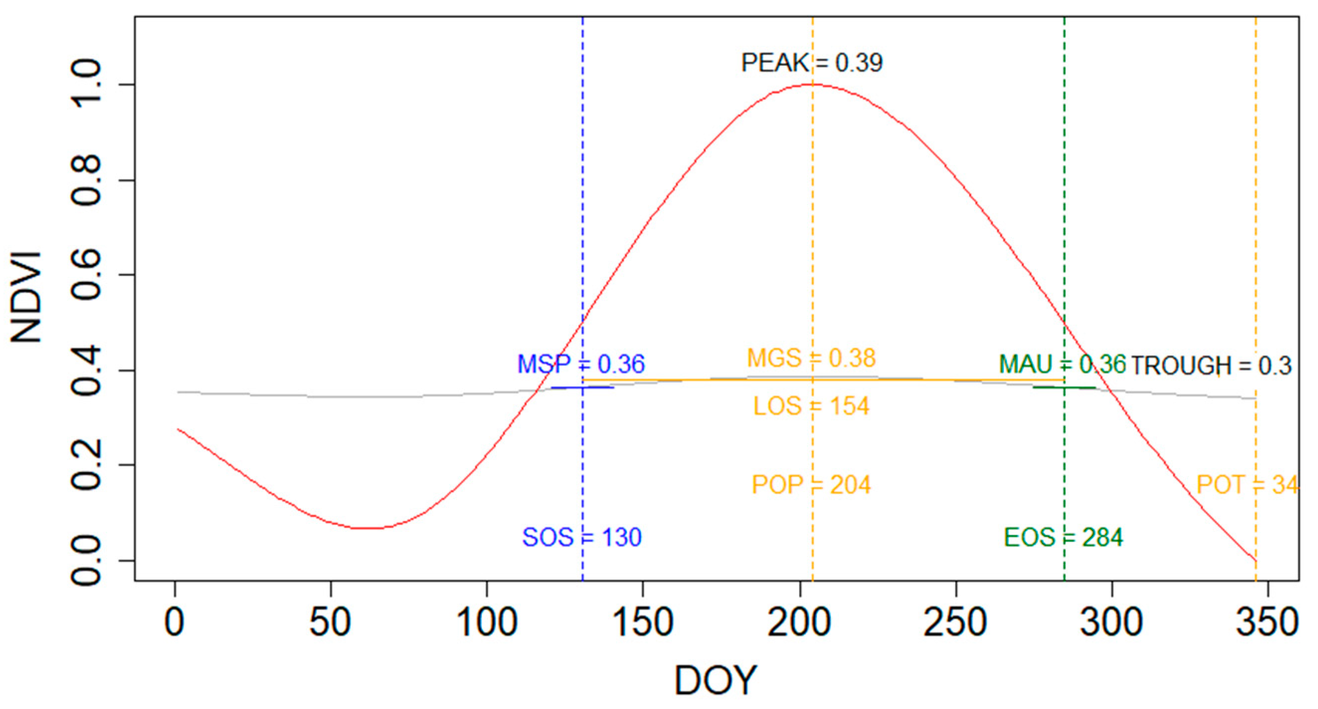
2.4. Phenology Extraction

Phenology metrics are very important indicators for ecosystem function, as delayed or advanced phenology metrics result in increased or decreased net primary production (NPP) which influences crop yield. Phenology mainly refers to the calculation of Start of Season (SOS), Length of Season (LOS), and End of Season (EOS) [71]. These phenology stages, however, are affected by varying degrees of drought, and we investigated the severity of drought for each phenology stage. As each crop growth stage has different water requirements–for example, vegetative, flowering, and grain filling stages are more sensitive to water–we extracted the period of SOS, LOS, and EOS to quantify the water deficit during these periods. Therefore, we decided to use the same periods of each phenology stage to calculate all drought indices. The phenology metrics were calculated in R software using the greenbrown package [72]. For example, the SOS, LOS, and EOS extracted from the smoothed time series NDVI in R software varies from March to May, May to August, and September to October, respectively, from 2001–2016 over South Asia. Thus, monthly drought indices values (VCI, TCI, VHI, SMDI, EDI, PAI, PCI, SPI-3, SPI-6, SPEI-3, SPEI-6) between SOS, LOS, and EOS for each pixel were used to obtain individual years’ drought status. To calculate the phenology metrics, the seasonality parameters were checked and extracted using a fast Fourier transformation of the time series NDVI data from GIMMS-NDVI (Global Inventory Modeling and Mapping Studies-NDVI). The tsgf (temporal smoothing and gap-filling) method was applied for temporal smoothing, which uses the derivative method taking into account the minimum mean annual value of each grid cell to determine SOS, LOS and EOS. Average phenology metrics extracted from the smoothed NDVI are presented in Figure 3.

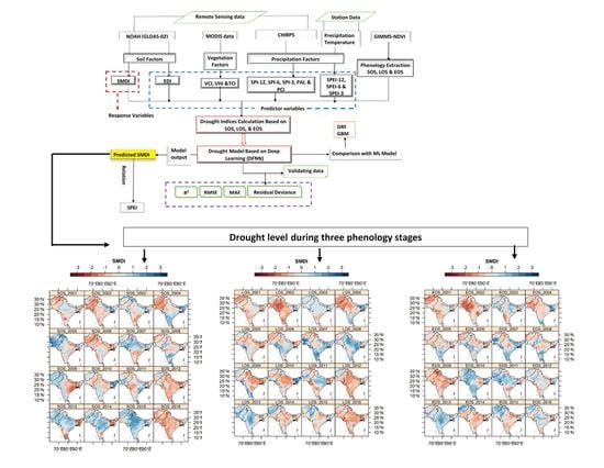
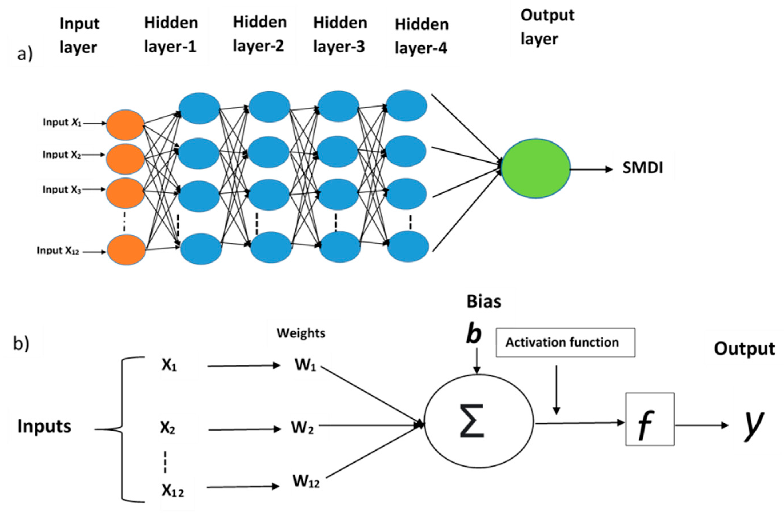
2.5. Construction of Deep Learning Model Using DFNN

Deep learning is recognized as part of machine learning, capable of solving complex tasks in the form of object detection, feature selection, image classification, and decision making [73]. Deep learning varies from conventional neural networks in that it utilizes many layers and several hidden layers, whereas a traditional neural network utilizes just two to three layers [74,75]. In the present study, we used the H2O package, which was designed for DFNN as a deep learning model to use in the R software [74]. DFNN, a supervised learning model with error back-propagation, can be found in detail at https://docs.h2o.ai/h2o/latest-stable/h2o-docs/data-science/deep-learning.html (accessed on 27 September 2020). DFNN, also known as Feed Forwarded Neural Network (FFNN), approximates the function by learning the value of the parameters. In this way, information passes from the input nodes through hidden layers to the output layers, indicating a one-way direction with no loops in the network. Our model was a multi-layer perceptron interconnected in a feed-forward way with one input layer containing the 12 explanatory variables (predictor variables), 4 hidden layers each of 300 nodes, and an output layer (response variable) (Appendix A). A drought-monitoring model was constructed based on DFNN considering SMDI as the function of precipitation, vegetation and soil factors as presented in Equation (1). Therefore, we employed 12 drought indices as input parameters to reflect the complex interaction between precipitation, vegetation, and soil factors.

Model Y = f (precipitation, vegetation, soil)

(1)

where Y = SMDI; precipitation = PAI, PCI, SPI-3, SPI-6, SPEI-3, SPEI-6; vegetation = VCI, VHI, TCI; and soil = EDI. In the present study, for each input variable a raster image of 7818 (row) × 8859 (column) dimension with a total pixel cell of 69259662 was used. Each pixel cell of a raster image represents the value of a corresponding input variable. Thus, the total size of the data is 69,259,662 for each input variable was used in the deep leaning model. First, the data set was randomly split into three parts, i.e., (i) training data (75% of the total sample), (ii) validation data (12.5% of the total sample), and (iii) test data (12.5% of the total sample). Generally, a training data set is used to fit the model with weights and biases in the case of a neural network. The model also learns from the training data set. Validation data is a sample of data used for unbiased evaluation of model fit while tuning model parameters on the training data set. Alternatively, the evaluation of the final model fit is usually done with a test data set. We applied the same data partition for 16 years (2001–2016). We calibrated the model by tuning different parameters of the model on the training data set, and the model results were validated using cross validation (a resampling procedure of the data set used to validate the model in order to estimate how the model is expected to perform) data. Further, we statistically compared the model’s performance on the test data set.

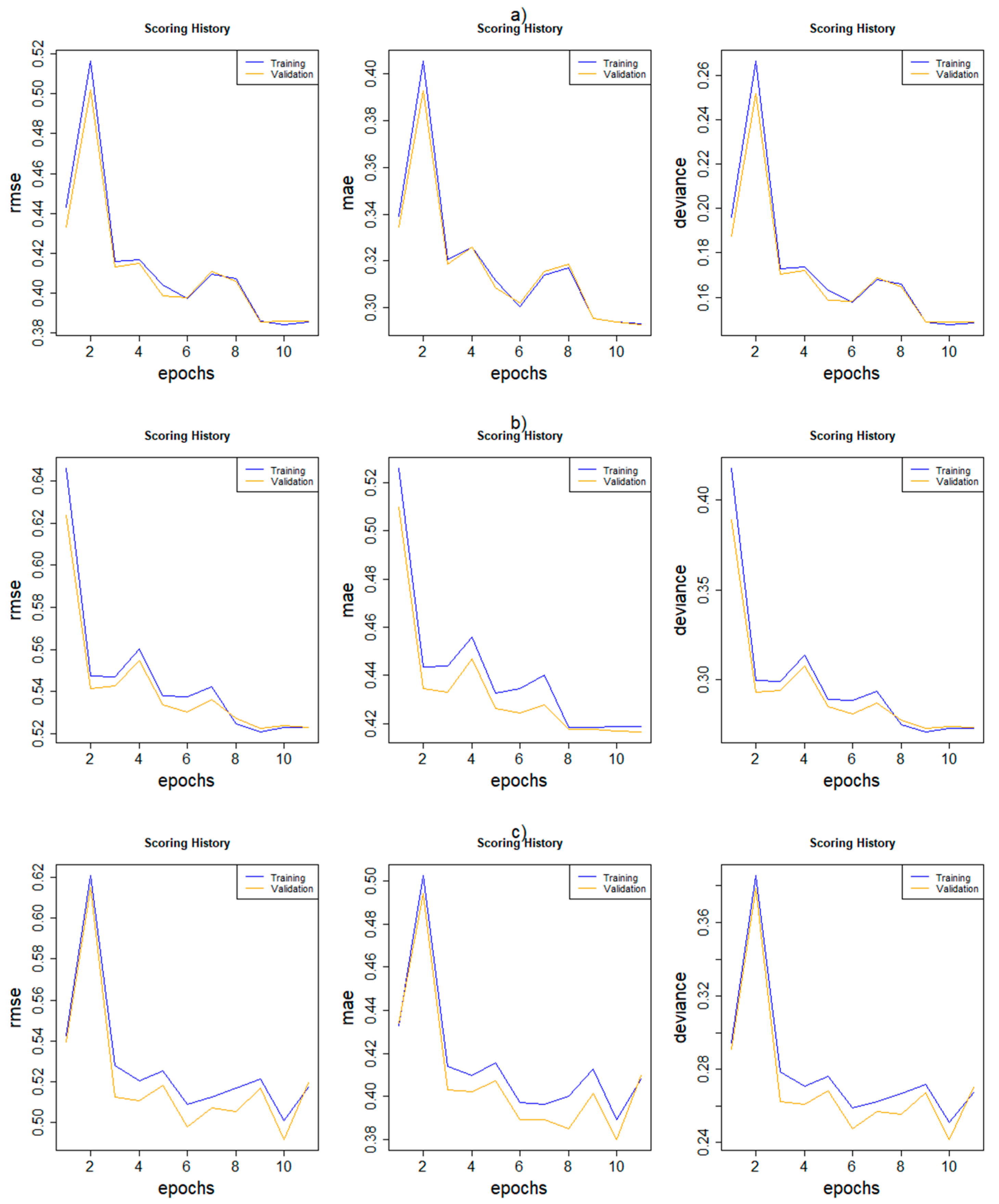
2.6. Model Calibration on Training Data Set by Tuning Model Parameter

To obtain the optimal structure of a DFNN model, the number of hidden layers and nodes setup is a crucial factor, as the model’s performance and accuracy largely depends on the size of the data set and model parameters. First, we used the default parameter of the H2O package to build neural networks which include the ‘Rectifier’ activation function with 200 neurons and 10 epoch (number of passes over the training data set to be carried out). In addition, the L1 and L2 regulation (representing the sum of square of all weights and biases in the network) used to prevent overfitting were assigned to a default value of 0. The hidden drop-out ratio that permits a large number of the models to be averaged as an ensemble was fixed to a default value of 0. Then, we examined model performance with the above-mentioned input parameters by enabling early stopping, which stops training when the model reaches a certain validation error. In order to obtain low RMSE, MAE, and mean deviance with a high R² value, we increased the number of neurons from 200 to 300, L1 and L2 0 to 1 × 10⁻⁶, hidden drop out ratio of 0 to 0.2 after each iteration, with epoch remaining at 10. The ‘max_W2’ (a maximum sum of squared incoming weights into anyone neuron) parameter, useful for unbound activation function, was also added with a value of 10. The ‘max_W2’ function introduces bias into parameter estimates, but frequently produces substantial gains in modeling as estimate variance is reduced, which enables high predictive accuracy. Moreover, the activation function was changed from ‘Rectified leaner unit’ to ‘RectifierWithDropout’ (‘Rectified leaner unit’ and ‘RectifierWithDropout’ represent non-linear activation functions) to activate the neurons more actively. We obtained minimum error for each of the performance metrics (RMSE, MAE, and deviance) when the data set irritated 10 times with 300 neurons, presented in Figure 4. We highlighted the scoring statistics considering drought severity for the year of 2012 as the same input parameters were applied for the rest of the years, hence why discussion of all years is not necessary. Further, we demonstrated the scoring history of the DFNN model at three phenology stages. Though there were some differences, the scoring trend both in training and validation data were similar. We observed, during the SOS stage, after starting the model, that the error increased sharply then decreased sharply, with some upward and downward curves as the model progressed (Figure 4a). Error became flat at epoch 10 for both data sets, demonstrating a low error rate. However, quite the opposite scenario was found at the LOS stage, which showed a sharply decreasing curve after starting the iteration. It became somewhat flat at epoch 10, though an upward and downward curve is observed between 3–8 epochs (Figure 4b). In the case of the EOS stage, the model initially showed a similar pattern to that seen in SOS, and then after the 10^th learning time, the error values were likely at a minimum compared to other learning times (Figure 4c). After calibration of the DFNN model, we obtained R² for training and validation data set, as shown in

Table 4. Scoring performance of DFNN model at each iteration during the different phenological stage.

Epoch	Samples			Training Speed (obs/sec)			Training-R2			Validation-R2
	SOS	LOS	EOS	SOS	LOS	EOS	SOS	LOS	EOS	SOS	LOS	EOS
1	5501	5499	5500	592	595	768	0.622	0.550	0.684	0.749	0.555	0.689
2	11,002	10,998	11,000	671	696	861	0.575	0.565	0.737	0.703	0.569	0.737
3	16,503	16,497	16,500	724	766	929	0.643	0.608	0.755	0.770	0.611	0.745
4	22,004	21,996	22,000	770	820	989	0.502	0.757	0.744	0.523	0.762	0.742
5	27,505	27,495	27,500	808	866	1041	0.694	0.808	0.759	0.720	0.801	0.752
6	33,006	32,994	33,000	840	902	1084	0.778	0.870	0.784	0.816	0.873	0.775
7	38,507	38,493	38,500	871	937	1114	0.791	0.875	0.762	0.817	0.878	0.749
8	44,008	43,992	44,000	900	970	1151	0.798	0.881	0.769	0.815	0.878	0.754
9	49,509	49,491	49,500	929	1001	1185	0.801	0.889	0.784	0.818	0.880	0.775
10	55,010	54,990	55,000	956	1030	1216	0.811	0.891	0.793	0.830	0.892	0.778
11	60,511	60,489	60,500	981	1039	1244	0.809	0.881	0.778	0.828	0.886	0.761

. Our model produced low R² for training and validation data set with fewer epochs, and a gradually higher R² value occurred with increasing epoch numbers. The results of the model had a good agreement with R² values of 0.811, 0.891, and 0.793 during SOS, LOS, and EOS stages, respectively, with epoch number 10. These findings indicate that a model with a large number of epochs facilitates better learning of the training data set and, in turn, better prediction results.

2.7. Model Validation Using Cross-Validation Data

We validated the DFNN model internally using a cross-validation method that permitted us to examine how well a model learned, i.e., the stability of the network structure. A number of 5 to 10 is considered good for K-folds cross-validation, and we selected the value for K as 10. The data were randomly split for 10 fold cross-validation. All 10 cross-validation models were formed based on 90% of the training data and 10% of the validation data. The model computed validation metrics for every 10 cross-validations by scoring against the true levels of 20% validation data. As a result, to make one prediction, 10 validation predictions are merged, and in this way overall cross-validation metrics are computed. The outcome of the DFNN model cross-validation metrics is presented in Figure 5. Figure 5 demonstrated high R² value ranges from 0.77 to 0.80, 0.86 to 0.90, and 0.75 to 0.80 for the periods of SOS, LOS, and EOS phonology stages, respectively. A high R² value indicates a low error rate which is presented as RMSE (mean value for SOS = 0.32, LOS = 0.31, and EOS = 0.44), MAE (mean value for SOS = 0.41, LOS = 0.22, and EOS = 0.33), and residual deviance (mean value for SOS = 0.17, LOS = 0.09, and EOS = 0.19) metrics by cross-validation analysis. Overall results suggested that the parameter used for the DFNN model was stable enough to reflect the high accuracy of the model for drought monitoring.

2.8. Machine Learning Model

Apart from deep learning, two machine learning models, DRF and GBM, were used. These two machine learning algorithms are flexible and robust for classification and regression tasks [16]. DRF is a tree-based algorithm that produces a forest of trees rather than a single tree that uses a randomized subset of candidate features by applying bootstrap sampling to make a final prediction [51]. GBM is also tree-based, using forward-learning ensemble methods that build a regression tree on all features of the data set for building a predictive model. It works by optimizing the loss function using a weak learner to make a prediction, and by applying an additive model the loss function is minimized. We used the H2O package for DRF and GBM analysis in the R software. To obtain optimum performance, we kept the same value for some important parameters such as ‘number of trees’, ‘max. depth’, ‘learn_rate’, ‘sample_rate’, fold_assignment = “Random” etc. for both the DRF and GBM models. The important parameters with their choice of values are present in Appendix B.

2.9. Mann-Kendall Test for Drought Trend Analysis

The rank-based Mann–Kendall method, a nonparametric test, was applied to track the increasing and decreasing trends of drought over South Asia at the pixel level during 2001–2016. The Mann–Kendall test, expressed by Mann [76] and explained by Kendall [77], is commonly used for trend detection in the case of time series of environmental, climate and hydrological data [78,79], as well as droughts and aridities of very different spatiotemporal ranges in other very remote regions [80,81]. In general, the Mann–Kendal test follows a monotonic trend rather than a strictly linear trend [82]. The magnitude of the trend was detected by Shen’s slope estimator [83] to calculate the upward and downward change of drought levels. A slope with a positive value indicates an increasing trend, while negative values represent a decreasing trend. The equation of Shen’s slope is as follows:

$$\beta =mean\left(\frac{x^j-x^i}{j-i}\right)j>i$$

(2)

In Equation (2), β is the trend of SMDI, i and j indicate the interval of the time series, and $x^i$ and $x^j$ indicate the SMDI value for the year between i and j. The Mann–Kendall test was performed using ‘spatialEco’ package in R software [84].

3. Results

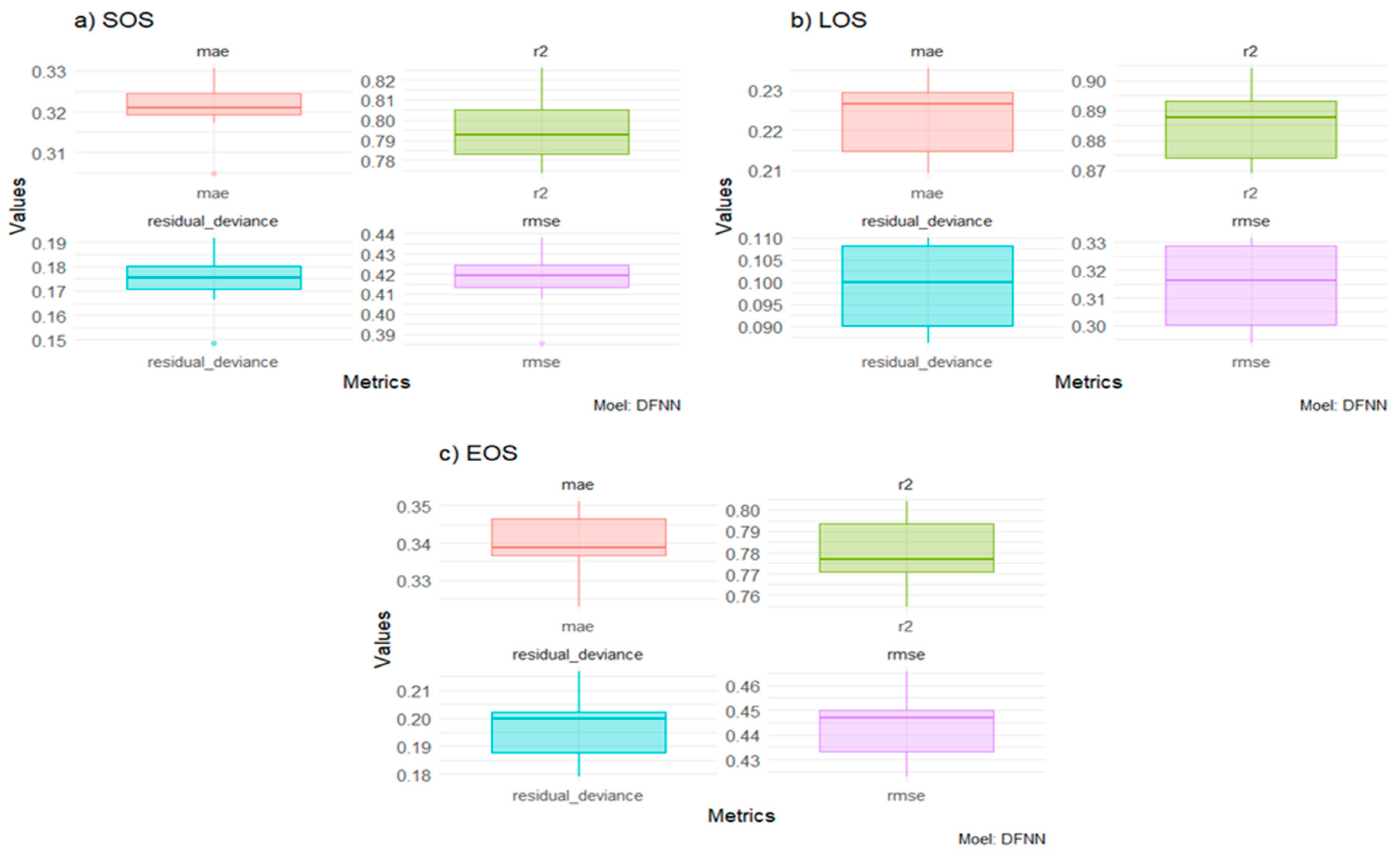
3.1. Deep Learning and Machine Learning Model Performance with Observed Data and Its Statistical Comparison Using Test Data Set in Detecting Drought Pattern

The discrimination between the deep learning and machine learning approaches for drought distribution in terms of spatial pattern over South Asia is presented in Figure 6. We also observed and compared the spatiotemporal change of drought conditions at three phenology stages during the 2012 drought year, taking drought severity into account. Both deep learning and two machine learning models show relatively low SMDI levels during the SOS and LOS compared to the EOS stage. The northern and southwestern parts of India, Bangladesh, and Nepal had more dry soil during SOS and LOS stages. However, EOS representing drier soil in the southwestern part of India and the northwestern part of Bangladesh. When compared to the observed SMDI distribution, the DFNN and GBM models captured a nearly identical drought pattern. Simultaneously, SMDI levels were underestimated by the DRF model compared to the observed SMDI pattern over the South Asia region. It is evident that at three phenology stages DFNN and GBM caught similar SMDI patterns and well-matched with observed SMDI in terms of spatial distribution over different parts of the South Asia region. To compare further, we statistically evaluated the predicted performance on the test between the deep learning and machine learning models in terms of RMSE, MAE, and MSE (mean square error) during three phenology stages (

Table 5. Comparison of the performance of deep learning and machine learning model on the test data set for the prediction of SMDI.

Phenology	Model	Test Data
		RMSE	MAE	MSE
SOS	DFNN	0.417	0.310	0.174
	GBM	0.439	0.330	0.193
	DRF	0.443	0.318	0.196
LOS	DFNN	0.486	0.359	0.237
	GBM	0.514	0.381	0.264
	DRF	0.517	0.399	0.268
EOS	DFNN	0.466	0.354	0.217
	GBM	0.501	0.378	0.251
	DRF	0.514	0.403	0.265

). Results presented in Table 5 indicate that DFNN showed better performance with low RMSE, MAE, and MSE than GBM and RF.

As we can see in Figure 7, the frequency distribution of SMDI is almost identical to that of the DFNN and GBM models. Still, less similarity was noticed in frequency distribution for the DRF model. The frequency distribution shows its peak SMDI value of −1.2 and −1.5 for both SOS and LOS stages, respectively. The frequency distribution curve was found in the EOS stage with a peak greater than 0 (0.3) for all models. The performance of deep learning and two machine learning models using a tailor diagram (DFNN, DRF, and RF) is presented in Figure 8. The Taylor diagram presented in Figure 8 reveals that DFNN and GBM performed well, demonstrating closer results to each other than the DRF model. Further, the DFNN and GBM model comparison shows that the DFNN performance is slightly better than the GBM model, even though the DFNN and GBM models capture almost similar spatial patterns to the observed data in estimating SMDI. This difference might be due to the multi-layer approach with high tuning parameters that makes computations more practical in the DFNN model than the shallow-depth GBM machine learning model, which has a comparatively low tuning parameter.

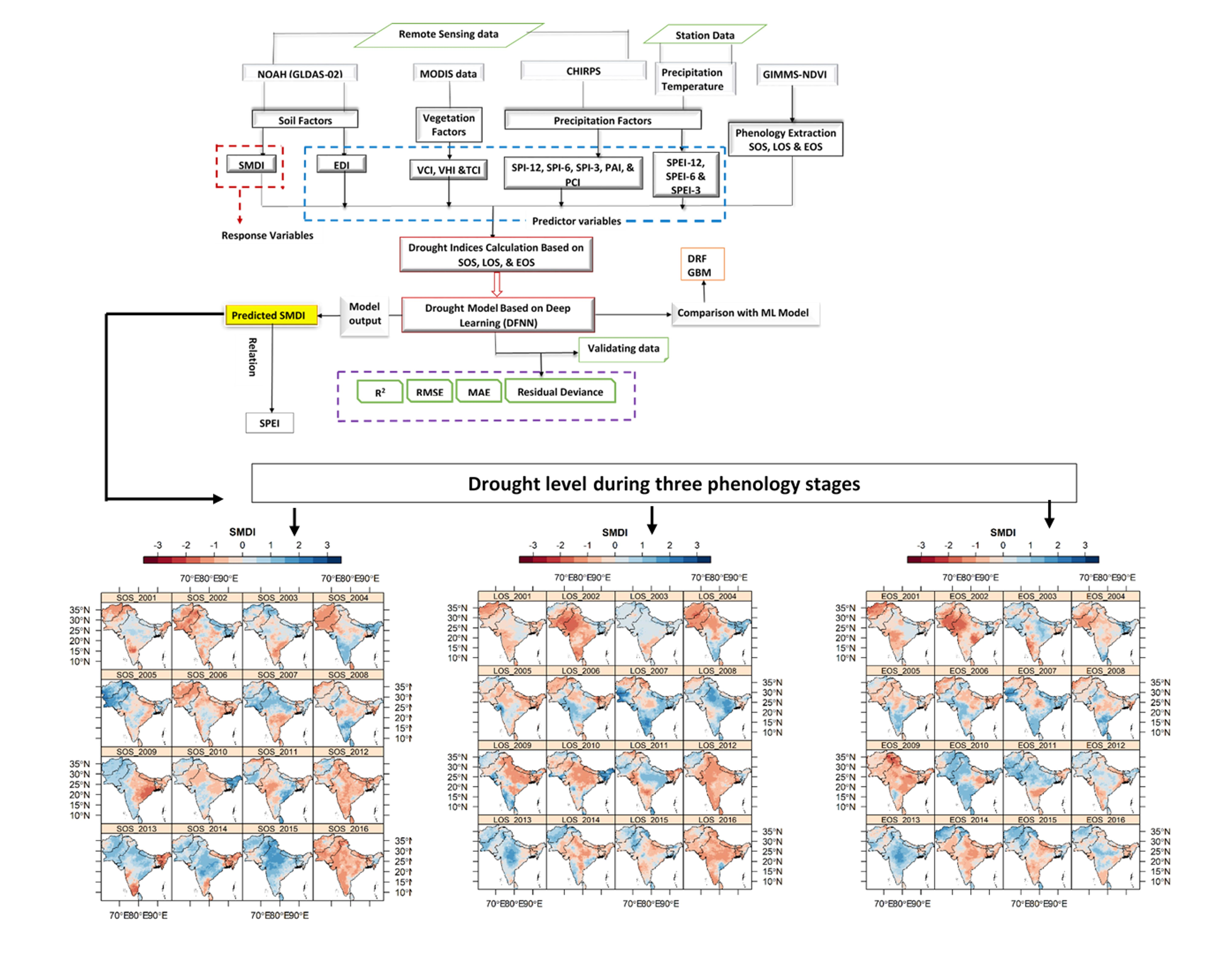
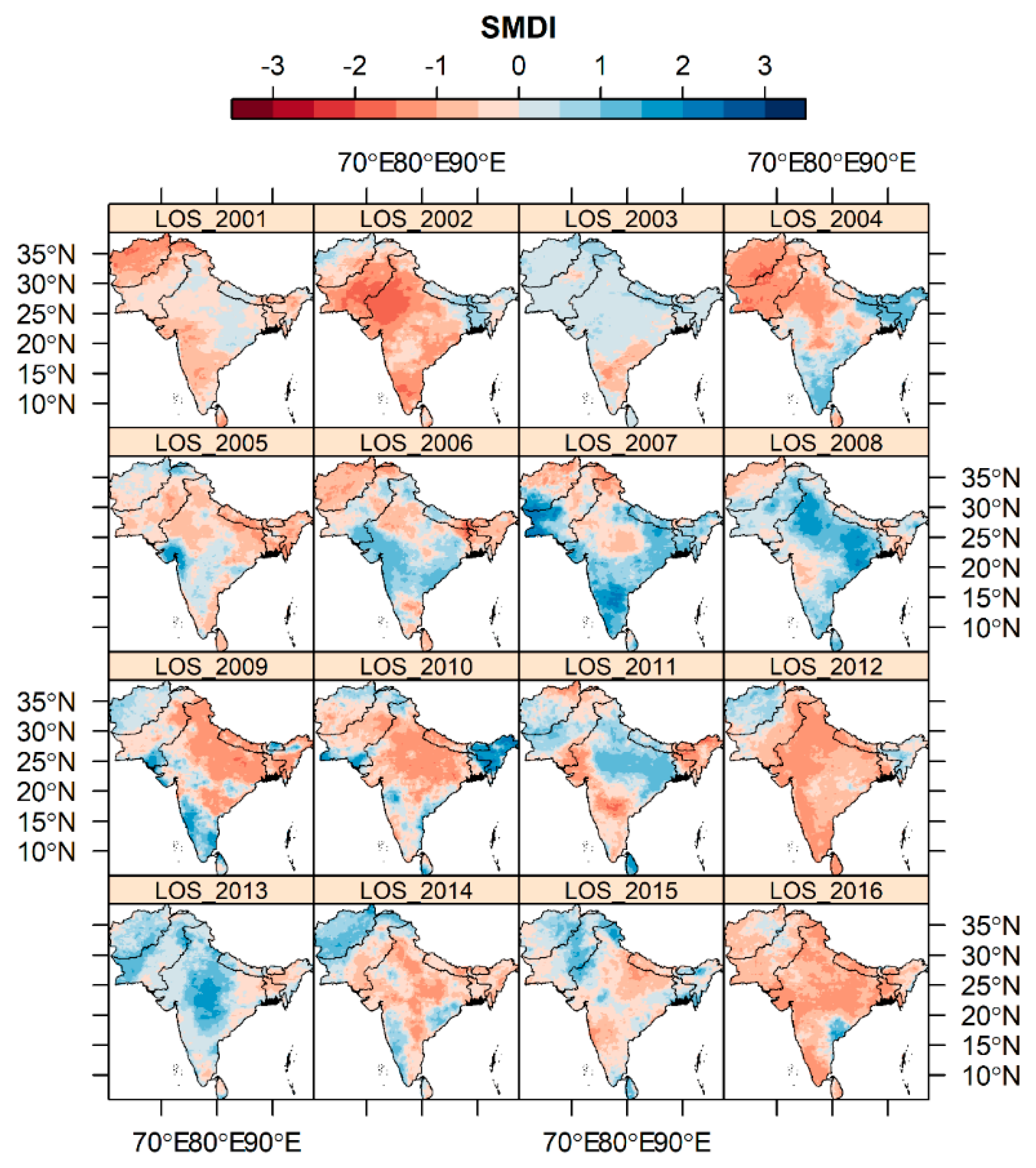
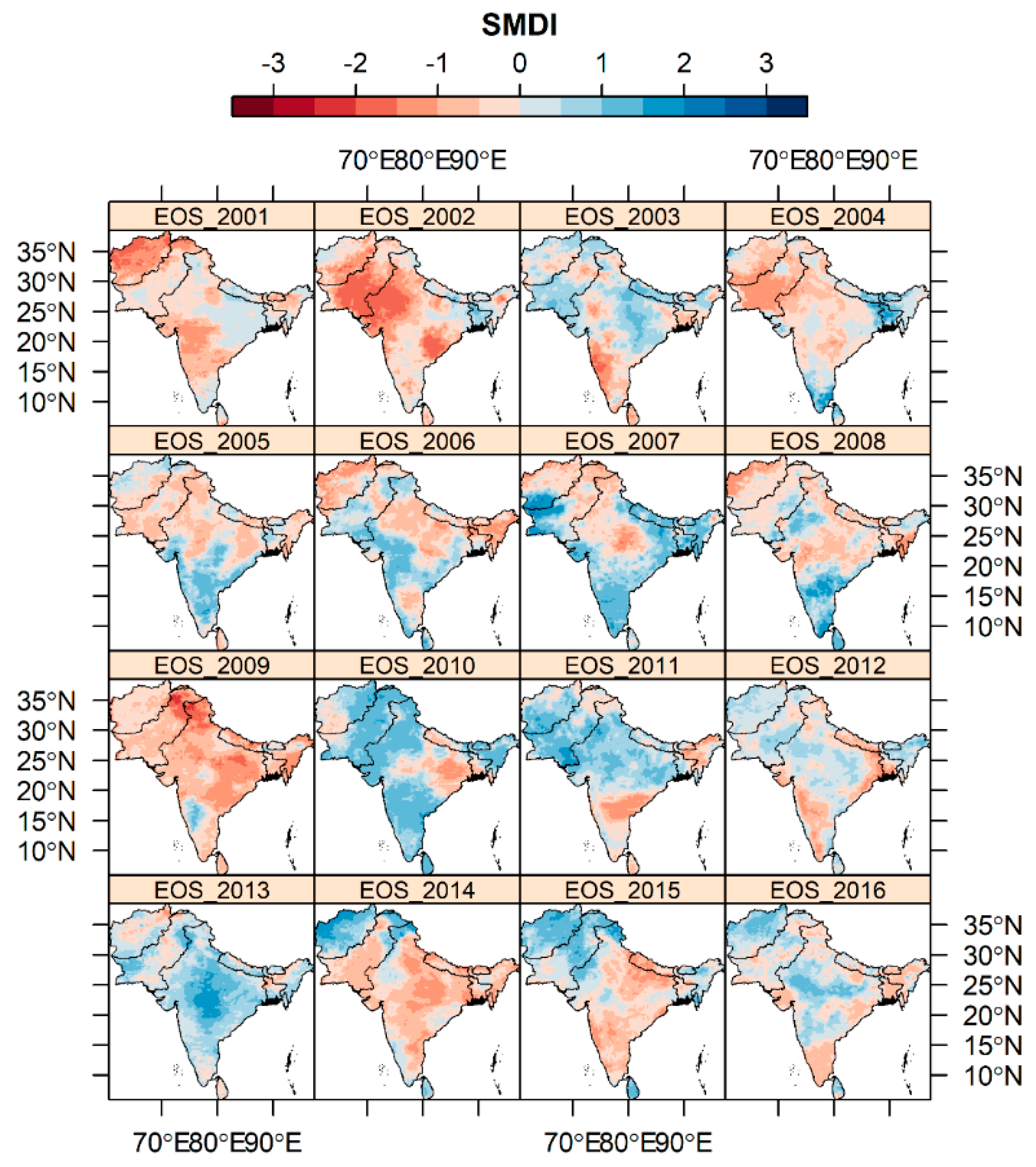
3.2. Spatiotemporal Pattern of Drought Based on SMDI Using a Deep Learning Model during Three Crop Phenology Stages

To study the effect of precipitation, soil, and vegetation factors on SMDI, we did a spatiotemporal analysis using a deep learning model. Spatially distributed SMDI with the impact of input model parameters was investigated during three phenology stages: SOS, LOS, and EOS. Figure 9, Figure 10 and Figure 11 show the evolution of drought during different phenology stages based on annual simulated SMDI values from the deep learning model over a 16-year period. The findings seem to expose that the severest yearly droughts for the South Asia region were found in 2002, 2006, 2012, and 2016 during SOS (Figure 9) whereas 2002, 2004, 2012, and 2016 saw severe drought for the duration of the LOS stage (Figure 10). However, drought that hit at the EOS stage is visible during 2001, 2002, 2009, and 2014 (Figure 11). Overall, the spatial agreement coming from the results of the deep learning model shows high stability of SMDI values at three phenology stages. This high spatial agreement of SMDI is demonstrative of precipitation, vegetation, and soil factors on drought patterns over the South Asia region, which derives from the simulation of the deep learning model.

The trend of drought over South Asia during three phenology stages was estimated based on the Mann–Kendal test from 2001–2016, as shown in Figure 12. The spatiotemporal pattern of increasing and decreasing drought trend (Figure 12a) and the corresponding significant level (Figure 12b) demonstrated that drought spatially increases in the central part of Afghanistan and Northwestern part of Pakistan during SOS and LOS stages. Alternatively, Afghanistan, central Pakistan, and the northwestern part of India demonstrated an increasing drought trend during the EOS stage. The erratic rainfall pattern with high potential evapotranspiration causes a significant increasing trend of drought for the region mentioned above. However, the southeastern and southwestern parts of Nepal and northern parts of Bangladesh show a significant decreasing agricultural drought trend due to high rainfall during the pre-monsoon and monsoon seasons.

For a clear understanding, we have plotted the observed and predicted SMDI during three phenology stages from 2001–2016 (Figure 13). The performance of SMDI against the observed SMDI data demonstrates high accuracy prediction. The plots of SMDI are a close to one to one (1:1) line that agrees well with the observed SMDI values. The predicted SMDI looks to be functioning better at the LOS (R2 = 0.52 to 0.94) than the SOS (R2 = 0.57 to 0.90) and EOS (R2 = 0.49 to 0.82) stages.

Further, we investigated how much each input variable stimulates the SMDI distribution over South Asia by exploring the variable importance feature to the input function of the deep learning model. Results presented in

Table 6. Contribution of each input variable to the output function of the model. The relative importance indicates how changes in the explanatory variables are linked to shifts in the response variable of the model and the percentage represent the corresponding contribution of the variables.

Variables	Relative Importance			Percentage
	SOS	LOS	EOS	SOS	LOS	EOS
SPI-6	1.0	1.0	1.0	15.60	20.40	19.30
SPI-3	0.918	0.671	0.578	8.18	9.40	6.16
SPI-12	0.538	0.435	0.451	6.62	4.30	5.14
SPEI-6	0.910	0.387	0.453	14.20	8.70	8.71
SPEI-3	0.457	0.323	0.440	4.12	4.38	5.33
SPEI-12	0.238	0.211	0.291	3.08	2.22	3.54
PCI	0.393	0.463	0.677	5.20	9.40	13.12
EDI	0.701	0.502	0.465	10.90	10.20	9.00
PAI	0.593	0.367	0.396	9.20	7.50	7.60
TCI	0.548	0.479	0.453	8.50	9.80	8.80
VHI	0.470	0.346	0.337	7.30	7.00	6.50
VCI	0.455	0.331	0.353	7.10	6.70	6.80

suggested that precipitation factors were the most important factors, contributing significantly to SMDI during the three phenology stages. In addition, among the precipitation factors SPI-6 had the highest contribution effects on SMDI variability simulated by the DFNN model.

In addition, we measured the marginal impact of SPI-6 in three phenology stages presented in Figure 14 with the H₂O partial plot function of the R program to understand how SPI-6 influences the spatial distribution of SMDI over South Asia. The spatial variability of SMDI followed the variability of SPI-6 to a great extent, indicating that with an increase in SPI-6 value, the SMDI value also increased. The relationship between SPI-6 and SMDI shows a linear trend that describes a unit change of SPI -6 value changes in soil moisture occurs. From the above findings, we can conclude that soil moisture- induced drought increases with a low precipitation rate.

We performed a temporal analysis that provided a reasonable estimate of drought severity for each phenology stage that is very sensitive to water stress (Figure 15) to understand how much each region is affected by drought. For example, droughts that hit the South Asia region are distinctly noticeable for the years of 2002, 2004, 2006, 2012, and 2016 affecting 21.22%, 22.99%, 23.82%, 23.57%, and 39.19%, respectively, of the total area during the SOS stage. Further notable drought was detected in South Asia in 2002, 2004, 2012, and 2016, affecting 42.9%, 33.9%, 33.4%, and 32.2% of the total area, respectively, during the LOS stage. However, comparatively less drought intensity was observed during the EOS stage, influencing 34.64%, 27.48% and 11.2% land of the total area, respectively, in 2002, 2009, and 2014. Furthermore, we also explored the relationship of SMDI simulated by the DFNN model with ground observed SPEI for the evaluation of inter-annual variability of SMDI concerning precipitation. Taking one of the drought-affected stations as an example, the temporal variation of SMDI and SPEI is presented in Figure 16 reveals that SMDI anomaly fluctuations matched well with those of SPEI-3 and SPEI-6 anomaly. Based on the analysis, it can be concluded that SMDI is well correlated with SPEI and SPEI shows a more significant effect on SMDI anomaly.

3.3. Uncertainties in SMDI Analysis by DFNN Model

Deep learning-based SMDI prediction is suitable for spatiotemporal drought information that helps government planners to make mitigation and adaptation strategies at the regional level. The deep learning model uses the observation weight column of each incoming data associated with neurons used for bias correction. Thus, the weight of each node determines the output of the entire network. However, the simulated results of drought by the deep learning model mainly depend on learning from past drought information, so an area with no experience of drought is challenging to predict for. Additionally, in our case we used different multi-sensors for remote sensing data with different spatial resolutions, which requires a large number of high-quality training images for better model learning. Moreover, the complexity of the high resolution remote sensing images includes various types of objects with different sizes, rotations, and formats in a single scene, requiring transformation to the same features which creates a problem of robust learning and discriminative illustrations from the objects with deep learning [85]. The above-mentioned causes lead to some uncertainties during the model simulation. For this, we calculated the bias that was generated during the training of the data for each neuron and investigated its spatial pattern (Figure 17). The bias of all neurons ranges from 0.20–0.55 for three phenology stages (Figure 17a–c). Furthermore, the spatial distribution of bias estimated by calculating the difference between model derived SMDI and observed SMDI presented in Figure 17d–f shows that most of the South Asia region had no bias or tended to zero, but some pixels of the northern and southern parts displayed overestimated and underestimated values compared to the observed values. To minimize bias, we need more training data with a more precise and accurate transformation of remote sensing for better model learning.

4. Discussion

4.1. Model Comparison and Performance

This study established the application of a deep learning model for monitoring drought over South Asia. We also used two machine learning models, DRF and GBM, to compare their performance against deep learning. In the case of capturing the spatial pattern of SMDI, the DRF model differs significantly compared to the observed SMDI due to high errors during the training of the data set for each iteration [16,86]. High learning rate and high speed in the case of big data set reduce estimation error for each iteration of the DFNN and GBM models compared to the DRF model, which leads the predicted pattern of SMDI trending towards the observed SMDI pattern. However, the overall performance of deep learning is better than the DRF and RF models because it tends to reduce estimation error with high accuracy due to a multi-layer neural network. Alternatively, DRF requires more computational demand owing to large tree size, which is one of the reasons for low performance over deep learning. Then again, GBM is a slow depth model that offers fewer advantages for dealing with multi-dimensional complex features than the deep learning model [87,88]. These differences might cause the error and low accuracy for predicting SMDI by the DRF and GBM models. Moreover, deep learning has the ability to find the optimal output in the case of high-dimensional data features due to its multi-layer approach. Additionally, many input parameters such as hidden layers with neurons, adaptive learning rate, grid search, dropout function etc. make the computation more practical, more relevant, and advance the underlying algorithms resulting in high predictive accuracy [85]. Sometimes even tree-based non-linear algorithms such as GBM and DRF fail to learn from the data. In that circumstance, deep neural architecture generates non-linear interaction among the variables due to its training stability, facilitating learning the entire network together [75,89].

4.2. Drought Variation in Three Phenology Stages

In reality, most of the South Asia region persisted a dry condition and suffered from moderate to severe drought, based on drought classifications presented in Table 1, at three phenology stages during the above-mentioned drought years (presented in Section 3.2). Our findings are consistent with the results reported by Mujumdar et al. [90], Neena et al. [91], and Krishnan et al. [92] in which moderate to severe drought in the Indian sub-continent for the years 2002, 2004, 2009, 2014, and 2016 was noticed. The persistence of low soil moisture during the different phenology stages is associated with low precipitation, which brings changes in hydrology and water availability in soil particles. The low precipitation involved with the EI Nino condition over the northwest and northcentral pacific leads to monsoon rainfall deficiency in the South Asia region. Drought most affected the SOS and LOS stages, compared to the EOS stage. SOS is mainly the onset of the monsoon season characterized by a hot summer, which suffers from insufficient rainfall, whereas the LOS stage lasts for the monsoon season with hot and humid conditions, which is also influenced by low rainfall due to Indian Ocean Oscillation and the sea surface temperature gradient between the Indian Ocean and the Bay of Bengal [93,94]. As a result, seasonal drought occurs in SOS and LOS stages. In contrast, the EOS stage, which is the post-monsoon season period, experienced comparatively fewer drought phenomena because the soil particles hold the water that comes from rainfall during the monsoon season. Further, drought gradually expanded from SOS to the LOS stage because crop water requirements reached high levels during LOS due to a rapid increase in the crops’ vegetative growth. In addition, high evapotranspiration with rising temperature makes the LOS stage more vulnerable to drought conditions. However, the regional variation of drought trend over South Asia is mainly attributed to the high variability of temperature and rainfall associated with faster changing of the warming phase in the Indian Ocean [95].

4.3. SMDI Prediction and Drought Severity Assessment

The SMDI drought index is very robust to short-term dry conditions and very comparable across the season that estimated well the dry conditions in the three phenology stages (SOS, LOS, and EOS), which represents agricultural drought. It is also spatially comparable and varies from one phenology stage to other stages because SMDI is derived from historical value, and the calculation is independent at each grid cell. Though drought affects a large area of each phenology stage, dry and wetness conditions are primarily region-specific, based on precipitation, land cover type, soil texture, and water holding capacity [96,97,98]. The country-level analysis shows the severity of local droughts in India, Pakistan, and Afghanistan during the three phenology stages. This result might be due to the moderate El Niño condition with irregular atmospheric convective activity over the north-central Pacific, which caused rainfall insufficiency over the Indian subcontinent [99,100,101]. Moreover, extended monsoon breaks in the Indian Ocean triggered by ocean-atmosphere dynamical coupling on the intra-seasonal time scale generates drought over the Indian sub-continent [92,102]. The continental- and country-scale analysis aids in understanding the magnitude of local droughts, which may aid in policy formation for post-disaster management to mitigate drought’s impact on natural resources.

5. Conclusions

The present study explored the applicability of a deep learning model to monitor agricultural drought using remote-sensing data. The skill of the model was evaluated using cross-validation data during the training phase of the model. Additionally, the inter-annual variability of the SMDI was investigated using ground observation data measured with SPEI. The results suggested that the DFNN model was the most-capable tool for monitoring drought across South Asia during three phenology stages. The DFNN model outperformed the other two DRF and GBM models considering precipitation, soil, and vegetation factors. The simulated SMDI by the DFNN model had good consistency with the observed SMDI, and it also matched well with SPEI. The DFNN model estimated yearly drought intensity with high spatial variability across the three phenology stages. The spatial variability was attributed mainly due to the precipitation variability that was examined by the model using relative importance features. Results suggested that droughts in the South Asia region are clearly evident for the years of 2002, 2004, 2006, 2012, and 2016 influencing 21.22%, 22.99%, 23.82%, 23.57% and 39.19% respectively of the total area during the SOS stage while, during LOS stage, 42.9%, 33.9%, 33.4%, and 32.2% of the total area was affected by drought in the years of 2002, 2004, 2012, and 2016 respectively. Alternatively, a reasonably less drought intensity was found during the EOS stage, which caused soil dryness for the years 2002, 2009 and 2014, affecting 34.64%, 27.48% and 11.2% of the total area. The drought prediction system using a deep learning approach facilitates improving agricultural drought monitoring capability over South Asia during crop phenology stages. Moreover, that this study provides a guide of necessity to adopt adaptation strategies or improved management practices by understanding the risk of drought in each crop growing month is one of our contributions. However, the effectiveness and operational ability of the model depend on model input parameters and the size of the training data set. In this regard, incorporation of more drought factors as input parameters with remote sensing-based approaches to meteorological and hydrological drought using different hybrid models could be a future research approach.

References

1. Heim, R.R., Jr. A Review of Twentieth-Century Drought Indices Used in the United States. Bull. Am. Meteorol. Soc. 2002, 83, 1149–1166. [Google Scholar] [CrossRef] [Green Version]
2. Dai, A. Drought under global warming: A review. Wiley Interdiscip. Rev. Clim. Chang. 2011, 2, 45–65. [Google Scholar] [CrossRef] [Green Version]
3. Hao, Z.; AghaKouchak, A.; Nakhjiri, N.; Farahmand, A. Global integrated drought monitoring and prediction system. Sci. Data 2014, 1, 140001. [Google Scholar] [CrossRef]
4. Aadhar, S.; Mishra, V. Data Descriptor: High-resolution near real-time drought monitoring in South Asia. Sci. Data 2017, 4, 170145. [Google Scholar] [CrossRef] [PubMed] [Green Version]
5. Wilhite, D.A.; Hayes, M.J.; Knutson, C.L. Drought and Water Crises: Science, Technology, and Management Issues; CRC Press: Boca Raton, FL, USA, 2005; ISBN 9781420028386. [Google Scholar]
6. Esfahanian, E.; Nejadhashemi, A.P.; Abouali, M.; Adhikari, U.; Zhang, Z.; Daneshvar, F.; Herman, M.R. Development and evaluation of a comprehensive drought index. J. Environ. Manag. 2017, 185, 31–43. [Google Scholar] [CrossRef] [PubMed] [Green Version]
7. Zhang, J.; Zhou, Z.; Yao, F.; Yang, L.; Hao, C. Validating the modified perpendicular drought index in the North China region using in situ soil moisture measurement. IEEE Geosci. Remote Sens. Lett. 2015, 12, 542–546. [Google Scholar] [CrossRef]
8. Tadesse, T.; Champagne, C.; Wardlow, B.D.; Hadwen, T.A.; Brown, J.F.; Demisse, G.B.; Bayissa, Y.A.; Davidson, A.M. Building the vegetation drought response index for Canada (VegDRI-Canada) to monitor agricultural drought: First results. GISci. Remote Sens. 2017, 54, 230–257. [Google Scholar] [CrossRef]
9. Bhat, G.S. The Indian drought of 2002—A sub-seasonal phenomenon? Q. J. R. Meteorol. Soc. 2006, 132, 2583–2602. [Google Scholar] [CrossRef]
10. Mishra, V.; Aadhar, S.; Asoka, A.; Pai, S.; Kumar, R. On the frequency of the 2015 monsoon season drought in the Indo-Gangetic Plain. Geophys. Res. Lett. 2016, 43, 12102–12112. [Google Scholar] [CrossRef]
11. Ali, S.; Henchiri, M.; Yao, F.; Zhang, J. Analysis of vegetation dynamics, drought in relation with climate over South Asia from 1990 to 2011. Environ. Sci. Pollut. Res. 2019, 26, 11470–11481. [Google Scholar] [CrossRef]
12. Ahmad, S.; Hussain, Z.; Qureshi, A.S.; Majeed, R.; Saleem, M. Drought Mitigation in Pakistan: Current Status and Options for Future Strategies, 3nd ed.; International Water Management Institute: Colombo, Sri Lanka, 2004. [Google Scholar]
13. Dey, N.; Alam, M.; Sajjan, A.; Bhuiyan, M.; Ghose, L.; Ibaraki, Y.; Karim, F. Assessing Environmental and Health Impact of Drought in the Northwest Bangladesh. J. Environ. Sci. Nat. Resour. 2011, 4, 89–97. [Google Scholar] [CrossRef]
14. Ali, S.; Tong, D.; Xu, Z.T.; Henchiri, M.; Wilson, K.; Siqi, S.; Zhang, J. Characterization of drought monitoring events through MODIS- and TRMM-based DSI and TVDI over South Asia during 2001–2017. Environ. Sci. Pollut. Res. 2019, 26, 33568–33581. [Google Scholar] [CrossRef] [PubMed]
15. Feng, P.; Wang, B.; Liu, D.L.; Yu, Q. Machine learning-based integration of remotely-sensed drought factors can improve the estimation of agricultural drought in South-Eastern Australia. Agric. Syst. 2019, 173, 303–316. [Google Scholar] [CrossRef]
16. Park, S.; Im, J.; Jang, E.; Rhee, J. Drought assessment and monitoring through blending of multi-sensor indices using machine learning approaches for different climate regions. Agric. For. Meteorol. 2016, 216, 157–169. [Google Scholar] [CrossRef]
17. Quiring, S.M.; Ganesh, S. Evaluating the utility of the Vegetation Condition Index (VCI) for monitoring meteorological drought in Texas. Agric. For. Meteorol. 2010, 150, 330–339. [Google Scholar] [CrossRef]
18. Hao, C.; Zhang, J.; Yao, F. Combination of multi-sensor remote sensing data for drought monitoring over Southwest China. Int. J. Appl. Earth Obs. Geoinf. 2015, 35, 270–283. [Google Scholar] [CrossRef]
19. Liu, Q.; Zhang, S.; Zhang, H.; Bai, Y.; Zhang, J. Monitoring drought using composite drought indices based on remote sensing. Sci. Total Environ. 2020, 711, 134585. [Google Scholar] [CrossRef]
20. Yin, J.; Zhan, X.; Hain, C.R.; Liu, J.; Anderson, M.C. A Method for Objectively Integrating Soil Moisture Satellite Observations and Model Simulations Toward a Blended Drought Index. Water Resour. Res. 2018, 54, 6772–6791. [Google Scholar] [CrossRef]
21. Chen, J.; Li, M.; Wang, W. Statistical uncertainty estimation using random forests and its application to drought forecast. Math. Probl. Eng. 2012, 2012, 915053. [Google Scholar] [CrossRef] [Green Version]
22. Li, J.; Zhou, S.; Hu, R. Hydrological drought class transition using SPI and SRI time series by loglinear regression. Water Resour. Manag. 2016, 30, 669–684. [Google Scholar] [CrossRef]
23. Khadr, M. Forecasting of meteorological drought using Hidden Markov Model (case study: The upper Blue Nile river basin, Ethiopia). Ain Shams Eng. J. 2016, 7, 47–56. [Google Scholar] [CrossRef] [Green Version]
24. Morid, S.; Smakhtin, V.; Bagherzadeh, K. Drought forecasting using artificial neural networks and time series of drought indices. Int. J. Climatol. 2007, 27, 2103–2111. [Google Scholar] [CrossRef]
25. Shen, R.; Huang, A.; Li, B.; Guo, J. Construction of a drought monitoring model using deep learning based on multi-source remote sensing data. Int. J. Appl. Earth Obs. Geoinf. 2019, 79, 48–57. [Google Scholar] [CrossRef]
26. Narasimhan, B.; Srinivasan, R. Development and evaluation of Soil Moisture Deficit Index (SMDI) and Evapotranspiration Deficit Index (ETDI) for agricultural drought monitoring. Agric. For. Meteorol. 2005, 133, 69–88. [Google Scholar] [CrossRef]
27. Yang, S.; Meng, D.; Gong, H.; Li, X.; Wu, X. Soil Drought and Vegetation Response during 2001–2015 in North China Based on GLDAS and MODIS Data. Adv. Meteorol. 2018, 2018. [Google Scholar] [CrossRef] [Green Version]
28. Lecun, Y.; Bengio, Y.; Hinton, G. Deep learning. Nature 2015, 521, 436–444. [Google Scholar] [CrossRef]
29. Borji, M.; Malekian, A.; Salajegheh, A.; Ghadimi, M. Multi-time-scale analysis of hydrological drought forecasting using support vector regression (SVR) and artificial neural networks (ANN). Arab. J. Geosci. 2016, 9, 725. [Google Scholar] [CrossRef]
30. Zhang, A.; Jia, G.; Wang, H. Improving meteorological drought monitoring capability over tropical and subtropical water-limited ecosystems: Evaluation and ensemble of the Microwave Integrated Drought Index. Environ. Res. Lett. 2019, 14, 44025. [Google Scholar] [CrossRef]
31. Chiang, J.L.; Tsai, Y.S. Reservoir drought prediction using support vector machines. Appl. Mech. Mater. 2012, 145, 455–459. [Google Scholar] [CrossRef]
32. Lee, C.S.; Sohn, E.; Park, J.D.; Jang, J.D. Estimation of soil moisture using deep learning based on satellite data: A case study of South Korea. GISci. Remote Sens. 2019, 56, 43–67. [Google Scholar] [CrossRef]
33. Zhang, D.; Zhang, W.; Huang, W.; Hong, Z.; Meng, L. Upscaling of surface soil moisture using a deep learning model with VIIRS RDR. ISPRS Int. J. Geo-Inf. 2017, 6, 130. [Google Scholar] [CrossRef]
34. Agana, N.A.; Homaifar, A. A deep learning based approach for long-term drought prediction. In Proceedings of the SoutheastCon 2017, Concord, NC, USA, 30 March–2 April 2017; pp. 1–8. [Google Scholar]
35. Zhai, J.; Mondal, S.K.; Fischer, T.; Wang, Y.; Su, B.; Huang, J.; Tao, H.; Wang, G.; Ullah, W.; Uddin, M.J. Future drought characteristics through a multi-model ensemble from CMIP6 over South Asia. Atmos. Res. 2020, 246, 105111. [Google Scholar] [CrossRef]
36. World Bank Population total: South Asia. Available online: https://data.worldbank.org/indicator/SP.POP.TOTL?locations=8S. (accessed on 3 November 2020).
37. Miyan, M.A. Droughts in asian least developed countries: Vulnerability and sustainability. Weather Clim. Extrem. 2015, 7, 8–23. [Google Scholar] [CrossRef] [Green Version]
38. Han, H.; Bai, J.; Yan, J.; Yang, H.; Ma, G. A combined drought monitoring index based on multi-sensor remote sensing data and machine learning. Geocarto Int. 2019. [Google Scholar] [CrossRef]
39. Didan, K.; Munoz, A.B.; Solano, R.; Huete, A. MODIS Vegetation Index User’s Guide (Collection 6); The University of Arizona: Tucson, AZ, USA, 2015. [Google Scholar]
40. Park, S.; Park, S.; Im, J.; Rhee, J.; Shin, J.; Park, J.D. Downscaling GLDAS Soil moisture data in East Asia through fusion of Multi-Sensors by optimizing modified regression trees. Water 2017, 9, 332. [Google Scholar] [CrossRef] [Green Version]
41. Wan, Z. New refinements and validation of the MODIS Land-Surface Temperature/Emissivity products. Remote Sens. Environ. 2008, 112, 59–74. [Google Scholar] [CrossRef]
42. Bi, H.; Ma, J.; Zheng, W.; Zeng, J. Comparison of soil moisture in GLDAS model simulations and in situ observations over the Tibetan Plateau. J. Geophys. Res. Atmos. 2016, 121, 2658–2678. [Google Scholar] [CrossRef] [Green Version]
43. Dai, Y.; Zeng, X.; Dickinson, R.E.; Baker, I.; Bonan, G.B.; Bosilovich, M.G.; Denning, A.S.; Dirmeyer, P.A.; Houser, P.R.; Niu, G.; et al. The common land model. Glob. Chang. Newsl. 2003, 84, 1013–1024. [Google Scholar] [CrossRef] [Green Version]
44. Reynolds, C.A.; Jackson, T.J.; Rawls, W.J. Estimating soil water-holding capacities by linking the Food and Agriculture Organization soil map of the world with global pedon databases and continuous pedotransfer functions. Water Resour. Res. 2000, 36, 3653–3662. [Google Scholar] [CrossRef]
45. Shrestha, N.K.; Qamer, F.M.; Pedreros, D.; Murthy, M.S.R.; Wahid, S.M.; Shrestha, M. Evaluating the accuracy of Climate Hazard Group (CHG) satellite rainfall estimates for precipitation based drought monitoring in Koshi basin, Nepal. J. Hydrol. Reg. Stud. 2017, 13, 138–151. [Google Scholar] [CrossRef]
46. Wu, W.; Li, Y.; Luo, X.; Zhang, Y.; Ji, X.; Li, X. Performance evaluation of the CHIRPS precipitation dataset and its utility in drought monitoring over Yunnan Province, China. Geomat. Nat. Hazards Risk 2019, 10, 2145–2162. [Google Scholar] [CrossRef] [Green Version]
47. Beck, H.E.; Vergopolan, N.; Pan, M.; Levizzani, V.; van Dijk, A.I.J.M.; Weedon, G.P.; Brocca, L.; Pappenberger, F.; Huffman, G.J.; Wood, E.F. Global-scale evaluation of 22 precipitation datasets using gauge observations and hydrological modeling. Adv. Glob. Chang. Res. 2020, 69, 625–653. [Google Scholar] [CrossRef]
48. Sun, Q.; Miao, C.; Duan, Q.; Ashouri, H.; Sorooshian, S.; Hsu, K.L. A Review of Global Precipitation Data Sets: Data Sources, Estimation, and Intercomparisons. Rev. Geophys. 2018, 56, 79–107. [Google Scholar] [CrossRef] [Green Version]
49. Ashouri, H.; Hsu, K.L.; Sorooshian, S.; Braithwaite, D.K.; Knapp, K.R.; Cecil, L.D.; Nelson, B.R.; Prat, O.P. PERSIANN-CDR: Daily precipitation climate data record from multisatellite observations for hydrological and climate studies. Bull. Am. Meteorol. Soc. 2015, 96, 69–83. [Google Scholar] [CrossRef] [Green Version]
50. Hargreaves, G.L.; Hargreaves, G.H.; Paul Riley, J. Irrigation water requirements for senegal river basin. J. Irrig. Drain. Eng. 1985, 111, 265–275. [Google Scholar] [CrossRef]
51. Ma, F.; Luo, L.; Ye, A.; Duan, Q. Drought characteristics and propagation in the Semiarid Heihe River Basin in Northwestern China. J. Hydrometeorol. 2019, 20, 59–77. [Google Scholar] [CrossRef]
52. Van Loon, A.F. On the Propagation of Drought: How Climate and Catchment Characteristics Influence Hydrological Drought Development and Recovery. Ph.D. Thesis, Wageningen University, Wageningen, The Netherlands, April 2013. [Google Scholar]
53. Mishra, A.K.; Singh, V.P. A review of drought concepts. J. Hydrol. 2010, 391, 202–216. [Google Scholar] [CrossRef]
54. Du, L.; Tian, Q.; Yu, T.; Meng, Q.; Jancso, T.; Udvardy, P.; Huang, Y. A comprehensive drought monitoring method integrating MODIS and TRMM data. Int. J. Appl. Earth Obs. Geoinf. 2013, 23, 245–253. [Google Scholar] [CrossRef]
55. Svoboda, M.; LeComte, D.; Hayes, M.; Heim, R.; Gleason, K.; Angel, J.; Rippey, B.; Tinker, R.; Palecki, M.; Stooksbury, D.; et al. The Drought Monitor. Bull. Am. Meteorol. Soc. 2002, 83, 1181–1190. [Google Scholar] [CrossRef] [Green Version]
56. McKee, T.B.; Doesken, N.J.; Kleist, J. The relationship of drought frequency and duration to time scales. In Proceedings of the 8th Conference on Applied Climatology, Anaheim, CA, USA, 17–22 January 1993; pp. 179–184. [Google Scholar]
57. Vicente-Serrano, S.M.; López-Moreno, J.I. Hydrological response to different time scales of climatological drought: An evaluation of the Standardized Precipitation Index in a mountainous Mediterranean basin. Hydrol. Earth Syst. Sci. 2005, 9, 523–533. [Google Scholar] [CrossRef] [Green Version]
58. Vicente-Serrano, S.M.; Beguería, S.; López-Moreno, J.I. A multiscalar drought index sensitive to global warming: The standardized precipitation evapotranspiration index. J. Clim. 2010, 23, 1696–1718. [Google Scholar] [CrossRef] [Green Version]
59. Moorhead, J.E.; Gowda, P.H.; Singh, V.P.; Porter, D.O.; Marek, T.H.; Howell, T.A.; Stewart, B.A. Identifying and Evaluating a Suitable Index for Agricultural Drought Monitoring in the Texas High Plains. J. Am. Water Resour. Assoc. 2015, 51, 807–820. [Google Scholar] [CrossRef] [Green Version]
60. Yao, Y.; Liang, S.; Qin, Q.; Wang, K.; Zhao, S. Monitoring global land surface drought based on a hybrid evapotranspiration model. Int. J. Appl. Earth Obs. Geoinf. 2011, 13, 447–457. [Google Scholar] [CrossRef]
61. Kogan, F.N. Application of vegetation index and brightness temperature for drought detection. Adv. Sp. Res. 1995, 15, 91–100. [Google Scholar] [CrossRef]
62. Kogan, F.N. Satellite-observed sensitivity of world land ecosystems to El Niño/La Niña. Remote Sens. Environ. 2000, 74, 445–462. [Google Scholar] [CrossRef]
63. Kogan, F.N. Global Drought Watch from Space. Bull. Am. Meteorol. Soc. 1997, 78, 621–636. [Google Scholar] [CrossRef]
64. Keyantash, J.; Dracup, J.A. The Quantification of Drought: An Evaluation of Drought Indices. Bull. Am. Meteorol. Soc. 2002, 83, 1167–1180. [Google Scholar] [CrossRef]
65. Prodhan, F.A.; Zhang, J.; Bai, Y.; Pangali Sharma, T.P.; Koju, U.A. Monitoring of drought condition and risk in bangladesh combined data from satellite and ground meteorological observations. IEEE Access 2020, 8, 93264–93282. [Google Scholar] [CrossRef]
66. Hayes, M.J.; Svoboda, M.D.; Wilhite, D.A. Chapter 12 Monitoring Drought Using the Standardized Precipitation Index. Available online: http://digitalcommons.unl.edu/droughtfacpub/70 (accessed on 11 September 2020).
67. Guttman, N.B. Comparing the palmer drought index and the standardized precipitation index. J. Am. Water Resour. Assoc. 1998, 34, 113–121. [Google Scholar] [CrossRef]
68. Singh, R.P.; Roy, S.; Kogan, F. Vegetation and temperature condition indices from NOAA AVHRR data for drought monitoring over India. Int. J. Remote Sens. 2003, 24, 4393–4402. [Google Scholar] [CrossRef]
69. Zhao, M.; Running, S.W. Drought-induced reduction in global terrestrial net primary production from 2000 through 2009. Science 2010, 329, 940–943. [Google Scholar] [CrossRef] [Green Version]
70. Carrão, H.; Russo, S.; Sepulcre-Canto, G.; Barbosa, P. An empirical standardized soil moisture index for agricultural drought assessment from remotely sensed data. Int. J. Appl. Earth Obs. Geoinf. 2016, 48, 74–84. [Google Scholar] [CrossRef]
71. Bao, G.; Chen, J.; Chopping, M.; Bao, Y.; Bayarsaikhan, S.; Dorjsuren, A.; Tuya, A.; Jirigala, B.; Qin, Z. Geoinformation Dynamics of net primary productivity on the Mongolian Plateau: Joint regulations of phenology and drought. Int. J. Appl. Earth Obs. Geoinf. 2019, 81, 85–97. [Google Scholar] [CrossRef]
72. Forkel, M.; Wutzler, T. Greenbrown-Land Surface Phenology and Trend Analysis. A Package for the R Software, version 2.2; Wien, Austria. 2015. Available online: http://greenbrown.r-forge.r-project.org/ (accessed on 1 January 2021).
73. Nisbet, R.; Elder, J.; Miner, G. Handbook of Statistical Analysis and Data Mining Applications, 2nd ed.; Academic Press: London, UK, 2009; ISBN 9781787284395. [Google Scholar]
74. Candel, A.; Parmar, V.; LeDell, E.; Arora, A. Deep Learning with H2O, 5th ed.; H2O. ai Inc.: Mountain View, CA, USA, 2016. [Google Scholar]
75. Chang, N.B.; Bai, K. Multisensor Data Fusion and Machine Learning for Environmental Remote Sensing; CRC Press: Boca Raton, FL, USA, 2017; ISBN 9781498774345. [Google Scholar]
76. Mann, H.B. Non-Parametric Test Against Trend. Econometrica 1945, 13, 245–259. [Google Scholar] [CrossRef]
77. Kendall, M.G. Rank Correlation Methods, 4th ed.; Charles Griffin & Company Limited: London, UK, 1984. [Google Scholar]
78. Hossain, M.S.; Roy, K.; Datta, D.K. Spatial and temporal variability of rainfall over the south-west coast of Bangladesh. Climate 2014, 2, 28–46. [Google Scholar] [CrossRef]
79. Blain, G.C. The influence of nonlinear trends on the power of the trend-free pre-whitening approach. Acta Sci. Agron. 2015, 37, 21–28. [Google Scholar] [CrossRef] [Green Version]
80. Derdous, O.; Bouguerra, H.; Tachi, S.E.; Bouamrane, A. A monitoring of the spatial and temporal evolutions of aridity in northern Algeria. Theor. Appl. Climatol. 2020, 142, 1191–1198. [Google Scholar] [CrossRef]
81. Gavrilov, M.B.; Radaković, M.G.; Sipos, G.; Mezősi, G.; Gavrilov, G.; Lukić, T.; Basarin, B.; Benyhe, B.; Fiala, K.; Kozák, P.; et al. Aridity in the central and southern Pannonian basin. Atmosphere 2020, 11, 1269. [Google Scholar] [CrossRef]
82. Neeti, N.; Eastman, J.R. A Contextual Mann-Kendall Approach for the Assessment of Trend Significance in Image Time Series. Trans. GIS 2011, 15, 599–611. [Google Scholar] [CrossRef]
83. Sen, P.K. Estimates of the Regression Coefficient Based on Kendall’s Tau. J. Am. Stat. Assoc. 1968, 63, 1379–1389. [Google Scholar] [CrossRef]
84. Evans, M.J.S.; Jeffrey, A.; Evans, S.; Murphy, M.A.; Ram, K. R Package ‘spatialEco’, version 1.3-5. 2021. Available online: https://cran.r-project.org/web/packages/spatialEco/spatialEco.pdf (accessed on 1 January 2021).
85. Zhang, L.; Zhang, L.; Du, B. Deep learning for remote sensing data: A technical tutorial on the state of the art. IEEE Geosci. Remote Sens. Mag. 2016, 4, 22–40. [Google Scholar] [CrossRef]
86. Im, J.; Park, S.; Rhee, J.; Baik, J.; Choi, M. Downscaling of AMSR-E soil moisture with MODIS products using machine learning approaches. Environ. Earth Sci. 2016, 75, 1120. [Google Scholar] [CrossRef]
87. Rojas, R. Neural Networks, 1st ed.; Springer: Berlin/Heidelberg, Germany; New York, NY, USA, 1996; ISBN 978-3-642-61068-4. [Google Scholar]
88. Ahmad, M.W.; Mourshed, M.; Rezgui, Y. Trees vs Neurons: Comparison between random forest and ANN for high-resolution prediction of building energy consumption. Energy Build. 2017, 147, 77–89. [Google Scholar] [CrossRef]
89. Jain, H.; Serrao, R.; Tripathy, B.K. Hybrid Intelligence Techniques for Handwritten Digit Recognition. In Hybrid Intelligent Techniques for Pattern Analysis and Understanding; Bhattacharyya, S., Mukherjee, A., Pan, I., Dutta, P., Bhaumik, A.K., Eds.; Chapman and Hall/CRC: Boca Raton, FL, USA, 2017; pp. 23–45. ISBN 978-1-4987-6935-8. [Google Scholar]
90. Mujumdar, M.; Bhaskar, P.; Ramarao, M.V.S.; Uppara, U.; Goswami, M.; Borgaonkar, H.; Chakraborty, S.; Ram, S. Droughts and Floods. In Assessment of Climate Change over the Indian Region: A Report of the Ministry of Earth Sciences (MoES), Government of India; Krishnan, R., Sanjay, J., Gnanaseelan, C., Mujumdar, M., Kulkarni, A., Chakraborty, S., Eds.; Springer: Singapore, 2020; pp. 117–142. ISBN 9789811543272. [Google Scholar]
91. Neena, J.M.; Suhas, E.; Goswami, B.N. Leading role of internal dynamics in the 2009 Indian summer monsoon drought. J. Geophys. Res. Atmos. 2011, 116. [Google Scholar] [CrossRef] [Green Version]
92. Krishnan, R.; Kumar, V.; Sugi, M.; Yoshimura, J. Internal feedbacks from monsoon-midlatitude interactions during droughts in the Indian summer monsoon. J. Atmos. Sci. 2009, 66, 553–578. [Google Scholar] [CrossRef] [Green Version]
93. Krishnamurti, T.N.; Thomas, A.; Simon, A.; Kumar, V. Desert air incursions, an overlooked aspect, for the dry spells of the Indian summer monsoon. J. Atmos. Sci. 2010, 67, 3423–3441. [Google Scholar] [CrossRef]
94. Rao, S.A.; Chaudhari, H.S.; Pokhrel, S.; Goswami, B.N. Unusual central Indian drought of summer monsoon 2008: Role of southern tropical Indian Ocean warming. J. Clim. 2010, 23, 5163–5174. [Google Scholar] [CrossRef]
95. Roxy, M.K.; Ghosh, S.; Pathak, A.; Athulya, R.; Mujumdar, M.; Murtugudde, R.; Terray, P.; Rajeevan, M. A threefold rise in widespread extreme rain events over central India. Nat. Commun. 2017, 8, 708. [Google Scholar] [CrossRef]
96. Zhang, A.; Jia, G. Monitoring meteorological drought in semiarid regions using multi-sensor microwave remote sensing data. Remote Sens. Environ. 2013, 134, 12–23. [Google Scholar] [CrossRef]
97. Hao, C.; Zhang, J.; Yao, F. Multivariate drought frequency estimation using copula method in Southwest China. Theor. Appl. Climatol. 2017, 127, 977–991. [Google Scholar] [CrossRef]
98. Kalisa, W.; Zhang, J.; Igbawua, T.; Ujoh, F.; Ebohon, O.J.; Namugize, J.N.; Yao, F. Spatio-temporal analysis of drought and return periods over the East African region using Standardized Precipitation Index from 1920 to 2016. Agric. Water Manag. 2020, 237, 106195. [Google Scholar] [CrossRef]
99. Krishnan, R.; Ramesh, K.V.; Samala, B.K.; Meyers, G.; Slingo, J.M.; Fennessy, M.J. Indian Ocean-monsoon coupled interactions and impending monsoon droughts. Geophys. Res. Lett. 2006, 33. [Google Scholar] [CrossRef]
100. Sinha, A.; Berkelhammer, M.; Stott, L.; Mudelsee, M.; Cheng, H.; Biswas, J. The leading mode of Indian Summer Monsoon precipitation variability during the last millennium. Geophys. Res. Lett. 2011, 38. [Google Scholar] [CrossRef] [Green Version]
101. Mujumdar, M.; Sooraj, K.P.; Krishnan, R.; Preethi, B.; Joshi, M.K.; Varikoden, H.; Singh, B.B.; Rajeevan, M. Anomalous convective activity over sub-tropical east Pacific during 2015 and associated boreal summer monsoon teleconnections. Clim. Dyn. 2017, 48, 4081–4091. [Google Scholar] [CrossRef]
102. Krishnan, R.; Sabin, T.P.; Vellore, R.; Mujumdar, M.; Sanjay, J.; Goswami, B.N.; Hourdin, F.; Dufresne, J.L.; Terray, P. Deciphering the desiccation trend of the South Asian monsoon hydroclimate in a warming world. Clim. Dyn. 2016, 47, 1007–1027. [Google Scholar] [CrossRef] [Green Version]
Figure 1. Land-use land cover map of South Asia based on ESA CCI-LC (European space agency climate change initiative-land cover) product.
Remotesensing 13 01715 g001
Figure 2. Methodological flowchart of the study. The dashed blue and red color boxes at the middle indicate the predictor and response variables, respectively. The purple dashed color box at the bottom represents the model validation metrics.
Remotesensing 13 01715 g002
Figure 3. Average phenology metrics representing SOS, LOS, and EOS over South Asia (DOY = Days of Year; MSP = Mean Spring Value; POP = Position of the Peak; MAU = Mean Autumn Value; POT = Position of the Trough).
Remotesensing 13 01715 g003
Figure 4. Model accuracy for each iteration during model calibration in three phenology stages: (a) SOS, (b) LOS, and (c) EOS.
Remotesensing 13 01715 g004
Figure 5. Cross-validation metrics of deep learning model showing the validation performance for each phenology stage.
Remotesensing 13 01715 g005
Figure 6. Comparison of deep learning-based spatiotemporal change of drought condition with two machine learning models at different phenology stages.
Remotesensing 13 01715 g006
Figure 7. Frequency distribution of SMDI based on deep learning and machine learning model during SOS, LOS and EOS stage. The vertical line expressed the mean SMDI value.
Remotesensing 13 01715 g007
Figure 8. Taylor diagram showing the performance of the models during different crop phenology stages.
Remotesensing 13 01715 g008
Figure 9. The spatial pattern of SMDI over South Asia during SOS phenology stage from 2001–2016.
Remotesensing 13 01715 g009
Figure 10. The spatial pattern of SMDI over South Asia during LOS phenology stage from 2001–2016.
Remotesensing 13 01715 g010
Figure 11. The spatial pattern of SMDI over South Asia during EOS phenology stage from 2001–2016.
Remotesensing 13 01715 g011
Figure 12. The spatial pattern of drought trends over south Asia during SOS, LOS, and EOS phenology stage form 2001–2016. The positive and negative values of the slope (a) indicate the increasing and decreasing trend of drought, and the p-value (b) shows the significant level (p-value ≤ 0.05) of changing drought.
Remotesensing 13 01715 g012
Figure 13. Scatterplot between observed SMDI and predicted SMDI during SOS, EOS, and LOS from 2001–2016.
Remotesensing 13 01715 g013
Figure 14. The marginal effect of SPI-6 on SMDI at three phenology stages: (a) SOS, (b) LOS, and (c) EOS (X-axis represents SPI value and Y-axis represents SMDI value).
Remotesensing 13 01715 g014
Figure 15. Drought affected area for both continental (left side) and country (right side) scale in South Asia during three phenology stage: (a) SOS, (b) LOS, and (c) EOS.
Remotesensing 13 01715 g015
Figure 16. Annual variability of SMDI in relation to SPEI: (a) SOS, (b) LOS, and (c) EOS.
Remotesensing 13 01715 g016
Figure 17. The bias of the DFNN model between simulated and observed SMDI: bias of each neurons during the training of the model at SOS (a), LOS (b), and EOS (c) stage; spatial distribution of bias at SOS (d), LOS (e), and EOS (f) stage in South Asia.
Remotesensing 13 01715 g017