Abstract
The urban thermal environment is impacted by changes in urban landscape patterns resulting from urban expansion and seasonal variation. In order to cope effectively with urban heat island (UHI) effects and improve the urban living environment and microclimate, an analysis of the heating effect of impervious surface areas (ISA) and the cooling effects of vegetation is needed. In this study, Landsat 8 data in four seasons were used to derive the percent ISA and fractional vegetation cover (FVC) by spectral unmixing and to retrieve the land surface temperature (LST) from the radiative transfer equation (RTE). The percent ISA and FVC were divided into four different categories based on ranges 0–25%, 25–50%, 50–75%, and 75–100%. The LST with percent ISA and FVC were used to calculate the surface heating rate (SHR) and surface cooling rate (SCR). Finally, in order to analyze the heating effect of ISA and the cooling effect of vegetation, the variations of LST with SHR and SCR were compared between different percent ISA and FVC categories in the four seasons. The results showed the following: (1) In summer, SHR decreases as percent ISA increases and SCR increases as FVC increases in the study area. (2) Unlike the dependence of LST on percent ISA and FVC, the trends of SHR/SCR as a function of percent ISA/FVC are more complex for different value ranges, especially in spring and autumn. (3) The SHR (heating capacity) decreases with increasing percent ISA in autumn. However, the SCR (cooling capacity) decreases with increasing FVC, except in summer. This study shows that our methodology to analyze the variation and change trends of SHR, SCR, and LST based on different ISA and FVC categories in different seasons can be used to interpret urban ISA and vegetation cover, as well as their heating and cooling effects on the urban thermal environment. This analytical method provides an important insight into analyzing the urban landscape patterns and thermal environment. It is also helpful for urban planning and mitigating UHI.
1. Introduction
Urbanization, with the transformation of natural landscapes to impervious surface area, can result in environmental degradation and human and social issues, such as urban heat island (UHI) effects, air pollution, climate change, and adverse effects on human health and well-being [1,2,3]. Among the urban environmental problems, the UHI phenomenon can be evaluated by comparing the land surface temperature (LST) values in urban and rural environments. The LST is usually retrieved from thermal infrared (TIR) remote sensing data [4,5]. Advances in remote sensing have enabled the use of satellite data at various spatial and temporal resolutions for estimating LST over entire urban regions, making such data superior to point observations of LST on the ground. Data from the Landsat satellites (e.g., TM, ETM+, and OIL/TIRS) are often used to analyze spatial and temporal variations in urban impervious surface areas (ISA), vegetation, and LST due to their relatively high spatial resolution [6,7,8].
UHI describes the phenomenon wherein urban areas are hotter than the surrounding non-urban areas under certain conditions [9,10]. High air temperature and LST affect the comfort of urban residents and lead to greater health risks [2,5,11,12]. Consequently, how to accurately assess the impacts of variations in urban landscape patterns on the thermal environment is very important for mitigating and adapting to UHIs, and this has become a major research focus for urban thermal environments [13,14,15,16].
An increase in ISA is usually concurrent with a decrease in vegetation cover during urbanization processes, which result in reduced evapotranspiration and increased LST, as well as the emission of heat from anthropogenic activities such as combustion engines and heating systems [17,18,19]. Urban impervious areas can increase urban heat stress by increasing LST through the absorption of sensible heat [20]. In contrast, urban vegetation reduces LST by redistributing sensible heat to latent heat, reduces downward solar radiation reaching the ground via shading effects, and mitigates air pollution and the UHI effect [21,22].
Therefore, it is necessary to investigate the impacts of changes in ISA and vegetation cover on variation in the urban LST, which can help to mitigate UHI effects and enable urban areas to effectively adapt to climate change. A timely and accurate evaluation of urban environmental change is highly important to ensure urban sustainability. Many studies have analyzed the UHI effect based on LST retrieved from Landsat remote sensing imagery [9,23], and LST derived from thermal infrared remote sensors has become one of the most commonly used indicators for heat island analysis. Compared to the natural landscape pattern, the urban landscape pattern is heterogeneous, and the urban environment is characterized by a heterogeneous morphology [13,24]. Therefore, instead of a hard classification of urban land cover types, methods of soft classification are commonly used to extract subpixel land cover types and to further quantify the urban landscape pattern and LST. Subpixel land cover types extracted by spectral unmixing are usually used to analyze the urban thermal environment by incorporating fractional covers of land cover types, such as percent ISA and fractional vegetation cover (FVC), with LST. In addition, the normalized difference vegetation index (NDVI), the normalized difference built-up index (NDBI), and the LST are also commonly used to analyze urban land cover patterns and the thermal environment [12].
Researchers and urban planners have joined ranks in mitigating UHI effects [25] using various mitigation and adaptation methods, including urban green infrastructure and innovative engineering materials [26,27]. A series of studies have examined the effect of ISA and vegetation on the urban thermal environment by analyzing the relationships of urban ISA and vegetation with LST [4,18,28,29,30,31,32]. The effect of ISA on the urban thermal environment is usually analyzed by quantifying the linear relationships between the subpixel percent impervious surface, which reveals areas of urban development with varying densities and patterns, and LST [7,19,29,33,34]. Some studies also observed urban vegetation and LST by analyzing the LST reduction due to higher NDVI and FVC [12,28]. Wang et al. [35] showed that the cooling effect of urban trees varies largely with different background geographical controls. Generally, these studies revealed the functioning of the urban thermal environment of urban ISA and vegetation. However, how the heating/cooling effects vary in different seasons and in different development densities of the whole city remains obscure, and a quantitative assessment needs to be conducted.
In this study, Landsat remotely sensed data acquired in four seasons were used to quantify the cooling/heating capacity of urban vegetation/ISA in the city of Nanjing, China. Then, the surface heating/cooling rates were calculated based on LST with the urban percent ISA/fractional vegetation cover and compared in different ranges and different seasons. This study aims to explore the impact of seasonal changes on the heating/cooling capacity of urban ISA and vegetation within different ranges and to further investigate their implications with regard to urban climatic change in the study area by using seasonal Landsat data.
2. Study Area and the Data
Nanjing city, the capital of Jiangsu province in China, was selected for this research study (Figure 1). It is located away from the coast and is a large city in China. The Yangtze River flows along the north of Nanjing city, the total population is 8.335 million, and the urban population was approaching 7 million in 2017 [36]. The urbanization rate is 81.4%. The climate in Nanjing is humid subtropical [37,38]. The summer months are characterized by a hot and wet climate. The rate of urbanization has been high in the last 20 years, and the expansion of ISA is a noteworthy issue because of its impact on the environment [38].
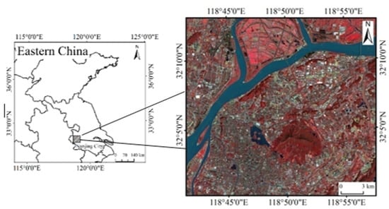
Figure 1.
Location of the study area and a Landsat 8 OLI image of the area acquired on 21 July 2017 (red, Band 4; green, Band 3; blue, Band 2).
Multitemporal cloud-free Landsat 8 satellite imageries were used in the study area in the four seasons of the same year. The acquisition dates of the Landsat 8 OLI sensor were 15 March (Spring) 2017, 21 July (Summer) 2017, 9 October (Autumn) 2017, and 12 December (Winter) 2017. Firstly, the satellite images were geometrically and radiometrically corrected. The Landsat 8 dataset has two thermal infrared (TIR) bands (Bands 10 and 11). However, due to the larger calibration uncertainty associated with TIR Band 11, it is recommended that users should work with TIR Band 10 data as a single spectral band and should not attempt a split-window algorithm using both TIR Bands 10 and 11 (https://www.usgs.gov/core-science-systems/nli/landsat/using-usgs-landsat-level-1-data-product; access on 24 March 2021). A geographic database for Nanjing city was also used for this study.
A high-resolution Chinese GF-1 image was used as the reference data for accuracy assessments. The GF-1 multispectral image (acquired on 24 July 2017) with 8 m spatial resolution was used to assess the accuracy of urban land cover derived from Landsat 8 data. The surface reflectances recorded by Landsat were retrieved from the top-of-atmosphere radiances through Fast Line-of-sight Atmospheric Analysis of Spectral Hypercubes (FLAASH) atmospheric correction. The NDVI was calculated based on the surface reflectance of Bands 4 and 5 of the Landsat 8 OLI image. The GF-1 image was used to extract land cover types to analyze the accuracy of fractional cover extracted from the Landsat data.
3. Methods
3.1. Retrieval of LST
The radiative transfer equation (RTE) was used to retrieve the LST from the Landsat thermal infrared band. Firstly, the thermal infrared band was converted to top-of-atmosphere (TOA) radiance through radiometric calibration. The second step was to remove the effects of atmospheric influence on the thermal infrared band of the Landsat data. The surface-leaving radiance LT is calculated via Equation (1) [39]:
where Lμ, Ld and τ, respectively, are the upwelling radiance, downwelling radiance, and transmission through the atmosphere. The atmospheric correction tool MODTRAN 4.1 (available at http://atmcorr.gsfc.nasa.gov/; access on 24 March 2021) was used to estimate the values of Lμ, Ld, and τ. ε is the surface emissivity calculated based on the methods of Sobrino et al. [40] and Van De Grienzd and Owe [41]. In Equation (1), Lλ is the TOA radiance image for the thermal infrared band. Because the use of thermal infrared Band 11 of Landsat TIRS is not recommended to derive LST (http://landsat.usgs.gov/Landsat8_Using_Product.php; access on 24 March 2021), the data for single spectral Band 10 of Landsat TIRS were used to retrieve the LST in this study, as for the LST retrieval of Landsat TM/ETM+.
LT = (Lλ − Lμ− τ (1− ε) Ld)/τ ε
Finally, the LST was calculated based on an inversion of Planck’s formula [42]:
LST = k2/ln[k1/LT] + 1]
In Equation (2), LST is the temperature in Kelvin (K), while k1 and k2 are the pre-launch calibration constants. For TIRS Band 10, k1 = 774.89 W/(m2srμm) and k2 = 1321.08 K.
Figure 2 shows the four seasons’ LST maps of the study area obtained from the Landsat 8 data for 2017. In Figure 2, the LST patterns of the study area obviously vary among the different seasons; the LST and UHI in summer are obviously higher than those of other seasons.
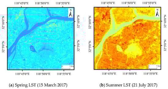
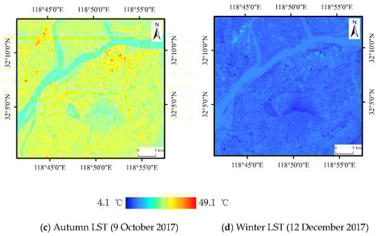
Figure 2.
The land surface temperature (LST) retrieved from the four seasons’ Landsat 8 data; spring, summer, autumn, and winter images were acquired on 15 March, 21 July, 9 October, and 12 December 2017, respectively.
3.2. Linear Spectral Unmixing by Fully Constrained Least Squares and Accuracy Assessment
Linear spectral unmixing by fully constrained least squares (FCLS) was used to extract subpixel fractional covers from the Landsat imagery in this study. All linear spectral unmixing procedures were undertaken in ENVI 4.5. The spectral unmixing procedure mainly consists of two steps: endmember extraction and fractional cover estimation. There are a variety of methods used to extract endmembers from images [14,43]. The urban environment can be assumed to consist of four fundamental components: water, vegetation, impervious surfaces, and soil. In this study, endmembers were extracted by constructing two-dimensional spectral mixing spaces. Before spectral unmixing, the water surfaces were masked out from the images because the spectral features of water are similar to those of low-albedo impervious areas. The spectrum of ISA varies widely, and impervious surfaces can be extracted by high- and low-albedo endmembers [44]; four endmembers—vegetation, high-albedo impervious surfaces (bright ISA such as concrete), low-albedo impervious surfaces (dark ISA such as asphalt), and soil—were defined. The FCLS model was used to spectrally unmix the signatures by constrained least squares, and four fractional images were derived. The high- and low-albedo percent ISA images were aggregated to form a total percent ISA image. The fraction images for ISA and vegetation in the four seasons were generated as shown in Figure 3. A multispectral GF-1 image with high spatial resolution of 8 meters was used to assess the accuracy of spectral unmixing by comparing fractional covers derived from Landsat 8 OLI data by FCLS with those from the high-resolution image. The four sampled plots used to assess the accuracy are shown in Figure 3a.
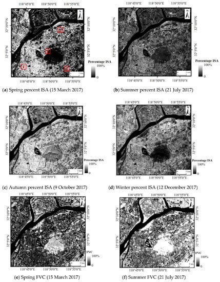
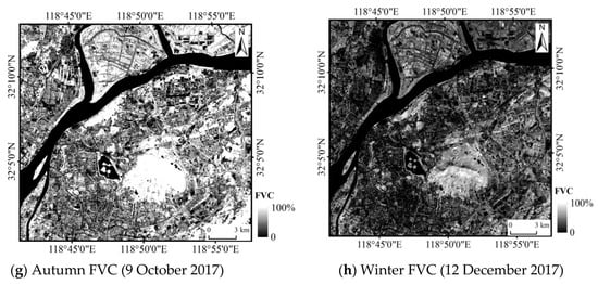
Figure 3.
Fractional cover images of impervious surface areas and vegetation derived by FCLS in the four seasons of 2017. The four sample plots in (a) were selected for accuracy assessment.
In order to assess the accuracy of the fractional cover images of ISA and vegetation derived by FCLS, we compared the fraction estimates in the sample areas with the reference data derived from the high-resolution GF-1 image. The maximum likelihood classification algorithm was used to classify the ISA and vegetation classes in the GF-1 data, and the sample areas were selected as reference data. The four sample areas in Figure 3a representing the whole study area were selected to analyze the accuracy. In this study, we only assessed the accuracy of the fractional covers derived from the Landsat data acquired in spring because the acquisition date of the high-resolution image (acquired on 2 March 2017) was close to the acquisition date of the Landsat 8 data (acquired on 15 March 2017). This approach was applicable because their acquisition dates are very close, so the land cover/vegetation phenology hardly changed between the acquisition dates of the high-resolution data and the spring Landsat 8 data.
The overall classification accuracy in the four sample plots was very similar, with less than 7% difference between the fractional covers of ISA and vegetation derived from Landsat and high-resolution data (Table 1). This accuracy can also represent the accuracy of fractional covers derived for the other three seasons. Considering the heterogeneity of the urban landscape pattern, the results indicated good agreement for ISA and vegetation cover between the areas obtained from Landsat and high-resolution data. Therefore, our method to derive fractional cover is reliable. We do not provide accuracy assessments for the other three seasons here because high-resolution images for those seasons were not available.

Table 1.
Accuracy assessment of the fractional cover of ISA and vegetation (derived by FCLS from a Landsat 8 image acquired on 15 March 2017. Areas measured in km2.
3.3. Division of the Percent ISA and Fractional Vegetation Cover
The percent ISA can indicate areas of urban development with varying development densities and patterns. Continuous percent ISA can be divided into different ISA categories to represent different levels of urban development based on equidistant ranges, and the variations of percent ISA with LST were measured to analyze the impact of variations in urban development density on the LST. In this study, each pixel with percent ISA was classified into one of four categories (0−25%, 25−50%, 50−75%, and 75−100%) representing different levels of urban development. A higher value of the percent ISA indicates higher development density/a higher level of urbanization and higher LST. Like for the classification of percent ISA, each pixel with fractional vegetation cover was also classified into one of four categories (0−25%, 25−50%, 50−75%, and 75−100% vegetation cover). A higher value of fractional vegetation cover indicates a higher cooling effect and lower LST.
By classifying the percent ISA and fractional vegetation cover into four ranges each, the urban LST in each ISA/vegetation range can be calculated, and the spatio-temporal patterns of the urban thermal environment can be analyzed and compared for the same ranges in different seasons and for different ranges (different urban development densities) in the same season.
3.4. Calculation of the Land Surface Heating Rate and Cooling Rate
Urban land cover changes from pervious to impervious surfaces increase the LST by reducing evapotranspiration and increasing sensible heat. Inversely, vegetation can decrease the LST by reducing the downward solar radiation reaching the ground and redistributing sensible heat to latent heat through evapotranspiration [45]. Different from others’ research involving regression analysis of the LST and percent ISA/FVC, in order to adapt effectively to climate change, we aimed to analyze the surface heating rate of ISA and surface cooling rate of vegetation in the urban area. In this study, the urban surface heating rate is defined as the change in LST per percentage point of percent ISA; correspondingly, the urban surface cooling rate is defined as the change in LST per percentage point of FVC. Equations (3) and (4) give, respectively, the surface heating rate (SHR) of ISA and the surface cooling rate (SCR) of vegetation.
SHR = dLST/dPI
SCR = −dLST/dFVC
In Equations (3) and (4), the LST is retrieved from remotely sensed data, PI is the percent ISA, and FVC is the fractional vegetation cover. In this study, all the LST, FVC, and LST values were derived from Landsat data. The SHR and SCR can be calculated from the slopes of linear regression between LST and percent ISA and between LST and FVC, respectively. Therefore, the SHR and SCR can be calculated based on the pixels of ISA, FVC, and LST.
Obviously, percent ISA has a positive correlation with LST, while FVC has a negative correlation with LST. The SHR and SCR reveal the heating capacity of ISA and the cooling capacity of vegetation. Through analyzing the SHR based on different ISA ranges, effects of variations in the urban different development densities on heating can be accurately assessed. As for FVC, though the relationship between LST and FVC is negative, regression analysis showed that the relationship between LST and FVC is not entirely linear [17,18]. Therefore, by analyzing the SCR based on different fractional vegetation ranges, the cooling effect of vegetation on the urban thermal environment can be more accurately assessed.
4. Results and Discussion
4.1. Variation of the LST in Different Ranges and Different Seasons
The LST varies with changes in landscape patterns and seasonal variations. As the two main urban land cover types, the composition and configuration of ISA and vegetation patches affect the spatial distribution patterns and magnitude of LST, and the LST increases with increasing percent ISA and decreases with increasing FVC. Therefore, the configuration of ISA/vegetation patches and seasonal variations influence the surface heating/cooling effects. In order to quantify the relationship between percent ISA/FVC and LST for urban climatic adaptation, we need to differentiate the influences of seasonal variations on LST based on ISA categories and FVC categories.
Urban ISA increases resulting from urban expansion can increase the LST and the intensity of UHI effects. A number of studies have used the ISA, normalized difference built-up index (NDBI), or normalized difference impervious surface index (NDISI) to analyze the ISA increase with urban expansion and its impact on the thermal environment [46,47,48]. Urban vegetation can mitigate the LST and UHI effects, and many studies have also investigated urban thermal environment change by analyzing the variations in the LST with FVC and some vegetation indices such as NDVI and EVI [7,16,22]. However, very few studies have analyzed the heating/cooling capacities (effects) of urban ISA and vegetation and their change trends in different ranges and different seasons. In order to comprehensively understand the effect of variation in ISA/vegetation on the thermal environment and to further effectively adapt to urban climate change, it is necessary to analyze the LST of different ISA/vegetation ranges and its temporal trends in different seasons firstly. Table 2 shows the mean LST values for different percent ISA ranges and FVC ranges in the study area in the four seasons of 2017. The results indicate that the LST varies in different ranges and different seasons, so we can quantify the impacts of seasonal variations on the urban LST.
Table 2.
The mean LST values for different percent ISA/FVC categories of the study area in the four seasons of 2017.
Comparing the LST in the different categories of the same season enables an analysis of the impact of an increase or decrease in ISA/vegetation resulting from urban landscape pattern change. LST increased with increasing percent ISA (from 0–25% to 75–100% percent ISA) and decreased with increasing FVC (from 0–25% to 75–100% FVC), as shown in Table 2, especially in summer. In summer, the mean LST increased nearly 4 °C from 38.3 °C at 0–25% ISA to 42.1 °C at 75–100% ISA. In winter, the mean LST only increased 0.6 °C from the low-percentage ISA category (9.8 °C at 0–25% ISA) to the highest ISA category (10.4 °C at 75–100% ISA). The increases in LST from the low-percentage ISA category to the high-percentage ISA category in spring and autumn were between those in summer and winter. In spring and autumn, the mean LST increased 1 °C and 2.1 °C, respectively, from the 0–25% ISA category to the 75–100% ISA category. Table 2 shows that the heating effects from the low-ISA category to the high-ISA category were obviously higher in summer than in other seasons. Inverse to the change trend of the LST across ISA categories in different seasons, the mean LST across the FVC categories decreased with increasing FVC from 0–25% to 75–100% FVC, and the decrease was greater in summer (lesser in winter) than in other seasons. This indicates that the cooling effect of FVC from the low-FVC category to the high-FVC category was also the highest in summer and the lowest in winter.
Table 2 indicates that the mean LST was the highest in summer, the mean LST in autumn was second highest, and the mean LST in winter was the lowest in each ISA/FVC category. By analyzing the seasonal LST difference for each category, the impact of seasonal variations on the mean LST in each category can be calculated. In addition, the impact of urban landscape pattern change on the LST can be analyzed through comparing the mean LST across different categories of the same season. Through comparing the LST based on the same or different categories in the four seasons, we can differentiate the impact of urban landscape pattern changes and seasonal variations on the thermal environment. This is important for urban planning and its adaptation to urban climatic change.
In Table 2, the mean LST for each category obviously varied among the different seasons, with especially large variation between summer and other seasons, which means that the heating/cooling effects of the ISA/FVC categories were different in different seasons. Therefore, it is necessary to further calculate and compare the SHR and SCR of the different seasons based on the percent ISA and FVC categories.
4.2. Analysis of the SHR and LST Based on Different Ranges and Different Seasons
The surface heating/cooling effects of urban surfaces are impacted by the composition and configuration of land cover types and seasonal variations (such as climatic variations, phenological characteristics of vegetation, and so on). As introduced in Section 3.4, Equations (3) and (4) of the surface heating/cooling rates indicate that the heating/cooling capacity is impacted by the LST and percentage of ISA/FVC. In order to accurately calculate the surface heating/cooling rates in this study, we calculated the surface heating/cooling rates and LST values based on the ranges of 0–25%, 25–50%, 50–75%, and 75–100% of the percent ISA and FVC for different urban development densities and compared their variations among different ranges and different seasons. This method is reasonable because the relationship between the LST and percent ISA/FVC is linear in each small range, so the heating/cooling rates and LST calculated based on each small range are more accurate than those calculated in the whole range of 0–100%.
Figure 4 presents scatter plots of the LST and percent ISA in the different seasons. The relationships between the LST and percent ISA across the whole range of 0–100% are linear in Figure 4. By visual interpretation of Figure 4, the linear relationships between the LST and percent ISA are stronger in each small range of 0–25%, 25–50%, 50–75%, and 75–100% ISA than those in the whole range of 0–100%. Therefore, the SHR and LST calculated in each small range can be more accurately analyzed and compared in different seasons than those calculated across the whole range. Based on each small range, the SHR was calculated via Equation (3) in Section 3.4 for each range in the four seasons.
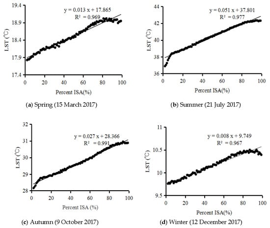
Figure 4.
Scatter plots of the LST and percent ISA in the study area in the four seasons.
In this study, our approach goes beyond an analysis of the LST and percent ISA. Here, the SHR and LST are analyzed based on each ISA category. Figure 5 shows the differences in the mean LST and SHR for the different ISA categories.
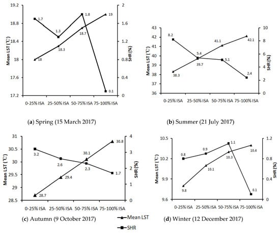
Figure 5.
The mean LST and SHR for different percent ISA categories in the four seasons.
As shown in Figure 4 and Figure 5, though the LST consistently increased with increasing percent ISA, the change trends of the SHR and percent ISA were not exactly like the change trends of the LST and percent ISA. In summer, the LST increased with increasing percent ISA, and the SHR decreased with increasing percent ISA (Figure 5b); this indicates that the increase rate of the heating capacity of ISA decreased with the percent ISA and LST increase in summer. The value of the SHR decreased from 8.2 at 0–25% ISA to 2.4 at 75–100% ISA in summer. However, the SHR varied little between the 25–50% and 50–75% ISA categories in summer (only decreased from 5.4 to 5.1), though the change trends of the LST for the two ISA categories were similar to the change trends of the LST for other ISA categories (the LST increased from 39.7 °C for the 25–50% ISA category to 41.1 °C for the 50–75% ISA category). This indicates that the increase rate of heating capacities was nearly unchanged from 25–50% to 50–75% ISA, while the LST and percent ISA increased from the 25–50% category to the 50–75% category in summer. These findings are helpful for urban planning and climatic adaption for reducing urban UHI effects. As in Equation (3) in Section 3.4, the SHR is impacted by the LST and percent ISA. Obviously, the urban LST is impacted by the composition of ISA and vegetation. Therefore, the SHR is impacted by the composition of ISA and vegetation. In Figure 5b, the value of the SHR was large at 0–25% ISA (8.2) and small at 75–100% ISA (2.4) in summer, though LST increased with increasing percent ISA. This is because the rate of increase in the LST (heating capacity) was higher in the 0–25% ISA category and decreased as the percent ISA increased (from 0–25% to 75–100% ISA) in summer. As for the 25–50% and 50–75% ISA categories, there was more vegetation present in the two categories than in the 75–100% ISA category and less vegetation than in the 0–25% ISA category in summer. The rate of LST change increased relatively little between the 25–50% and 50–75% ISA categories; therefore, the SHR was nearly unchanged across the 25–50% and 50–75% categories in summer, though LST increased with increasing percent ISA.
For autumn, the change trend of the SHR was similar to that in summer (Figure 5c). However, the value of the SHR and mean LST in autumn varied little between different ISA categories compared to those in summer. The SHR decreased from 3.2 at 0–25% ISA to 1.7 at 75–100% ISA in autumn, which meant that the heating effect changed relatively little between different ISA categories in the study area in autumn compared with summer. Compared with the SHR in summer and autumn, the SHR varied in more complex ways in spring and winter, even though the LST increased with increasing percent ISA (Figure 5a,d). The SHR was slightly higher in the 50–75% ISA category in spring and winter, which indicates that the increase rates of LST and the heating capacity in this category were higher than those in other ISA categories. Because the climate became cool in spring and cold in winter, LST increased little with the percent ISA increase, and the range of variation of the SHR was also small across the different ISA categories, especially in winter. This indicates that the heating effects increased very little with the percent ISA increase in spring and winter, especially for the 75–100% ISA category.
For urban planning and climatic adaptation, besides analysis of the variations in the LST for different seasons and different ISA ranges, analysis of SHR differences for different seasons and different ISA ranges can be used to further explore the urban thermal environment and climate adaptation under conditions of urban expansion. Through analyzing the variation in the SHR in different ISA ranges, we can obtain the distribution of the heating capacity in different urban development density areas, and through analyzing the variation of the SHR in different seasons, we can infer the impact of seasonal variation on the heating capacity. For urban planning and climatic adaptation under the conditions of urban expansion, it is necessary to analyze the impacts of urban landscape pattern change resulting from urban expansion and seasonal variations on the heating effect. This can be achieved through our SHR analytical method herein.
4.3. Analysis of the SCR and LST Based on Different Ranges and Different Seasons
Figure 6 shows scatter plots of the LST and FVC in the different seasons. The relationships between the LST and FVC across the whole range of 0–100% are not completely linear and have a negative slope, as shown in Figure 6, especially in spring and winter. By visual interpretation of Figure 6, the relationship between LST and FVC is linear in each small range of 0–25%, 25–50%, 50–75%, and 75–100% FVC. Based on each small range, the surface cooling rate was calculated via Equation (4) in Section 3.4 for each range in the four seasons.
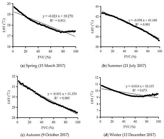
Figure 6.
Scatter plots of the LST and FVC in the study area in the four seasons.
Urban vegetation has a cooling effect on the thermal environment, especially in summer. In this study, the SCR and LST were calculated based on each FVC category, shown in Figure 7. Although the LST generally decreased as FVC increased (Figure 6 and Figure 7), the relationship between the LST and FVC was not as entirely linear in the whole range of 0–100% FVC (Figure 6) as was that between LST and percent ISA in the whole range of 0–100% percent ISA (Figure 4). Different from the decrease in SHR with increasing percent ISA in summer, the SCR increased with increasing FVC in summer (Figure 7). With increasing FVC, the SCR of vegetation increased from 3.7 in the 0–25% FVC category to 7.5 in the 75–100% FVC category in summer. This indicates that the cooling effect of vegetation increased with increasing FVC in summer, though LST decreased with increasing FVC.
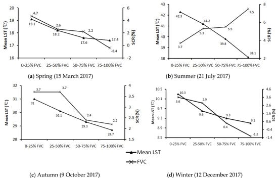
Figure 7.
The mean LST and SCR for different percent ISA categories in the four seasons.
Figure 7 shows that the cooling effect of vegetation was obviously higher in summer than in the other seasons across the different FVC categories. Different from the change trend of the SCR in summer, the SCR decreased with increasing FVC in spring, autumn, and winter. This indicates that the vegetation cooling capacity decreased with increasing FVC in spring, autumn, and winter. Because the climate of the study area is colder in spring, autumn, and winter than in summer, the cooling effects of vegetation are weaker in these colder seasons than in summer. For autumn, the range of SCR variation was the lowest among the four seasons and was unchanged between 0–25% and 25–50% FVC. As for the SCR in spring and winter, the SCR generally decreased with increasing FVC (Figure 7), indicating that the change trends of the SCR and FVC were less complicated than the change trends of the SHR and percent ISA in spring and winter (Figure 5a,d). Because the LST and FVC, to some extent, were nonlinearly correlated in the whole range of 0–100% FVC in spring and winter, and the LST slightly increased with increasing FVC at 75–100% FVC (Figure 6a,d), the values of the SCR were negative at 75–100% FVC in spring and winter (Figure 7a,d); this indicates that the LST slightly increased with increasing FVC at 75–100% FVC, and vegetation had slight heating effects in this category when the climate was cold in the study area (in spring and autumn). Figure 7 shows that the SCR variation was relatively small across the different FVC categories in spring, autumn, and winter compared to that in summer. The change trends of the SCR in different FVC ranges are helpful for urban greening and urban landscape design for UHI mitigation.
FVC is not only impacted by seasonal variation; it also has different seasonal cooling effects due to the different evapotranspiration rates in different seasons. Although the phenological characteristics of vegetation in the study area, to some extent, resulted in the variations of percent ISA and FVC derived by FCLS in the different seasons, the continuous percent ISA and FVC were divided into different categories (0–25%, 25–50%, 50–75% and 75–100% ISA/FVC categories) representing different urban landscape patterns. Therefore, the SHR and SCR calculated based on the different ISA/FVC categories can be compared among the different categories and different seasons.
Through comparing the SHR/SCR and mean LST in different ranges, we can quantify urban heating and cooling patterns and their changes under the conditions of range variations resulting from urban expansion and seasonal variations. As the analysis above shows, the heating/cooling capacities of an urban surface are impacted by the urban landscape pattern and season. An analysis of urban heating and cooling effects helps us to explore the climate adaptation potential in different development density areas of cities. This can be achieved through analyzing the surface heating and cooling rates based on different ISA and FVC categories. Different from previous studies that analyzed the relationships between percent ISA/FVC and LST, in this study we used remotely sensed data to characterize the patterns of the surface heating capacity, cooling capacity, and LST based on the urban ISA and vegetation categories; this can provide new insights into urban planning and adaptation to climate change.
5. Conclusions
Urban expansion results in landscape pattern changes of increasing ISA and decreasing vegetation cover, which increase the LST and impact the urban thermal environment. Increased temperatures due to urban expansion can result in climatic change in urban areas [49] and may have direct consequences on human health [50,51,52]. Accurate analysis of the urban landscape pattern and its impact on the thermal environment is important for mitigating the UHI effect and for urban planning.
In this paper, subpixel ISA and FVC were extracted from Landsat data by FCLS, and the accuracy was assessed by testing areas using very-high-resolution remotely sensed imagery. The subpixel fractional ISA and FVC values were further classified into four categories, and the SHR and SCR were calculated based on each ISA/vegetation category. Different from previous studies that analyzed the relationship of LST with ISA and vegetation, in this study we compared the SHR, SCR, and mean LST based on the different ranges of ISA and FVC in different seasons, and we provided a new method to explore the impact of the urban landscape pattern on the thermal environment.
The urban thermal environment is impacted by the urban landscape pattern and season. Therefore, an analysis of the SHR/SCR and mean LST in different categories and seasons can help to characterize the heating/cooling effects of ISA/vegetation and further help for urban ecological planning.
The main results of this research are as follows:
(1) In the study area, the SHR values in summer were 8.2, 5.4, 5.1, and 2.1 in the 0–25%, 25–50%, 50–75%, and 75–100% ISA categories, respectively, higher than in other seasons, and the SHR decreased with increasing LST and percent ISA in summer and autumn. When conditions were cold in spring and winter, the change trends of the SHR became more complex.
(2) The SCR increased with increasing FVC in summer and decreased with increasing FVC in spring, autumn, and winter. This indicates that the cooling capacity of vegetation increased with increasing FVC in summer and decreased with increasing FVC in other seasons. In the 75–100% FVC category, the SCR values were negative in spring (−0.4) and winter (−1.2) when the climate was cold.
(3) Seasonal variations obviously impacted the SHR, SCR, and their change trends across different ranges of ISA and vegetation cover. Compared with the SCR and FVC, the change trends of the SHR and percent ISA were generally more complicated in spring and winter.
Although the accuracy of the subpixel ISA and FVC derived from FCLS, along with the classification of the percent ISA and FVC into four ranges, impacted the results of the SHR and SCR, our methodology can integrate SHR, SCR, percent ISA, FVC, and LST to quantify the urban thermal environment and can provide information for urban planning and climate adaptation. Future research could analyze the SHR and SCR using monthly data or even day and night data based on different categories of percent ISA and FVC. In addition, it should be noted that the relationships and change trends between SHR, SCR, percent ISA, FVC, and LST may be area-dependent (the change trends may be different between different cities), and future research can further compare results for different cities under different climatic conditions.
Author Contributions
Conceptualization, Y.Z. and H.B.; methodology, Y.Z.; software, Y.L.; validation, Y.L. and Y.Z.; formal analysis, Y.Z. and Y.L.; investigation, Y.L.; resources, Y.Z.; data curation, Y.Z. and Y.L.; writing—original draft preparation, Y.Z.; writing—review and editing, H.B.; visualization, Y.L.; supervision, Y.Z.; project administration, Y.Z.; funding acquisition, Y.Z. and H.B. All authors have read and agreed to the published version of the manuscript.
Funding
This research was funded by Fujian Natural Science Foundation, China (2018J01739), and Fujian special funds for scientific research on public causes, China (2019R1002-2). H.B. was supported by the UK Natural Environment Research Council (NERC) through the National Centre for Earth Observation.
Institutional Review Board Statement
Not applicable.
Informed Consent Statement
Not applicable.
Data Availability Statement
Data available in a publicly accessible repository.
Acknowledgments
The authors would like to thank The Leicester Research Archive (LRA) for funding this work and authors would like to thank the three anonymous reviewers and editors, whose constructive criticism helped to improve the quality of the manuscript.
Conflicts of Interest
The authors declare no conflict of interest.
References
- Zhou, D.; Zhao, S.; Liu, S.; Zhang, L.; Zhu, C. Surface urban heat island in China’s 32 major cities: Spatial patterns and drivers. Remote Sens. Environ. 2014, 152, 51–61. [Google Scholar] [CrossRef]
- Berger, C.; Rosentreter, J.; Voltersen, M.; Baumgart, C.; Schmullius, C.; Hese, S. Spatio-temporal analysis of the relationship between 2D/3D urban site characteristics and land surface temperature. Remote Sens. Environ. 2017, 193, 225–243. [Google Scholar] [CrossRef]
- He, C.; Gao, B.; Huang, Q.; Ma, Q.; Dou, Y. Environmental degradation in the urban areas of China: Evidence from multi-source remote sensing data. Remote Sens. Environ. 2017, 193, 65–75. [Google Scholar] [CrossRef]
- Li, Y.; Zhang, H.; Kainz, W. Monitoring patterns of urban heat islands of the fast growing Shanghai metropolis, China: Using time-series of Landsat TM/ETM+ data. Int. J. Appl. Earth Obs. Geoinf. 2012, 19, 127–138. [Google Scholar] [CrossRef]
- Chen, Y.; Yu, S. Impacts of urban landscape patterns on urban thermal variations in Guangzhou, China. Int. J. Appl. Earth Obs. Geoinf. 2016, 54, 65–71. [Google Scholar] [CrossRef]
- Shen, H.; Huang, L.; Zhang, L.; Wu, P.; Zeng, C. Long-term and fine-scale satellite monitoring of the urban heat island effect by the fusion of multi-temporal and multi-sensor remote sensed data: A 26-year case study of the city of Wuhan in China. Remote Sens. Environ. 2016, 172, 109–125. [Google Scholar] [CrossRef]
- Zhang, Y.; Zhan, Y.; Yu, T.; Ren, X. Urban green effects on land surface temperature caused by surface characteristics: A case study of summer Beijing metropolitan region. Infrared Phys. Technol. 2017, 86, 35–43. [Google Scholar] [CrossRef]
- Zhang, Y.; Wang, X.; Balzter, H.; Qiu, B.; Cheng, J. Directional and zonal analysis of urban thermal environmental change in Fuzhou as an indicator of urban landscape transformation. Remote Sens. Environ. 2019, 11, 2810. [Google Scholar] [CrossRef]
- Voogt, J.A.; Oke, T.R. Thermal remote sensing of urban climates. Remote Sens. Environ. 2003, 86, 370–384. [Google Scholar] [CrossRef]
- Wang, C.; Wang, Z.; Wang, C.; Myint, S. Environmental cooling provided by urban trees under extreme heat and cold waves in U.S. cities. Remote Sens. Environ. 2019, 227, 28–43. [Google Scholar] [CrossRef]
- Oke, T.R. The distinction between canopy and boundary-layer heat islands. Atmosphere 1976, 14, 268–277. [Google Scholar] [CrossRef]
- Zhang, Y.; Odeh, I.; Han, C. Bi-temporal characterization of land surface temperature in relation to impervious surface area, NDVI and NDBI, using a sub-pixel image analysis. Int. J. Appl. Earth Obs. Geoinf. 2009, 11, 256–264. [Google Scholar] [CrossRef]
- Arnfield, A. Two decades of urban climate research: A review of turbulence, exchanges of energy and water, and the urban heat island. Int. J. Climat. 2003, 23, 1–26. [Google Scholar] [CrossRef]
- Weng, Q. Thermal infrared remote sensing for urban climate and environmental studies: Methods, applications, and trends. ISPRS J. Photogramm. Remote Sens. 2009, 64, 335–344. [Google Scholar] [CrossRef]
- Zhou, W.Q.; Huang, G.L.; Cadenasso, M.L. Does spatial configuration matter? Understanding the effects of land cover pattern on land surface temperature in urban landscapes. Landsc. Urban. Plan. 2011, 102, 54–63. [Google Scholar] [CrossRef]
- Zhou, W.; Wang, J.; Cadenasso, M. Effects of the spatial configuration of trees on urban heat mitigation: A comparative study. Remote Sens. Environ. 2017, 195, 1–12. [Google Scholar] [CrossRef]
- Owen, T.; Carlson, T.; Gillies, R. An assessment of satellite remotely sensed land cover parameters in quantitatively describing the climatic effect of urbanization. Int. J. Remote Sens. 1998, 19, 1663–1681. [Google Scholar] [CrossRef]
- Chen, X.; Zhao, M.; Li, P.; Yin, Z. Remote sensing image-based analysis of the relationship between urban heat island and land use/cover changes. Remote Sens. Environ. 2006, 104, 133–146. [Google Scholar] [CrossRef]
- Zhang, Y.; Harris, A.; Balzter, H. Characterizing fractional vegetation cover and land surface temperature based on sub-pixel fractional impervious surfaces from Landsat TM/ETM+. Int. J. Remote Sens. 2015, 36, 4213–4232. [Google Scholar] [CrossRef]
- Kato, S.; Yamaguchi, Y. Analysis of urban heat-island effect using ASTER and ETM+ data: Separation of anthropogenic heat discharge and natural heat radiation from sensible heat flux. Remote Sens. Environ. 2005, 99, 44–54. [Google Scholar] [CrossRef]
- Nowak, D.; Crane, D.; Stevens, J. Air pollution removal by urban trees and shrubs in the United States. Urban For. Urban. Green. 2006, 4, 115–123. [Google Scholar] [CrossRef]
- Yao, R.; Wang, L.; Gui, X.; Zheng, Y.; Zhang, H.; Huang, X. Urbanization effects on vegetation and surface urban heat islands in China’s Yangtze river basin. Remote Sens. 2017, 9, 540. [Google Scholar] [CrossRef]
- Streutker, D.R. A remote sensing study of the urban heat island of Houston Texas. Int. J. Remote Sens. 2002, 23, 2595–2608. [Google Scholar] [CrossRef]
- Wang, Z.H.; Bou-Zeid, E.; Smith, J.A. A coupled energy transport and hydrological model for urban canopies evaluated using a wireless sensor network. Q. J. R. Meteorol. Soc. 2013, 139, 1643–1657. [Google Scholar] [CrossRef]
- Howells, M.; Hermann, S.; Welsch, M.; Bazilian, M.; Segerstrom, R.; Alfstad, T.; Gielen, D.; Rogner, H.; Fischer, G.; Velthuizen, H.; et al. Integrated analysis of climate change, land use, energy and water strategies. Nat. Clim. Chang. 2013, 3, 621–626. [Google Scholar] [CrossRef]
- Bowler, D.; Buyung-Ali, L.; Knight, T.; Pullin, A. Urban greening to cool towns and cities: A systematic review of the empirical evidence. Landsc. Urban Plan. 2010, 97, 147–155. [Google Scholar] [CrossRef]
- Santamouris, M. Cooling the cities—A review of reflective and green roof mitigation technologies to fight heat island and improve comfort in urban environments. Sol. Energy 2014, 103, 682–703. [Google Scholar] [CrossRef]
- Weng, Q.; Lu, D.; Schubring, J. Estimation of land surface temperature–vegetation abundance relationship for urban heat island studies. Remote Sens. Environ. 2004, 89, 467–483. [Google Scholar] [CrossRef]
- Yuan, F.; Bauer, M.E. Comparison of impervious surface area and normalized difference vegetation index as indicators of surface urban heat island effects in Landsat imagery. Remote Sens. Environ. 2007, 106, 375–386. [Google Scholar] [CrossRef]
- Cai, G.; Du, M.; Xue, Y. Monitoring of urban heat island effect in Beijing combining ASTER and TM data. Intern. J. Remote Sens. 2011, 32, 1213–1232. [Google Scholar] [CrossRef]
- Li, J.; Wang, X.; Wang, X.; Ma, W.; Zhang, H. Remote sensing evaluation of urban heat island and its spatial pattern of the Shanghai metropolitan area, China. Ecol. Complex. 2009, 6, 413–420. [Google Scholar] [CrossRef]
- Li, J.; Song, C.; Cao, L.; Zhu, F.; Meng, X.; Wu, J. Impacts of landscape structure on surface urban heat islands: A case study of Shanghai, China. Remote Sens. Environ. 2011, 115, 3249–3263. [Google Scholar] [CrossRef]
- Xian, G.; Crane, M. An analysis of urban thermal characteristics and associated land cover in Tampa Bay and Las Vegas using Landsat satellite data. Remote Sens. Environ. 2006, 104, 147–156. [Google Scholar] [CrossRef]
- Zhang, Y.; Balzter, H.; Zou, C.; Xu, H.; Tang, F. Characterizing bi-temporal patterns of land surface temperature using landscape metrics based on sub-pixel classifications from Landsat TM/ETM+. Int. J. Appl. Earth Obs. Geoinf. 2015, 42, 87–96. [Google Scholar] [CrossRef]
- Wang, C.; Wang, Z.; Yang, J. Cooling effect of urban trees on the built environment of contiguous United States. Earth’s Future 2018, 6, 1066–1081. [Google Scholar] [CrossRef]
- Zhang, Y.; Balzter, H.; Liu, B.; Chen, J. Analyzing the Impacts of Urbanization and Seasonal Variation on Land Surface Temperature Based on Subpixel Fractional Covers Using Landsat Images. IEEE J. Sel. Top. Appl. Earth Obs. Remote Sens. 2017, 10, 1344–1356. [Google Scholar] [CrossRef]
- Nanjing Statistical Bureau. Nanjing Statistical Yearbook; Nanjing Statistical Bureau: Nanjing, China, 2018.
- Deng, S.; Katoh, M.; Guan, Q.; Yin, N.; Li, M. Interpretation of forest resources at the individual tree level at purple mountain, Nanjing city, China, using WorldvView-2 imagery by combining GPS, RS and GIS technologies. Remote Sens. 2014, 6, 87–110. [Google Scholar] [CrossRef]
- Xu, H.; Wei, Y.; Liu, C.; Li, X.; Fang, H. A scheme for the long-term monitoring of impervious−relevant land disturbances using high frequency Landsat archives and the Google Earth engine. Remote Sens. 2019, 11, 1891. [Google Scholar] [CrossRef]
- Barsi, J.; Schott, J.; Palluconi, F.; Hook, S. Validation of a web-based atmospheric correction tool for single thermal band instruments. In Earth Observing Systems X; Butler, J.J., Ed.; SPIE: Bellingham, WA, USA, 2005; Volume 5882. [Google Scholar]
- Sobrino, J.; Raissouni, N.; Li, Z. A comparative study of land surface emissivity retrieval from NOAA data. Remote Sens. Environ. 2001, 75, 256–266. [Google Scholar] [CrossRef]
- Van De Grienzd, A.; Owe, M. On the relationship between thermal emissivity and the normalized difference vegetation index for natural surfaces. Int. J. Remote Sens. 1993, 14, 1119–1131. [Google Scholar] [CrossRef]
- Chander, G.; Markham, B. Revised Landsat-5 TM radiometric calibration procedures and post calibration dynamic ranges. IEEE Trans. Geosci. Remote Sens. 2003, 41, 2674–2677. [Google Scholar] [CrossRef]
- Boardman, J.; Kruse, F.; Green, R. Mapping target signatures via partial unmixing of AVIRIS data. In Proceedings of the Summaries of the 5th Annual JPL Airborne Geoscience Workshop, Pasadena, CA, USA, 23–26 January 1995; Jet Propulsion Laboratory Publications: Pasadena, CA, USA, 1995. [Google Scholar]
- Wu, C.; Murray, A. Estimating impervious surface distribution by spectral mixture analysis. Remote Sens. Environ. 2003, 84, 493–505. [Google Scholar] [CrossRef]
- Zhang, Y.; Odeh, I.; Ramadan, E. Assessment of land surface temperature in relation to landscape metrics and fractional vegetation cover in an urban/peri-urban region using Landsat data. Int. J. Remote Sens. 2013, 34, 168–189. [Google Scholar] [CrossRef]
- Xu, H. Analysis of impervious surface and its impact on urban heat environment using the Normalized Difference Impervious Surface Index (NDISI). Photogramm. Eng. Remote Sens. 2010, 76, 557–565. [Google Scholar] [CrossRef]
- Deng, C.; Wu, C. Examining the impacts of urban biophysical compositions on surface urban heat island: A spectral unmixing and thermal mixing approach. Remote Sens. Environ. 2013, 131, 262–274. [Google Scholar] [CrossRef]
- Mussea, M.; Baronab, D.; Rodriguezc, L. Urban environmental quality assessment using remote sensing and census data. Int. J. Appl. Earth Obs. Geoinf. 2018, 71, 95–108. [Google Scholar] [CrossRef]
- Schneider, A.; Friedl, M.; Potere, D. Mapping urban areas globally using MODIS 500m data: New methods and datasets based on urban ecoregions. Remote Sens. Environ. 2010, 114, 1733–1746. [Google Scholar] [CrossRef]
- Akbari, H.; Pomerantz, M.; Taha, H. Cool surfaces and shade trees to reduce energy use and improve air quality in urban areas. Sol. Energy 2001, 70, 295–310. [Google Scholar] [CrossRef]
- Lafortezza, R.; Carrus, G.; Sanesi, G.; Davies, C. Benefits and well-being perceived by people visiting green spaces in periods of heat stress. Urban For. Urban Green. 2009, 8, 97–108. [Google Scholar] [CrossRef]


Publisher’s Note: MDPI stays neutral with regard to jurisdictional claims in published maps and institutional affiliations. |
© 2021 by the authors. Licensee MDPI, Basel, Switzerland. This article is an open access article distributed under the terms and conditions of the Creative Commons Attribution (CC BY) license (http://creativecommons.org/licenses/by/4.0/).