Abstract
Low-level jet (LLJ) significantly affects the synoptic-scale hydrometeorological conditions in the South China Sea, although the impact of LLJs on the marine ecological environment is still unclear. We used multi-satellite observation data and meteorological reanalysis datasets to study the potential impact of LLJs on the marine biophysical environment over the Beibuwan Gulf (BBG) in summer during 2015–2019. In terms of the summer average, the sea surface wind vectors on LLJ days became stronger in the southwesterly direction relative to those on non-LLJ days, resulting in enhanced Ekman pumping (the maximum upwelling exceeds 10 × 10−6 m s−1) in most areas of the BBG, accompanied by stronger photosynthetically active radiation (increased by about 20 μmol m−2 s−1) and less precipitation (decreased by about 3 mm day−1). These LLJ-induced hydrometeorological changes led to an increase of about 0.3 °C in the nearshore sea surface temperature and an increase of 0.1–0.5 mg m−3 (decrease of 0.1–0.3 mg m−3) in the chlorophyll-a (chl-a) concentrations in nearshore (offshore) regions. Intraseasonal and diurnal changes in the incidence and intensity of LLJs potentially resulted in changes in the biophysical ocean environment in nearshore regions on intraseasonal and semi-diurnal timescales. The semi-diurnal peak and amplitude of chl-a concentrations on LLJ days increased with respect to those on non-LLJ days. Relative to the southern BBG, LLJ events exhibit greater impacts on the northern BBG, causing increases of the semi-diurnal peak and amplitude with 1.5 mg m−3 and 0.7 mg m−3, respectively. This work provides scientific evidence for understanding the potential mechanism of synoptic-scale changes in the marine ecological environment in marginal seas with frequent LLJ days.
1. Introduction
More than half the world’s population now lives in coastal areas. The water quality and, as a consequence, the marine ecosystems of coastal and continental shelf waters are affected by both natural changes and human activity [1]. Continental shelves are regions of high productivity and account for about 14% of the total production of the global ocean [2]. This is due to the rapid conversion of nutrients and the high nutrient supply from rivers, wind-driven coastal upwelling, and tidal mixing [3,4,5,6,7,8]. The biophysical responses of continental shelves are affected by their width, depth, coastline, and the shape of their connection with the adjacent ocean [9,10,11], in addition to the latitude, intensity of sun exposure and seasonal temperature differences [12,13,14], and the influence of differences in the wind fields [4,15,16]. Studying the impact of changes in hydrometeorological conditions (e.g., sunshine, precipitation, temperature, and wind fields) on the marine ecological environment is therefore important in both the formation of the ecological environment and its monitoring, prediction and evaluation.
Beibuwan Gulf (BBG) is a typical continental shelf sea. It is located in the northwestern region (17–22°N, 105–110°E) of the South China Sea (SCS) and is the fourth largest fishing ground in China [17]. The BBG is a semi-enclosed gulf with complex ocean dynamics and a water depth generally <100 m. It is connected to the main SCS through the Qiongzhou Strait and an opening in the south. The BBG is therefore affected by both the SCS and the outflow from coastal rivers. A significant amount of river water flows into the BBG every year, mainly from the Red River in Vietnam and the Changhua River in Hainan, China. The Red River alone accounts for 75% of the total river runoff. The discharge of this large amount of freshwater and a rich supply of nutrients affects the temperature, salinity, ocean circulation, and phytoplankton growth of the BBG [18,19,20]. The geographical location of the BBG means that it is also affected by tides [16,21,22]. Tidal waves enter the gulf from the south and have an important impact on the circulation that drives the waters in the gulf [23].
Previous studies showed that the chlorophyll-a (chl-a) concentration and the sea surface temperature (SST) are two key indicators of the response of the upper ocean to atmospheric forcing and are required for an understanding of the hydrology, primary productivity, and water quality of this sea [24,25,26]. We aimed to obtain an in-depth understanding of the biophysical environment of the BBG and air–sea interactions in this region through the changes in chl-a concentration in the upper ocean and the SST. Ecological research in the BBG began in the 1960s. The development of satellite technology and space-borne platforms has allowed the acquisition of large-scale remote sensing data for the oceans [27,28]. On-site and satellite data are used to observe the interdecadal changes in chl-a concentration in the BBG or seasonal changes caused by the passage of the monsoon [27,28,29,30].
Except for the above influence factors (monsoon, flow outside the gulf, tidal current, etc.) that affect the marine ecosystem of the BBG, from the perspective of the weather systems, including extreme winds weather such as typhoons and low-level jets (LLJs), also affect the upper ocean. There were extensive studies of the strong impact of typhoons on the upper ocean [31,32,33,34]. On average, five typhoons pass near Hainan Island every year [35]. When a typhoon passes, it may cause phytoplankton blooms throughout the gulf [16]. LLJs usually appear below 600 hPa, with large shears in the horizontal and vertical wind speeds, which are ≥12 m s−1. LLJ are strong, narrow airflow bands with a concentrated horizontal momentum. LLJs can cause strong winds and can transport sufficient water vapor to cause strong convective weather events [36,37]. LLJs are closely related to the occurrence of heavy rain [38,39,40] and can also regulate changes in the atmospheric environment [41,42]. LLJs often occur on the coasts of the BBG in summer [40], causing windy weather and the transport of jets of water vapor in the boundary layer, which have a remarkable effect on the local weather, especially precipitation [37,40]. However, it is as yet unknown whether these strong low-level winds affect the dynamic processes of the upper ocean and change the marine environment. There has been little research on the synoptic-scale impact of LLJs on the upper marine ecological environment.
We used multi-satellite remote sensing data and meteorological reanalysis datasets to explore the temporal and spatial distribution of the chl-a concentration in the BBG (104–112°E, 15–23°N) on LLJs and non-LLJs days in summer and the potential driving factors. Section 2 introduces the satellites and reanalysis datasets and the methods used to determine the occurrence of LLJs. Section 3 shows the spatial differences in the temporal and spatial distribution of the chl-a concentration, SST and hydrometeorological elements between LLJs and non-LLJs days and their potential causes. Section 4 discusses our findings about the impact of LLJs on the synoptic scale. Section 5 summarizes our main conclusions.
2. Materials and Methods
2.1. Multi-Satellite Datasets
Both the chl-a concentration and photosynthetically active radiation (PAR) were obtained from the level 3 products of the Himawari-8 geostationary meteorological satellite launched by Japan in October 2014. The Advanced Himawari Imager onboard the Himawari-8 satellite can scan the whole Asia–Pacific region within 10 minutes. The satellite has been available for business applications since July 2015 and the time spans of the data in this paper are July–August 2015 and June–August 2016–2019. The use of geostationary satellites with a high sampling frequency can weaken the influence of adverse conditions such as clouds and precipitation [43,44,45,46]. Himawari-8 products can provide products with an hourly spatial resolution of 0.02° × 0.02° [46], making hourly temporal resolution water color remote sensing a reality [46,47] and providing an effective method for studying the influence of, and daily changes in, chl-a concentrations. Corrections and validations of the Himawari-derived chl-a data are supplied in Text S1 in the Supplementary Materials. The correction results of two types of noise for the chl-a product of Himawari-8 over SCS were shown in Figure S1.
We used a daily global SST product provided by Remote Sensing Systems (RSS) with a spatial resolution of 9 × 9 km. This product combined the characteristics of microwave radiometers that can pass through clouds [48] and the high resolution of polar-orbiting satellite infrared radiometers [49]. The product was integrated with microwave and infrared optimally-interpolated (MW_IR_OI) data [50], which mainly merged SST data from the TMI, AMSR-E, AMSR-2, WindSat, GMI, which can provide improved estimates of sea-surface roughness and improved accuracy for SSTs [51], and the SST data detected in the infrared band by the MODIS-Terra, MODIS-Aqua, and VIIRS-NPP. Through optimal interpolation can overcome the influence of severe weather, such as cloud cover, and provide long-term continuous observations at a high spatial resolution.
The wind field dataset consisted of a 10-m high wind field above the sea surface provided by RSS. This system used the RSS V7 radiometer wind, QuikSCAT, and ASCAT scatterometers to measure the wind field, the moored buoy wind field and the European Centre for Medium-Range Weather Forecasts ERA Interim reanalysis wind field dataset as the background wind field, resulting in a cross-calibrated multi-platform grid vector wind. The time resolution of the sea surface wind field data used here was 6 h and the spatial resolution was 0.25° × 0.25°. The calculation of Ekman pumping is described in Text S2 of the Supplementary Materials.
Global Precipitation Measurement Mission (GPM) was equipped with the first satellite-borne Ku/Ka band dual-frequency precipitation radar system and multi-channel GPM microwave imager, which are accurate for measuring light rain. The weather radar system can detect precipitation over a wide area [52,53,54] and the GPM satellites provided global rain and snow observations in the region 60° S–60°N. We used the final product of the Integrated Multi-satellite Retrievals for GPM daily precipitation data with a spatial resolution of 0.1° × 0.1°. This product is publicly available from the National Aeronautics and Space Administration’s Precipitation Processing System since March 2014.
2.2. Identification of LLJs
There are a number of different definitions of LLJs, although those given by Bonner [55] and Whiteman et al. [56] are widely accepted by the research community. These definitions state that LLJs only exist when the maximum wind speed occurs in the pressure layer below 700 hPa and there is a large vertical shear near the maximum wind speed layer. We used the ERA5 hourly reanalysis data for pressure levels with a spatial resolution of 0.25° × 0.25° provided by the Copernicus Climate Change Service (C3S) Climate Data Store. For an LLJ, each spatial data point needs to meet the following two requirements: (1) the maximum wind speed below 700 hPa is ≥12 m s−1 and (2) the difference between the minimum and maximum wind speeds above the layer with the maximum wind speed, but lower than 700 hPa, is ≥6 m s−1. An LLJ day is defined as when an LLJ occurs in >25% of the grid points in a certain area within 1 h and for more than 6 h (not required to be continuous) in a day, as according to Du et al. [40].
Figure 1 shows the identified LLJ days, non-LLJ days, and typhoon-affected days. We removed the typhoon days that affected the BBG in June–August and in the summer from 2015 to 2019 because typhoons bring strong winds and continue to affect the upper marine environment for at least one week after passing through an area. The identification of typhoon impact days can be referred to in Text S3 and Table S1 in the Supplementary Materials. We analyzed the LLJs days in the region of high occurrence of LLJs in the BBG (shown by the black boxes in Figure 2b and Figure 3b). The total number of days on which typhoons affected this region was 109 days if we assume that they affected the region for three to one week after passing through. The sample size was 320 days after the removal of typhoons, among which LLJs were identified on 131 days.
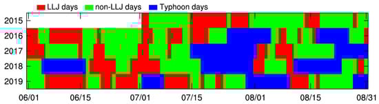
Figure 1.
Sequence of daily changes on low-level jet (LLJ) days, non-LLJ days, and days characterized by the passage of a typhoon.
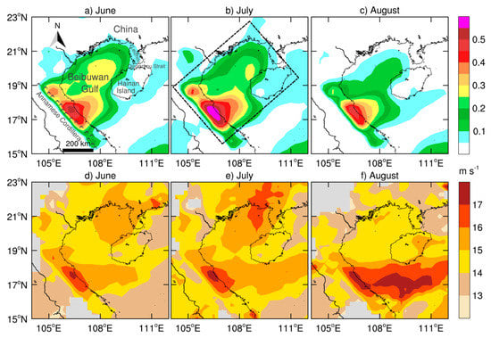
Figure 2.
Horizontal distribution of the occurrence rate of LLJs in (a) June, (b) July, and (c) August and the maximum wind speed of LLJs in (d) June, (e) July, and (f) August averaged from 2015 to 2019 over the Beibuwan Gulf (BBG), South China Sea.
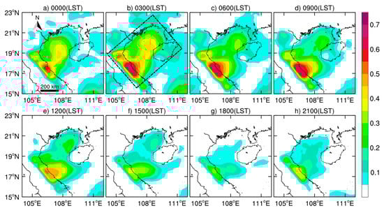
Figure 3.
Hourly horizontal distribution of the occurrence rate of LLJs (shading) over the BBG in summer from 2015 to 2019 at: (a) 0000, (b) 0300, (c) 0600, (d) 0900, (e) 1200, (f) 1500, (g) 1800, and (h) 2100 h local standard time (LST).
2.3. Difference Significance Test
We calculated the average distribution of chl-a concentrations and hydrometeorological elements for LLJ and non-LLJ days and also the difference between LLJ and non-LLJ days of these variables. A variance test method was used to test the significance at the 0.1 confidence level.
3. Results
3.1. Spatiotemporal Variation of Summer LLJs over the BBG
Figure 2 shows the monthly average spatial distribution of the LLJ occurrence rate and the maximum wind speed when LLJs occurred in the BBG during summer from 2015 to 2019. There was a clear boundary for LLJs in the southwest of the BBG and the areas of high occurrence are parallel to the coast. This was because the BBG is affected by the northwest–southeast-trending Annamese Cordillera (16–19°N, 104–108°E) and by winds over the upstream continent [57]. LLJs frequently occur along the coast of Vietnam and on the west side of Hainan Island. LLJs were most likely to occur in the BBG in July when the pressure gradient was relatively strong (Figure 2b). The maximum incidence of LLJs in July exceeded 0.6. LLJs occurred less often in August when they had the smallest range, but their average maximum wind speed was higher. The zone of maximum wind speed (>17 m s−1) was consistent with the area with a high frequency of LLJs. However, maximum wind speeds were also seen in a large area on the south side of Hainan Island in August. This area is connected to the open sea, which restricted the occurrence of LLJs.
Figure 3 and Figure S2 show the daily change in the LLJ occurrence rate [local standard time (LST) UTC + 8]. LLJs were most active at midnight and were relatively inactive in the afternoon. The zone with a high occurrence of LLJs along the Annamese Cordillera began to appear from 1800 h LST when LLJs were the least active, with an average regional incidence of only 0.054 (Figure S2). The LLJs gradually developed and there was a higher incidence >0.5 between 0000 and 0900 h LST. This was because the wind over the upstream continent was stronger at night than during the day. At sunrise, the strong turbulent mixing caused by solar radiation mainly caused low-level winds, whereas the suppression of turbulence in the mixed layer after sunset increased the wind speed [57]. Figure 3a–d show that the zone with a higher occurrence of LLJs gradually expanded to the northeast. There was also a clear area with a high incidence of LLJs in the northern BBG. The incidence of LLJs in the northern BBG reached 0.4 at 0000 h LST and this high incidence continued until 0900 h LST.
The incidence of LLJs in the central BBG reached a maximum between 0000 and 0300 h LST. The regional average diurnal frequency of occurrence also showed a similar pattern of change, decreasing during the day and gradually increasing at around 2100 h LST, reaching a maximum of 0.23 at 0500 h LST. The intensity of the LLJs changed after 2100 h LST with the same frequency as the incidence of LLJs. By contrast, the maximum change in wind speed from 0900 to 1800 h LST was the opposite of the occurrence rate and showed increased fluctuations. The wind speed at night was stronger than during the day.
3.2. Biophysical Differences between LLJs and Non-LLJs Days in Coastal Regions
LLJs affect the upper ocean through strong winds and precipitation. We analyzed the biophysical environment of the upper ocean in the BBG in summer. Figure S3 shows the average spatial distribution of the chl-a concentration, SST, wind field, and wind-driven Ekman pumping in the summer during the time period 2015–2019. In summer, the heat capacity of the land was less than that of seawater, which led to faster temperature changes on land. The river water therefore had a higher temperature than seawater. The maximum sea temperature (>30 °C) occurred on the west coast and the western mouth of the Qiongzhou Strait (Figure S3b). This may be due to the discharge of the Red River, the westerly flow of the Qiongzhou Strait, and because the three sides of the northern BBG are adjacent to the land and the shallow sea heats up quickly [20]. The SST in the central BBG was about 30 °C, whereas the SST on the southern and western coasts of Hainan Island was lower (~29 °C).
Previous studies found upwelling near the southwest coast of Hainan Island [58,59,60,61], where the SST is relatively low. This upwelling is the result of two opposing features—wind-driven downwelling (Figure S3c) and mixed tidal upwelling [59]—although the upwelling caused by tides has the major role. The dilution of seawater by water flowing from the Changhua River in summer contributes to upwelling [20]. The strong flow of water from the Changhua River coupled with the topography of the coastal area makes it easy for river water to flow into the BBG and to bring cold water up from the lower ocean. The injection of nutrients from river runoff and upwelling leads to a higher chl-a concentration on the west coast of Hainan Island (Figure S3a).
There was also a zone with a higher chl-a concentration to the west of Leizhou Peninsula and the west coast of Hainan Island. The Qiongzhou Strait and the east and west coasts of the Leizhou Peninsula have strong tidal currents [62], which agitate the nutrient-rich water in the lower layer and increased the chl-a concentrations. Regions with a high chl-a concentration were also found along the west coast of the BBG, although Hu et al. [62] reported only weak tidal currents along the coast of Vietnam based on tidal models. Even if these weak tidal currents are located in shallow coastal areas, they are too weak to stimulate the bottom eutrophic waters. The most likely sources of nutrients are therefore from rivers along the BBG (such as the Red River in the northwest) and wind-driven upwelling (Figure S3c).
Figure 4 shows the spatial distribution of the average chl-a concentration on LLJ days (Figure 4a–d), non-LLJ days (Figure 4e–h), and the difference between these two weather patterns (Figure 4i–l) from June to August and over the summer months to analyze the differences in the biophysical marine environment between LLJ days and non-LLJ days. The spatial distribution of chl-a concentration averaged by LLJ and non-LLJ days was similar with summer average pattern (Figure 4a–h and Figure S3a). In the northern part of the BBG, high chl-a concentration of above 2 mg m−3 mainly located in the coastal areas of the semi-enclosed bay, while it decreased in the offshore areas. Over time, the areas with a high chl-a concentration (>0.3 mg m−3) gradually expanded in June, July, and August. Comparing Figure 4a–h, it was found that the high-concentration belt (>2 mg m−3) near the coast was narrower on non-LLJ days than on LLJ days. However, the area of the chl-a concentration of 0.3–2 mg m−3 was larger on non-LLJ days than on LLJ days. The chl-a concentration in the central BBG on LLJ days was lower than that on non-LLJ days (Figure 4i–l) and there were many differences in the nearshore areas. The distribution of the differences was similar in June and July. The chl-a concentration decreased in the southern BBG (south of 19° N), and it decreased the most in June, with a decrease of about 0.1–0.3 mg m−3. The chl-a concentration in the northern BBG increased significantly, especially in July, with a maximum increase >0.5 mg m−3. The results for both August and summer showed an increase in nearshore areas that were more pronounced in August.
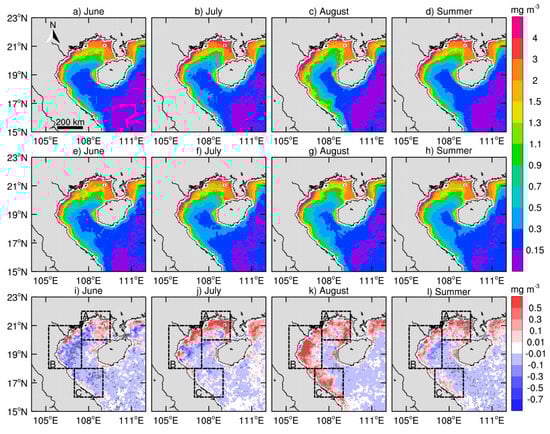
Figure 4.
Average distribution of chl-a concentrations on LLJ days in (a) June, (b) July, (c) August, and (d) summer, on non-LLJ days in (e) June, (f) July, (g) August, and (h) summer and the difference between LLJ and non-LLJ days in (i) June, (j) July, (k) August, and (l) summer (the gray dots cover areas with significant differences).
Figure 5 shows the spatial distribution of the average SST on LLJ days (Figure 5a–d), non-LLJ days (Figure 5e–h), and the differences (Figure 5i–l) from June to August and over the summer months. The average SST was similar on LLJ and non-LLJ days. In detail, the SST of the BBG in June was overall higher and the average SST of LLJ days was >31 °C (Figure 5a). In July, the seawater of the northern BBG was the warmest (>30 °C), especially on the west coast of the Leizhou Peninsula. But the SST was lowest on the east coast of the Leizhou Peninsula, the minimum SST was about 28 °C. There was a low sea temperatures band from 17°N along the coast of Vietnam to 18°N along the coast of Hainan Island (Figure 5b,f). The most obvious feature in August was that the SST on the west coast of Hainan Island was <30 °C, indicating that upwelling was strongest at this time and there was more seawater upwelling from the lower layer, making the sea surface colder. The sea temperature in the northeastern BBG on LLJ days in June was about 0.1–0.3 °C lower than that on non-LLJ days, whereas it was higher at about 0.1–0.5 °C in other sea areas (Figure 5i). This distribution was the opposite to that of the chl-a concentration. The changes in the average SST in July, August, and over the whole summer were similar to those of the chl-a concentration. The SST increased along the western shoreline of the BBG and the area of maximum temperature increase in August coincided with the area where the chl-a concentration increased. Different degrees of cooling occurred along the east coast.
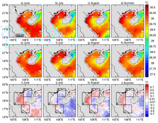
Figure 5.
Same as Figure 4 but for the sea surface temperature (SST).
There were different characteristics in every month in the northern, western, and southern coastal areas of the BBG and the reasons for the distribution of the chl-a concentration and SST in these areas may be different. We therefore divided the coastal area into three different regions to analyze the local conditions that led to the difference between LLJ and non-LLJ days: region A (northern); region B (mid-western); and region C (southern).
3.3. Potential Drivers of LLJs
Our analysis of the spatial distribution of chl-a concentrations and the SST showed that they were different in different months and therefore we determined whether the dominant factors were also different in different months. We analyzed the monthly averages of the wind field and wind-driven Ekman pumping (Figure 6), PAR (Figure 7), and precipitation (Figure 8) on LLJ and non-LLJ days and the differences between them to determine the underlying driving factors. Because the low-level wind speed was high when the LLJs appeared, it produced stronger Ekman pumping. The strong southwesterly wind in the western BBG caused stronger upwelling, whereas there was stronger downwelling (Figure 6a–d,i–l) in the eastern (west of Hainan Island) and southern (near 17°N) BBG.
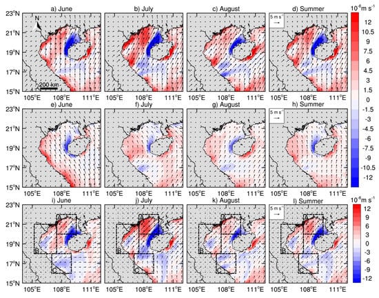
Figure 6.
Same as Figure 4 but for the wind field at 10 m (arrows) and the Ekman pumping velocity (shading; positive values represent upwelling).
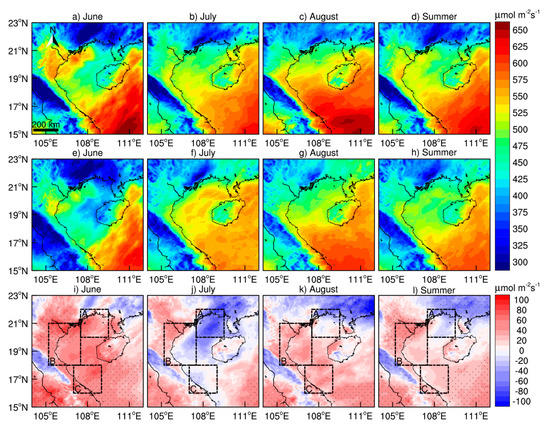
Figure 7.
Same as Figure 4 but for photosynthetically active radiation (PAR).
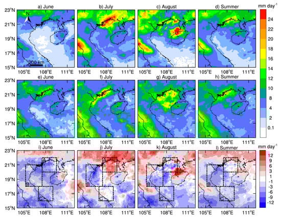
Figure 8.
Same as Figure 4 but for rainfall.
Southwesterly winds prevailed throughout the BBG in summer, but the wind field on non-LLJ days was different. The southwesterly wind had not yet developed in June and the BBG was mainly controlled by southeasterly winds, causing upwelling along the coast of Vietnam (Figure 6e). The southwesterly wind started to build up in July in the southern BBG, leading to downwelling along the coast. The wind direction then gradually changed to a southeasterly wind in the north (Figure 6f). Southwesterly winds controlled the entire BBG in August (Figure 6g). This indirectly showed that the LLJs in the BBG in summer were dominated by southwesterly winds. There were large changes in the areas with large differences in the wind direction in the northern BBG, especially in July, with the transition in the southwesterly wind on LLJ days and the southeasterly wind on non-LLJ days, leading to the largest difference in wind-driven Ekman pumping. The LLJs caused stronger upwelling in the northwest, exceeding 9 × 10⁻⁶ m s−1, and stronger downwelling on the west side of the Leizhou Peninsula and Hainan Island (less than −9 × 10⁻⁶ m s−1). Except for the northern region, where there was upwelling, most of the other areas of the gulf experienced downwelling on LLJ days. The wind field distribution in summer was the same as that in July.
Figure 7 and Figure 8 show that the spatial distributions of the PAR and precipitation. The monthly and summer spatial distribution of the PAR shows that it was high in the sea area of the BBG, whereas the surrounding land had frequent cloud and rain convective activity and a low PAR value. The PAR value of the sea area gradually extending from the gulf to the open sea was higher because the weather conditions over the open sea were relatively good, with mostly clear weather. Precipitation showed the opposite distribution to the PAR values, with the sea areas with a high PAR value having less precipitation and vice versa, and the spatial distribution was different in different months. For example, in June, when LLJs occurred in the northwestern BBG and its coastal land areas, the PAR value was >550 μmol m−2 s−1 (Figure 7a), but the precipitation was <2 mm day−1 (Figure 8a), whereas when no LLJ occurred, the PAR value in the northeastern BBG and its coastal land area was <425 μmol m−2 s−1 (Figure 7e) and precipitation was 8–10 mm day−1 (Figure 8e). The difference between the two weather conditions in the BBG in June shows that the PAR (Figure 7i) was generally about 50 μmol m−2 s−1 higher on LLJ days than on non-LLJ days, whereas precipitation was 6 mm day−1 less (Figure 8i). In July, the PAR values of the BBG and the northeastern coastal land were much lower on LLJ days (Figure 7j), but the precipitation was higher on the northern and coastal lands and lower in the western BBG (Figure 8j). In August, the PAR value in the northern BBG and its coastal land was low during LLJs (Figure 7k) and this change was close to the average summer difference (Figure 7l); precipitation showed the opposite pattern.
In the Annamese Cordillera, the PAR value on LLJ days was always lower than that on non-LLJ days. Figure 8i–l show that the precipitation on LLJ days in this area was always higher than that on non-LLJ days. During LLJs, the strong southwesterly wind blows toward the Annamese Cordillera and the warm and humid air flow is uplifted by the topography, causing clouds and rain. The PAR value in this area was therefore low and precipitation was relatively high.
These results showed that the wind speed was relatively high when LLJs appeared and therefore strong Ekman pumping was produced on days when LLJs were prevalent and the strong upwelling in the northern BBG favored an increase in the chl-a concentration. The difference in the chl-a concentration generally corresponded to the spatial distribution of the maximum wind speed (Figure 2) and upwelling (Figure 6) over most regions of BBG. Although the high incidence of LLJs was marked south of about 17°N, the chl-a concentration was suppressed as a result of downwelling, especially in June, July, and the summer. The increase in the SST near 19° N was caused by weakening of the river inflow and upwelling. The lower precipitation here is not conducive to transportation from land sources, except in August, when the chl-a concentration decreased. The distribution of the PAR was the opposite of the spatial distribution of the precipitation, but was consistent with the distribution of the SST. The SST was higher when the PAR was high in most sea areas. The reasons for the abnormal characteristics of the chl-a concentration and SST were not the same in different regions and different months. We calculated the difference between the monthly regional average LLJ and non-LLJ days in summer based on the three abnormally changing regions of the chl-a concentration and the SST (Figure 9).
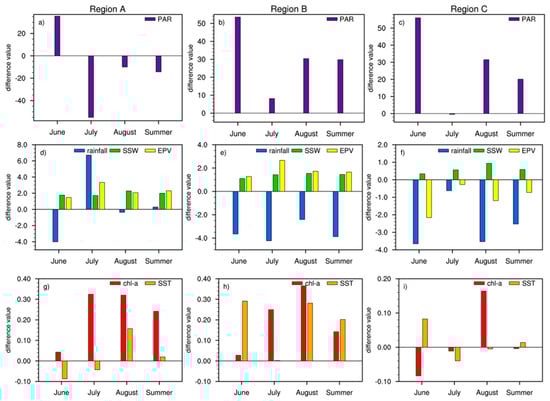
Figure 9.
Differences in hydrometeorological variables between LLJ and non-LLJ days in June, July, August, and summer in regions A, B, and C (shown by the black boxes in Figure 4i). PAR in (a) region A, (b) region B, and (c) region C. Rainfall, wind speed (SSW) and Ekman pumping (EPV) in (d) region A, (e) region B, and (f) region C. Chl-a and SST in (g) region A, (h) region B, and (i) region C.
In June, the chl-a concentration increased slightly (<0.05 mg m−3) in regions A and B on LLJ days. Less precipitation led to a decrease in terrestrial inputs, but the wind speed was higher and there was stronger upwelling. More sunlight promotes photosynthesis and leads to the growth of phytoplankton. The SST is more affected by the PAR. The SST in region A decreased due to upwelling, but there was also a large amount of upwelling in region B where the SST increased. This is because the PAR value of region B increased by 53.55 μmol m−2 s−1, the amount of radiation also increased and the sea surface became warmer. However, the decrease in the chl-a concentration in region C can be explained by the greater number of LLJ days than non-LLJ days. LLJ days are nutrient-limited, resulting in low chl-a concentrations. The surface temperature increased due to the high PAR value.
There was a lot of rain when LLJs appeared in region A in July. This excessive precipitation increased the input of nutrients to the shelf. The strong winds brought by LLJs produced upwelling, the lower layer was cold and nutrient-rich seawater surged upward. The strong upwelling in region B (>2.0 × 10⁻⁶ m s−1) resulted in an increase in the chl-a concentration. The hydrometeorological elements of LLJs in region C do not favor the growth of phytoplankton and the joint effect reduced the chl-a concentration.
The chl-a concentration of the three regions showed a high increase in August. Although the PAR value in region A was low, the wind speed was high and the rainfall relatively low, resulting in high evaporation during LLJs and heating of the sea surface, with upwelling providing nutrients for phytoplankton growth. Compared with region A, region B had more clear skies and therefore less rainfall, with an increase in the SST and stronger photosynthesis of phytoplankton leading to an increased chl-a concentration >0.35 mg m−3. The wind speed in region C was strong, but was mainly controlled by downwelling. There was less rainfall and strong sunlight, so the increase in chl-a was related to the increased amount of sunshine.
The changes in the chl-a concentration in the three regions throughout the summer were significantly positively correlated with the wind-driven upwelling. The difference in the chl-a concentration was mainly controlled by upwelling or downwelling, together with other hydrometeorological elements. Due to the different months of LLJs occurrence, that is, LLJs had intraseasonal changes, therefore the regional chl-a also responded to the intraseasonal changes of the dominant factors.
4. Discussion
The locations of the three selected nearshore regions are different, so the incidence and intensity of the LLJs may be different. Figure S4 shows the daily changes in the incidence and intensity (maximum wind speed) of LLJs in the three regions in summer. The 0800–1800 h LST in region A gradually decreased and reached the lowest value at 1800 h LST, then gradually increased and began to rise rapidly at 2200 h LST. The change trend of region B was most similar to the changing trend of the overall BBG (Figure S2), whereas the change trend in region C lagged behind. The decrease began at 1000 h LST and the frequency was highest at 0400 h LST, and then fluctuated to maintain a high incidence until 1000 h LST, with incidence rate decrease and increased process slope. The changes in intensity in regions A and B were relatively stable in the morning, reaching a secondary peak in the evening when the incidence of LLJs was the lowest. By contrast, there was no secondary peak in region C. The maximum wind speed was stable between 0800 and 1700 h LST, but the intensity decreased after 1700 h LST and started to develop rapidly at 2000 h LST.
In summer, most of the sea areas of the BBG had a high PAR value and a high SST and the chl-a concentration was lower and more uniform than in winter. As a result of the large amount of rainfall in summer and the inflow of a large amount of fresh water, the only high-value areas of chl-a concentration were in the narrow sea areas along the coast [29,63]. From the probability density distribution of the chl-a concentration in the three study areas (Figure 10) and the mean and standard deviation (Table S2), we found that the chl-a concentration in most of the seawater samples was concentrated in the low concentration range (<1.0 mg m−3). The chl-a concentration in region C was mostly concentrated in the range 0–0.5 mg m−3 (Figure 10c) and the average value in this region was about 0.1 mg m−3 lower than that in the other two regions. When the chl-a concentration was >1.0 mg m−3, the higher chl-a concentration with the lower frequency and the greater dispersion (Table S2).
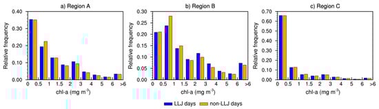
Figure 10.
Probability density distribution of chl-a concentrations on LLJ and non-LLJ days in regions (a) A, (b) B, and (c) C (shown by the black boxes in Figure 4i).
The spatial distribution of the chl-a concentration (Figure 4d,h) and the total average (Figure S3a) distribution were the same in summer and there was almost no difference in the probability density distribution of the chl-a concentration between LLJ and non-LLJ days; the changes in the mean and standard deviation were also the same. There was a particular phenomenon in region B where there were more non-LLJ days when the chl-a concentration was <1.5 mg m−3. However, when the concentration increased, the number of LLJ days also increased, which implies that the chl-a concentration was higher under the influence of LLJs. The overall probability distribution of LLJ and non-LLJ days was more consistent in region C and the influence of LLJs was small.
The semi-diurnal variation (Figure 11) and amplitude (Table 1) of the chl-a concentration in the three coastal regions were also determined. The chl-a concentration was generally higher on LLJ days than on non-LLJ days and there was a higher peak at 15:00 h LST on LLJ days, while the changes on non-LLJ days were gentler. The chl-a concentrations were high and the semi-diurnal changes were gentle in regions A and B with the same trend. By contrast, the semi-diurnal changes fluctuated significantly in region C and the chl-a concentration also increased in the evening. The amplitude of the chl-a concentration fluctuated more sharply on LLJ days and was about twice that on non-LLJ days (Table 1) in region A. The chl-a concentration in region C was low and the daily amplitude was also the lowest, although the difference between LLJ and non-LLJ days was small and the incidence of LLJ days lagged behind. This means that the high incidence rate was short in duration and the maximum wind speed had no secondary peak, which indicated that region C was less affected by LLJs. This may be because region C was located where the BBG and the open sea are connected and there are frequent exchanges of seawater. The chl-a concentration was much lower than in the other two nearshore regions (Figure 4) and was therefore less affected by LLJs than the sea area in the BBG. The diurnal variations of LLJs were not exactly the same and the different impacts of LLJs on the upper ocean in the three regions, coupled with the related hydrometeorological elements (e.g., the wind field, precipitation, PAR, and upwelling) led to differences in the biophysical environment of the upper ocean (e.g., the chl-a concentration and SST).
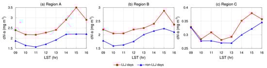
Figure 11.
Semi-diurnal variations in the chl-a concentration on LLJ and non-LLJ days in regions (a) A, (b) B, and (c) C (shown by the black boxes in Figure 4i).

Table 1.
Daily amplitude of chl-a concentrations on LLJ and non-LLJ days in regions A, B, and C (shown by the black boxes Figure 4i).
Previous studies showed that chl-a concentration in the upper BBG varies significantly and there are regional differences on seasonal and interannual scales [16,64]. Previous work focused on the impact of typhoon systems on chl-a concentrations on synoptic scales [34,65]. By contrast, our study found that synoptic-scale LLJs significantly affected the seasonal and semi-diurnal changes in the marine biophysical environment (chl-a and SST) in the BBG by modulating the changes in local hydrometeorological factors, such as the PAR, precipitation, sea surface wind vectors, and wind-driven Ekman pumping (See Figure 12). For instance, in the shores, enhanced Ekman pumping were more obviously caused by LLJs with respect to off shore (Figure 6). In addition, the precipitation on land induced by LLJ will transport more terrestrial materials to the near shore (Figure 8), which is beneficial to the increase of chl-a. Particularly, stronger PAR over nutritious nearshores (non-nutritious off shores) will induce chl-a increase (decrease) (Figure 7). These above factors synthetically led to a different spatial distribution of chl-a response to LLJ along the shores and off shores. Note that horizontal distribution of the LLJs occurrence rate and the maximum speed (Figure 2) was somewhat different from the distribution of the chl-a difference. We compared the chl-a during the LLJs days with non-LLJs days to compose chl-a differences. As mentioned above, LLJ will increase sea surface winds over most areas (Figure 6). While due to local topography with different wind direction, the Ekman pumping and precipitation with PAR were various, inducing differently regional chl-a response over BBG. The high LLJs occurrence rate and the maximum speed will not indicate obvious chl-a difference. In addition, the disturbances from oceanic internal forcing factors, such as tidal process [5,11], oceanic mesoscale eddy process [66], sea surface current, deep sea current caused by bottom topography, etc. [67,68,69], should be excluded during these intraseasonal and semi-diurnal variation processes related to LLJ events by using more in-depth observations with numerical simulation experiments. Nevertheless, our findings suggest that the potential modulation of the marine biophysical environment by synoptic-scale LLJs on multiple timescales cannot be ignored.
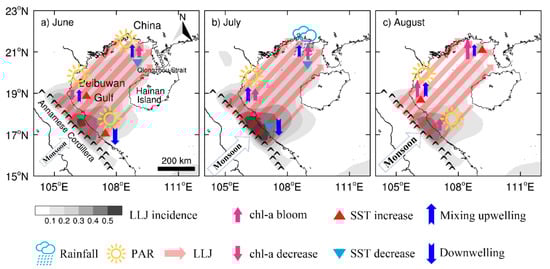
Figure 12.
The sketch map for response of hydrometeorological elements and chl-a to the LLJs in (a) June, (b) July and (c) August (shadings indicate the occurrence rate of LLJs).
5. Conclusions
We explored the temporal and spatial differences in the biophysical environment of the upper ocean of the BBG on LLJ and non-LLJ days during the summer from 2015 to 2019 using multi-source satellite remote sensing and reanalysis meteorological datasets. Our main conclusions were as follows.
LLJs were mainly caused by the southwest monsoon, the particular topography of the BBG, and the thermal difference between the land and sea surfaces. LLJs induced noticeable intraseasonal changes in the chl-a concentration and SST, especially in the nearshore areas. There were stronger southwesterly sea surface wind vectors over the BBG on LLJ days than on non-LLJ days in summer. Most sea areas, except the northern part of the BBG, had stronger PAR values, but there was less precipitation in the BBG. These factors, combined with the terrain and geographical conditions, jointly regulate the environment of the upper ocean, resulting in increases in the SST in most areas of the BBG, an increase in the chl-a concentration in the nearshore regions, and a decrease in the chl-a concentration in offshore regions.
The frequency and intensity of LLJs show intraseasonal variations, leading to similar variations in the hydrometeorological variables (e.g., the PAR, precipitation, sea surface wind vectors and wind-driven Ekman pumping) in most regions. There were clear differences in the intraseasonal change in the chl-a concentration and SST as a result of competition between these hydrometeorological factors in the three nearshore regions (northern, midwestern, and southern). The tides were weak in the northern and midwestern regions, mainly due to stronger mixing and upwelling on LLJ days, which increased the chl-a concentration. The discharge of terrigenous material related to LLJ-induced changes in the intraseasonal precipitation also affected the changes in the chl-a concentration and SST in these two nearshore regions. By contrast, the southern BBG close to the opening of the gulf was affected by downwelling and the PAR induced by LLJs—that is, the chl-a concentration decreased when LLJs caused stronger downwelling in June, whereas the chl-a concentration increased in August as a result of the strong PAR value.
The three nearshore areas showed different diurnal variations in the incidence and intensity of LLJs. This had a large influence on the semi-diurnal variation of the chl-a concentration in the gulf. The semi-diurnal peak and amplitude of the chl-a concentration on LLJ days were larger than those on non-LLJ days. Seawater exchanges were frequent in the low chl-a concentration area at the southern mouth of the gulf and the influence of LLJs on the chl-a concentration was therefore relatively weak here.
This work provides important scientific evidence to help understand the effect of LLJs on the marine ecological environment and its synoptic-scale monitoring, prediction, and evaluation. These findings will further deepen our understanding of complex multi-temporal changes in the biophysical environment of the upper ocean in marginal sea that experience frequent LLJs. Therefore, for better understanding, long-term data from Himawari-8 and GOCI-II [70] can be continuously collected in the future to simultaneously explore the interannual, intraseasonal, and semi-diurnal scales of chlorophyll-a over the South China Sea.
Supplementary Materials
The following are available online at https://www.mdpi.com/2072-4292/13/6/1194/s1, Text S1: Corrections and validations of the Himawari-derived chl-a data, Text S2: Ekman pumping, Text S3: The identification of typhoon impact days, Table S1: The typhoons impacting the Beibuwan Gulf and their impacts periods during summertime from 2015–2019, Table S2: Mean and standard deviation (std) of chl-a concentration in each segment on LLJ days and non-LLJ days in (a) Region A, (b) Region B and (c) Region C. Region A, Region B and Region C are the black boxes shown in Figure 4i, Figure S1 (a) summer chl-a concentration of Himawari-8; (b) Same as (a) but with noise removed by destriping procedure; (c) Same as (a) but with noise removed by median filter and destriping procedure., Figure S2: The hourly occurrence frequency and intensity (maximum wind speed) of LLJ over Beibuwan Gulf in summer from 2015 to 2019., Figure S3: Average spatial distribution of (a) chlorophyll-a, (b) Sea Surface Temperature and (c) wind at 10 m (arrows) and the Ekman pumping velocity (shaded, positive value is upwelling) in summer from 2015 to 2019, Figure S4: The hourly occurrence frequency and intensity (maximum wind speed) of LLJ over (a) Region A, (b) Region B and (c) Region C in summer from 2015 to 2019. Region A, Region B and Region C are the black boxes shown in Figure 4i.
Author Contributions
Conceptualization, Y.Y.; methodology, S.L. and Y.Y.; software, S.L.; validation, G.N. and Y.Y.; formal analysis, S.L., H.Y., and Y.Y.; data curation, S.L.; writing—original draft preparation, S.L.; writing—review and editing, D.T., H.Y., G.N., C.L., and Y.Y.; visualization, S.L.; supervision, Y.Y.; funding acquisition, D.T. and Y.Y. All authors have read and agreed to the published version of the manuscript.
Funding
This study was jointly supported by the NSFC-DFG (42061134009), Guangdong special support key group program (2019BT02H594), Key Special Project of Southern Marine Science and Engineering Guangdong Laboratory (Guangzhou) for Introduced Talents Team (GML2019ZD0602), Guangdong Key Laboratory of Ocean Remote Sensing (2017B030301005), Innovation Academy of South China Sea Ecology and Environmental Engineering, Chinese Academy of Sciences (ISEE2019ZR02), open funding of Guangdong Key Laboratory of Ocean Remote Sensing (2017B030301005-LORS2001), and open funding of the State Key Laboratory of Loess and Quaternary Geology (SKLLQG2010).
Institutional Review Board Statement
“Not applicable” for studies not involving human or animals.
Informed Consent Statement
“Not applicable” for studies not involving human.
Data Availability Statement
Remote Sensing Systems for the SST and wind data (http://www.remss.com/ (accessed on 28 July 2020)), Japan Aerospace Exploration Agency for the chl-a concentration and PAR product (https://www.eorc.jaxa.jp/ptree/index.html (accessed on 28 July 2020)), NASA’s Precipitation Processing System for the Integrated Multi-satellite Retrievals for GPM final precipitation product (https://pmm.nasa.gov/data-access/downloads/gpm (accessed on 28 July 2020)), and Copernicus Climate Change Service (C3S) Climate Data Store (CDS) for the ERA5 hourly data on pressure levels (https://cds.climate.copernicus.eu (accessed on 16 July 2020)).
Conflicts of Interest
The authors declare no conflict of interest.
References
- Robinson, I.S.; Antoine, D.; Darecki, M.; Gorringe, P.; Pettersson, L.; Ruddick, K.; Santoleri, R.; Siegel, H.; Vincent, P.; Wernand, M.R.; et al. Remote sensing of shelf sea ecosystems: State of the art and perspectives. J. Southeast Asian Stud. 2008, 24, 2905–2906. [Google Scholar] [CrossRef]
- Chen, C.T.A.; Liu, K.K.; Macdonald, R. Continental margin exchanges. In Ocean Biogeochemistry: The Role of the Ocean Carbon Cycle in Global Change; Global Change—The IGBP Series; Fasham, M.J.R., Ed.; Springer: Berlin/Heidelberg, Germany, 2003; pp. 53–97. [Google Scholar] [CrossRef]
- Tang, D.L.; Kawamura, H.; Doan-Nhu, H.; Takahashi, W. Remote sensing oceanography of a harmful algal bloom off the coast of southeastern Vietnam. J. Geophys. Res. Ocean 2004, 109, 325–347. [Google Scholar] [CrossRef]
- Largier, J.L.; Lawrence, C.A.; Roughan, M.; Kaplan, D.M.; Dever, E.P.; Dorman, C.E.; Kudela, R.M.; Bollens, S.M.; Wilkerson, F.P.; Dugdale, R.C.; et al. West: A northern california study of the role of wind-driven transport in the productivity of coastal plankton communities. Deep Sea Res. Part II 2006, 53, 2833–2849. [Google Scholar] [CrossRef]
- Sharples, J.; Tweddle, J.F.; Mattias Green, J.A.; Palmer, M.R.; Kim, Y.N.; Hickman, A.E.; Holligan, P.M.; Mark Moore, C.; Rippeth, T.P.; Simpson, J.H.; et al. Spring-neap modulation of internal tide mixing and vertical nitrate fluxes at a shelf edge in summer. Limnol. Oceanogr. 2007, 52, 1735–1747. [Google Scholar] [CrossRef]
- Paul, J.H.; Kedong, Y.; Lee, J.H.W.; Gan, J.P.; Liu, H.B. Physical–biological coupling in the Pearl River Estuary. Cont. Shelf Res. 2008, 28, 1405–1415. [Google Scholar] [CrossRef]
- Tang, C.H.; Wong, C.K.; Lie, A.A.Y.; Yung, Y.K. Size structure and pigment composition of phytoplankton communities in different hydrographic zones in Hong Kong’s coastal seas. J. Mar. Biol. Assoc. UK 2015, 95, 885–896. [Google Scholar] [CrossRef]
- Wu, M.L.; Hong, Y.G.; Yin, J.P.; Dong, J.D.; Wang, Y.S. Evolution of the sink and source of dissolved inorganic nitrogen with salinity as a tracer during summer in the Pearl River Estuary. Sci. Rep. 2016, 6, 36638. [Google Scholar] [CrossRef]
- Weisberg, R.H.; Black, B.D.; Li, Z. An upwelling case study on florida’s west coast. J. Geophy. Res. Ocean 2000, 105. [Google Scholar] [CrossRef]
- Longhurst, A. Ecological Geography of the Sea, 2nd ed.; Academic Press: San Diego, CA, USA, 2007; p. 542. [Google Scholar] [CrossRef]
- Schafstall, J.; Dengler, M.; Brandt, P.; Bange, H. Tidal-induced mixing and diapycnal nutrient fluxes in the mauritanian upwelling region. J. Geophys. Res. 2010, 115. [Google Scholar] [CrossRef]
- Walsh, J.J. Shelf-sea ecosystems. In Analysis of Marine Ecosystems; Longhurst, A.R., Ed.; Academic Press: London, UK, 1980; pp. 159–196. [Google Scholar] [CrossRef]
- Ward, B.A.; Waniek, J.J. Phytoplankton growth conditions during autumn and winter in the Irminger sea, North Atlantic. Mar. Ecol. Prog. Ser. 2007, 334, 47–61. [Google Scholar] [CrossRef]
- Yoder, J.A.; Schollaert, S.E.; O’Reilly, J.E. Climatological phytoplankton chlorophyll and sea surface temperature patterns in continental shelf and slope waters off the northeast U.S. coast. Limnol. Oceanogr. 2002, 47. [Google Scholar] [CrossRef]
- Botsford, L.W.; Lawrence, C.A.; Dever, E.P.; Hastings, A.; Largier, J. Effects of variable winds on biological productivity on continental shelves in coastal upwelling systems. Deep Sea Res. Part II 2006, 53, 3116–3140. [Google Scholar] [CrossRef]
- Bauer, A.; Waniek, J.J. Factors affecting chlorophyll a concentration in the central Beibu Gulf, South China Sea. Mar. Ecol. Prog. Ser. 2013, 474, 67–88. [Google Scholar] [CrossRef]
- Liu, Z.L.; Ning, X.R.; Cai, Y.M. Distribution characteristies of size-fractionated chlorophyll-a and productivity of phytoplankton in the Beibu Gulf. Acta Oceanol. Sin. 1998, 20, 50–57. [Google Scholar] [CrossRef]
- Maren, D.S.V.; Hoekstra, P. Dispersal of suspended sediments in the turbid and highly stratified red river plume. Cont. Shelf Res. 2005, 25, 503–519. [Google Scholar] [CrossRef]
- Maren, D.S.V. Water and sediment dynamics in the red river mouth and adjacent coastal zone. J. Asian Earth Sci. 2007, 29, 508–522. [Google Scholar] [CrossRef]
- Shen, C.; Yan, Y.; Zhao, H.; Pan, J.; Adam, T.D. Influence of monsoonal winds on chlorophyll-α distribution in the Beibu Gulf. PLoS ONE 2018, 13, e0191051. [Google Scholar] [CrossRef]
- Shi, M.; Chen, C.; Xu, Q.; Lin, H.; Liu, G.; Wang, H.; Wang, F.; Yan, J. The role of Qiongzhou Strait in the seasonal variation of the South China Sea circulation. J. Phys. Oceanogr. 2002, 32, 103–121. [Google Scholar] [CrossRef]
- Wu, D.; Wang, Y.; Lin, X.; Yang, J. On the mechanism of the cyclonic circulation in the Gulf of Tonkin in the summer. J. Geophys. Res. Ocean. 2008, 113, C09029. [Google Scholar] [CrossRef]
- Cai, S.; Huang, Q.; Long, X. Three-dimensional numerical model study of the residual current in the South China Sea. Oceanol. Acta 2003, 26, 597–607. [Google Scholar] [CrossRef]
- Liu, K.K.; Chao, S.Y.; Shaw, P.T.; Gong, G.C.; Chen, C.C.; Tang, T.Y. Monsoon-forced chlorophyll distribution and primary production in the South China Sea: Observations and a numerical study. Deep Sea Res. Part I 2002, 49, 1387–1412. [Google Scholar] [CrossRef]
- Yang, Y.J.; Xian, T.; Sun, L.; Fu, Y.F. Summer Monsoon Impacts on Chlorophyll-a Concentration in the Middle of the South China Sea: Climatological Mean and Annual Variability. Atmos. Ocean. Sci. Lett. 2012, 5, 15–19. [Google Scholar] [CrossRef]
- Tan, S.C.; Wang, H. The transport and deposition of dust and its impact on phytoplankton growth in the Yellow Sea. Atmos. Environ. 2014, 99, 491–499. [Google Scholar] [CrossRef]
- Hu, S.; Zhou, W.; Wang, G.; Cao, W.; Xu, Z.; Liu, H.; Wu, G.; Zhao, W. Comparison of Satellite-Derived Phytoplankton Size Classes Using In-Situ Measurements in the South China Sea. Remote Sens. 2018, 10, 526. [Google Scholar] [CrossRef]
- Cham, D.D.; Son, N.T.; Minh, N.Q.; Thanh, N.T.; Dung, T.T. An analysis of shoreline changes using combined multitemporal remote sensing and digital evaluation model. Civ. Eng. J. 2020, 6, 1–10. [Google Scholar] [CrossRef]
- Tang, D.L.; Kawamura, H.; Lee, M.A.; Dien, V.T. Seasonal and spatial distribution of chlorophyll-a concentrations and water conditions in the Gulf of Tonkin, South China Sea. Remote Sens. Environ. 2003, 85, 475–483. [Google Scholar] [CrossRef]
- Wu, Y.C.; Guo, F.; Huang, L.F.; Huang, F.P. Distribution characteristics of chlorophyll a content in the Beibu Gulf. Guangzhou Chem. Ind. 2014, 42, 144–146. (In Chinese) [Google Scholar] [CrossRef]
- Zheng, G.M.; Tang, D.L. Offshore and nearshore chlorophyll increases induced by typhoon winds and subsequent terrestrial rainwater runoff. Mar. Ecol. Prog. Ser. 2007, 333, 61–74. [Google Scholar] [CrossRef]
- Fu, D.; Pan, D.; Mao, Z.; Ding, Y.; Chen, J. The effects of chlorophyll-a and SST in the South China Sea area by typhoon near last decade. SPIE Eur. Remote Sens. 2009, 7478, 74782E. [Google Scholar] [CrossRef]
- Jiang, X.P.; Zhong, Z.; Jiang, J. Upper ocean response of the South China Sea to Typhoon Krovanh (2003). Dyn. Atmos. Ocean. 2009, 47, 165–175. [Google Scholar] [CrossRef]
- Liu, S.H.; Li, J.G.; Sun, L.; Wang, G.H.; Tan, D.L.; Huang, P.; Yan, H.; Gao, S.; Liu, C.; Gao, Z.Q.; et al. Basin-wide responses of the South China Sea environment to Super Typhoon Mangkhut (2018). Sci. Total Environ. 2020, 731, 139093. [Google Scholar] [CrossRef]
- Chen, Y.Q.; Tang, D.L. Remote sensing analysis of impact of typhoon on environment in the sea area south of Hainan Island. Procedia Environ. Sci. 2011, 10, 1621–1629. [Google Scholar] [CrossRef]
- Tollerud, E.I.; Caracena, F.; Koch, S.E.; Jamison, B.D.; Hardesty, R.M.; Mccarty, B.J.; Kiemle, C.; Collander, R.S.; Bartels, D.L.; Albers, S. Mesoscale moisture transport by the Low-Level Jet during the IHOP field experiment. Mon. Weather Rev. 2008, 136, 3781–3795. [Google Scholar] [CrossRef][Green Version]
- Berg, L.K.; Riihimaki, L.D.; Qian, Y.; Yan, H.P.; Huang, M.Y. The Low-Level Jet over the Southern Great Plains determined from observations and reanalyses and its impact on moisture transport. J. Clim. 2015, 28, 6682–6706. [Google Scholar] [CrossRef]
- Higgins, R.W.; Yao, Y.; Yarosh, E.S.; Janowiak, J.E.; Mo, K.C. Influence of the great plains Low-Level Jet on summertime precipitation and moisture transport over the Central United States. J. Clim. 1997, 10, 481–507. [Google Scholar] [CrossRef]
- Monaghan, A.J.; Rife, D.L.; Pinto, J.O.; Davis, C.A.; Hannan, J.R. Global precipitation extremes associated with diurnally varying Low-level Jets. J. Clim. 2010, 23, 5065–5084. [Google Scholar] [CrossRef]
- Du, Y.; Zhang, Q.; Chen, Y.L.; Zhao, Y.; Wang, X. Numerical simulations of spatial distributions and diurnal variations of Low-Level Jets in china during early summer. J. Clim. 2014, 27, 5747–5767. [Google Scholar] [CrossRef]
- Darby, L.S.; Allwine, K.J.; Banta, R.M. Nocturnal low-level jet in a mountain basin complex. part II: Transport and diffusion of tracer under stable conditions. J. Appl. Meteorol. Clim. 2006, 45, 740–753. [Google Scholar] [CrossRef]
- Hu, X.M.; Klein, P.M.; Xue, M.; Zhang, F.; Doughty, D.C.; Forkel, R.; Joseph, E.; Fuentes, J.D. Impact of the vertical mixing induced by Low-level Jets on boundary layer ozone concentration. Atmos. Environ. 2013, 70, 123–130. [Google Scholar] [CrossRef]
- Wang, M.; Ahn, J.; Jiang, L.; Shi, W.; Son, S.; Park, Y.; Ryu, J. Ocean color products from the Korean Geostationary Ocean Color Imager (GOCI). Opt. Express 2013, 21, 3835–3849. [Google Scholar] [CrossRef]
- Hsu, P.-C.; Lu, C.-Y.; Hsu, T.-W.; Ho, C.-R. Diurnal to Seasonal Variations in Ocean Chlorophyll and Ocean Currents in the North of Taiwan Observed by Geostationary Ocean Color Imager and Coastal Radar. Remote Sens. 2020, 12, 2853. [Google Scholar] [CrossRef]
- Liu, X.; Wang, M. Analysis of ocean diurnal variations from the Korean Geostationary Ocean Color Imager measurements using the DINEOF method. Estuar. Coast. Shelf Sci. 2016, 180, 230–241. [Google Scholar] [CrossRef]
- Murakami, H. Ocean color estimation by Himawari-8/AHI. In Proceedings of the SPIE Asia-Pacific Remote Sensing, New Delhi, India, 4–7 April 2016; Volume 9878, p. 987810. [Google Scholar] [CrossRef]
- Ryu, J.; Han, H.; Cho, S.; Park, Y.; Ahn, Y. Overview of geostationary ocean color imager (GOCI) and GOCI data processing system (GDPS). Ocean Sci. J. 2012, 47, 223–233. [Google Scholar] [CrossRef]
- Wentz, F.J.; Gentemann, C.L.; Smith, D.K.; Chelton, D. Satellite measurements of sea surface temperature through clouds. Science 2000, 288, 847–850. [Google Scholar] [CrossRef]
- Donlon, C.; Rayner, N.; Robinson, I.; Poulter, D.J.S.; Casey, K.S.; Vazquez Cuervo, J.; Armstrong, E.; Bingham, A.; Arino, O.; Gentemann, C.; et al. The Global Ocean Data Assimilation Experiment High-resolution Sea Surface Temperature Pilot Project. Bull. Am. Meteorol. Soc. 2007, 88, 1197–1213. [Google Scholar] [CrossRef]
- Gentemann, C.L.; Meissner, T.; Wentz, F.J. Accuracy of satellite sea surface temperatures at 7 and 11 GHz. IEEE Trans. Geosci. Remote Sens. 2010, 48, 1009–1018. [Google Scholar] [CrossRef]
- Reynolds, R.W.; Smith, T.M. Improved global sea surface temperature analyses using optimum interpolation. J. Clim. 1994, 7, 929–948. [Google Scholar] [CrossRef]
- Kuriqi, A. Assessment and quantification of meteorological data for implementation of weather radar in mountainous regions. Mausam 2016, 67, 789–802. [Google Scholar]
- Abdulrazzaq, Z.T.; Hasan, R.H.; Aziz, N.A. Integrated TRMM Data and Standardized Precipitation Index to Monitor the Meteorological Drought. Civ. Eng. J. 2019, 5, 1590–1598. [Google Scholar] [CrossRef]
- Yang, Y.J.; Wang, H.; Chen, F.J.; Zheng, X.Y.; Fu, Y.F.; Zhou, S.X. TRMM-based Optical and Microphysical Features of Precipitating Clouds in Summer over the Yangtze-Huaihe River Valley, China. Pure Appl. Geophys. 2019, 176, 357–370. [Google Scholar] [CrossRef]
- Bonner, W.D. Climatology of the Low-Level Jet. Mon. Weather Rev. 1968, 96, 833–850. [Google Scholar] [CrossRef]
- Whiteman, C.D.; Bian, X.; Zhong, S. Low-Level Jet Climatology from Enhanced Rawinsonde Observations at a Site in the Southern Great Plains. J. Appl. Meteorol. 1997, 36, 1363–1376. [Google Scholar] [CrossRef]
- Kong, H.; Zhang, Q.; Du, Y.; Zhang, F. Characteristics of coastal low-level jets over Beibu Gulf, China, during the early warm season. J. Geophys. Res. Atmos. 2020, 125. [Google Scholar] [CrossRef]
- Chen, Z.Z.; Hu, J.Y.; Sun, Z.Y.; Zhu, J. Sectional features of temperature and salinity in Beibu Gulf during July–August, 2006. In Marine Scientific Research Papers in Beibu Gulf, 2nd ed.; Li, Y., Hu, J.Y., Eds.; The Ocean Publishing Company: Beijing, China, 2008; pp. 85–86. (In Chinese) [Google Scholar]
- Lv, X.G.; Qiao, F.L.; Wang, G.S.; Xia, C.S.; Yuan, Y.L. Upwelling off the west coast of Hainan Island in summer: Its detection and mechanisms. Geophys. Res. Lett. 2008, 35, 196–199. [Google Scholar] [CrossRef]
- Chen, Z.H.; Qiao, F.L.; Xia, C.S.; Wang, G. The numerical investigation of seasonal variation of the cold water mass in the Beibu Gulf and its mechanisms. Acta Oceanol. Sin. 2015, 34, 44–54. [Google Scholar] [CrossRef]
- Gao, J.S.; Wu, G.D.; Ya, H.Z. Review of the circulation in the Beibu Gulf, South China Sea. Cont. Shelf Res. 2017, 138, 106–119. [Google Scholar] [CrossRef]
- Hu, J.Y.; Kawamura, H.; Tang, D. Tidal front around the Hainan Island, northwest of the South China Sea. J. Geophys. Res. Ocean 2003, 108. [Google Scholar] [CrossRef]
- Huang, Y.C.; Li, Y.; Shan, H.; Li, Y.H. Seasonal variations of sea surface temperature, chlorophyll a and turbidity in Beibu Gulf, MODIS imagery study. J. Xiamen Univ. 2008, 47, 856–863. (In Chinese) [Google Scholar]
- Wang, Y.; Yao, L.; Chen, P.; Yu, J.; Wu, Q. Environmental influence on the spatiotemporal variability of fishing grounds in the Beibu Gulf, South China Sea. J. Mar. Sci. Eng. 2020, 8, 957. [Google Scholar] [CrossRef]
- Ye, H.J.; Sui, Y.; Tang, D.L.; Afanasyev, Y.D. A subsurface chlorophyll a bloom induced by typhoon in the South China Sea. J. Mar. Syst. 2013, 128, 138–145. [Google Scholar] [CrossRef]
- Wang, G.; Chen, D.; Su, J. Generation and life cycle of the dipole in the South China Sea summer circulation. J. Geophys. Res. 2006, 111. [Google Scholar] [CrossRef]
- Xie, S.P.; Chang, C.H.; Xie, Q.; Wang, D.X. Intraseasonal variability in the summer South China Sea: Wind jet, cold filament, and recirculations. J. Geophys. Res. 2007, 112. [Google Scholar] [CrossRef]
- Wang, D.; Wang, Q.; Cai, S.; Cai, S.; Shang, X.; Peng, S.; Shu, Y.; Xiao, J.; Xie, X.H.; Zhang, Z.; et al. Advances in research of the mid-deep South China Sea circulation. Sci. China Earth Sci. 2019, 62. [Google Scholar] [CrossRef]
- Shi, W.; Huang, Z.; Hu, J. Using TPI to Map Spatial and Temporal Variations of Significant Coastal Upwelling in the Northern South China Sea. Remote Sens. 2021, 13, 1065. [Google Scholar] [CrossRef]
- Yang, H.; Han, H.J.; Heo, J.M.; Jeong, J.; Kwak, S. Ocean Color Algorithm Development Environment for High-Speed Data Processing of GOCI-II. In Proceedings of the IGARSS 2018—2018 IEEE International Geoscience and Remote Sensing Symposium, Valencia, Spain, 22–27 July 2018; pp. 7968–7971. [Google Scholar] [CrossRef]


Publisher’s Note: MDPI stays neutral with regard to jurisdictional claims in published maps and institutional affiliations. |
© 2021 by the authors. Licensee MDPI, Basel, Switzerland. This article is an open access article distributed under the terms and conditions of the Creative Commons Attribution (CC BY) license (http://creativecommons.org/licenses/by/4.0/).