GRACE-Derived Time Lag of Mekong Estuarine Freshwater Transport in the Western South China Sea Validated by Isotopic Tracer Age

Abstract

Estuarine freshwater transport has a substantial impact on the near-shore ecosystem and coastal ocean environment away from the estuary. This paper introduces two independent methods to track the Mekong freshwater-induced mass transport by calculating the time lag (or equivalently, the phase) between in situ Mekong basin runoff and the equivalent water height (EWH) time series over the western South China Sea from a gravity recovery and climate experiment (GRACE). The first method is the harmonic analysis that determines the phase difference between annual components of the two time series (called the P-method), and the other is the cross-correlation analysis that directly obtains the time lag by shifting the lagged time series forward to attain the highest cross-correlation between the two time series (called the C-method). Using a three-year rolling window, the time lag variations in three versions of GRACE between 2005 and 2012 are computed for demonstrating the consistency of the results. We found that the time lag derived from the P-method is, on average, slightly larger and more variable than that from the C-method. A comparison of our gridded time lag against the age determined via radium isotopes in September, 2007 by Chen et al. (2010) revealed that our gridded time lag results were in good agreement with most isotope-derived ages, with the largest difference less than 6 days. Among the three versions of the GRACE time series, CSR Release 05 performed the best. The lowest standard deviation of time lag was ~1.6 days, calculated by the C-method, whereas the mean difference for all the time lags from the isotope-derived ages is ~1 day by P-method. This study demonstrates the potential of monitoring Mekong estuarine freshwater transport over the western South China Sea by GRACE.

1. Introduction

The Mekong river basin is the largest tropical water resource in Southeast Asia, dominated by the annual flood pulse. Its estuary annually discharges approximately 475 km³ freshwater and 160 million tons of sediment into the South China Sea (SCS) [1]. Most heavy sediment settles down quickly along the coast, while buoyant freshwater discharged from the estuary forms a river plume that can be transported on the ocean surface hundreds of kilometers away [2]. The near-field river plume located within 300 km off the coast can be modeled under static-state balance via runoff flux, local current, wind, and ocean tides [3,4,5]. Direct field sampling, such as isotope sampling, enables us to derive the freshwater ages from the estuaries of the Amazon river [6], the Mississippi river [7], the Yangtze river [8] and the Mekong river [9] to their adjacent ocean. Partly due to the costs of field trips and reliability issues [10], it remains a challenge to monitor the continuous spatiotemporal variation in Mekong freshwater transport.

Remotely sensed ocean color yields the spatial extent of the dissolved components in surface water [11], and chlorophyll concentration enables us to track the dispersal of the Amazon river plume [12]. In the western SCS, chlorophyll data have also been well studied along with sea surface temperature, wind, height anomalies [13], and eddies [14]. However, both suspended particular matter and chlorophyll-a concentrations relevant to the Mekong river mostly appeared along the coastlines, using different bio-optical algorithms [15,16]. Though the spatial extent can be mapped, it remains difficult to calculate the time spent to get from the estuary to a particular location on the ocean surface, in particular an ocean area more than 300 km away from the estuary.

In essence, freshwater is a mode of mass transfer from the estuary to the ocean. These spatiotemporal mass variations have been continuously monitored by the gravity recovery and climate experiment (GRACE) since 2002 [17,18]. With a ~300 km spatial resolution, GRACE-derived equivalent water heights (EWHs) are employed to quantify continental and oceanic mass fluctuations [19], enabling the study of climate [20], continental hydrology and glaciology [21] and oceanography [22]. Recently, studies of coastal regions have gradually emerged with post-processing on the ocean/land boundary, including mass-derived sea surface height and ocean bottom pressure anomalies in open gulfs [23,24], and sediment accumulation and discharge for large rivers [25,26]. Note that the land-to-ocean spatial leakage error of GRACE data products is unneglectable in the ocean within 250 km of the coasts, and additional corrections should be applied [24,27], but the leakage effects are numerically shown to be negligible when the data grid points are located more than 250 km away from the coasts [28,29]. Therefore, so long as the time series of the GRACE data points is located more than 250 km away from the coastlines, it can be safely utilized for oceanic applications.

In contrast to the aforementioned oceanic applications, the usage of GRACE-derived estuarine freshwater-induced mass variations on the ocean surface remains unexplored, let alone the calculation of spatiotemporal variation of freshwater age 800 km from the estuary. This paper aims to introduce a cost-effective method using in situ runoff and satellite-derived freshwater-induced mass variations to determine the variable time lag (distinguishable from water age derived by isotope) from the Mekong river estuary to the western SCS. Two independent methods were employed to retrieve the regional time lag in the western SCS based on a three-year rolling window in order to reduce the uncertainty and ensure sufficient valid periods for data fitting simultaneously. Finally, the GRACE-derived time lags generated from the two methods are then compared to the isotope-derived age measured in September 2007 [9].

Section 2 presents our study region, three datasets (i.e., three versions of GRACE data, in situ runoff and isotope data), and their processing strategies. Two independent methods, phase analysis (P-method) and cross-correlation analysis (C-method), are introduced in Section 3. In Section 4, we present the regional averaged time lag results separately derived by the two methods in the western SCS with interpretation, followed by evaluating the gridded time lag distribution of the two methods during different time periods, and finally, we compare our satellite-derived time lag with the isotope-derived age in 2007. Section 5 summarizes our conclusion.

2. Study Area and Data Description

2.1. Mekong River Estuary and Western SCS

Originating from the Tibetan Plateau, the Mekong river is the largest river in Southeast Asia. In the southern Indochina Peninsula, the Mekong river flows through Thailand, Laos and Cambodia, followed by the Mekong river delta, where it splits into the Bassac river and the lower Mekong river, before finally discharging into the SCS (Figure 1). Driven by the southwest monsoon, the downstream area of the Mekong basin normally generates a flood pulse in summer, which contributes ~84% of the annual total river discharge [30]. During wet and dry conditions, the Tonle Sap Lake in Cambodia and dam operations also help regulate the seasonal river flux along the main stream [31,32,33].

The SCS is a western marginal sea of the Pacific ocean with significant water exchange through the Karimata, Malacca and Luzou straits [34]. Between June and September every year, the predominant northwestward along-shore current affects the tropical river plume extension [4]. Estuarine mixtures are transported to the western SCS when Mekong runoff normally peaks in September. Besides this, the well-known eastward South Vietnam upwelling at about 12°N and frequent eddies in summer further complicate the sea surface variability [35,36]. The global El Niño–Southern Oscillation (ENSO) events, which are closely associated with the interannual variability of tropical monsoons, also cause anomalous changes in both the Mekong basin runoff and oceanic dynamics in this geographic region [37,38]. As such, Mekong freshwater transport in the western SCS will be affected by the above combined effects.

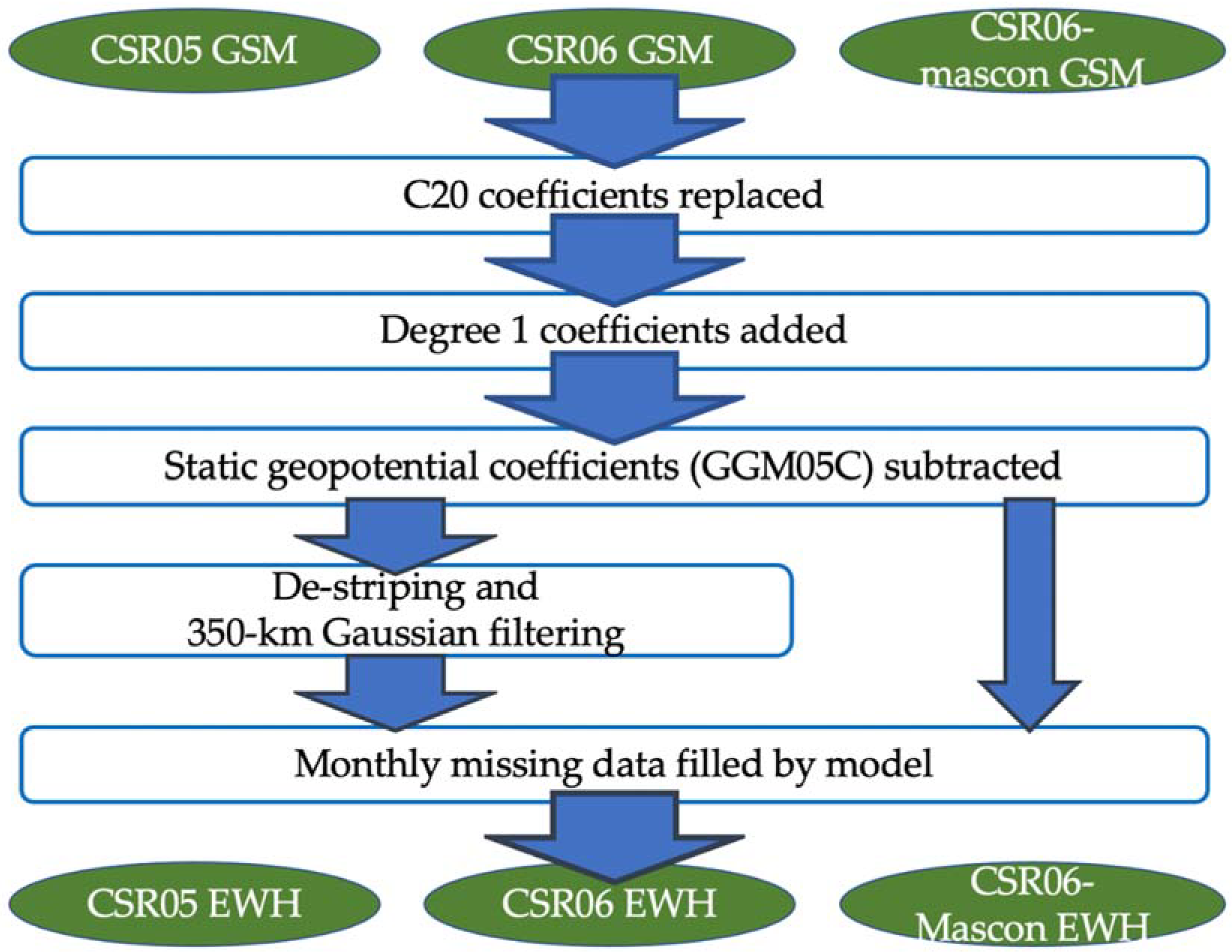
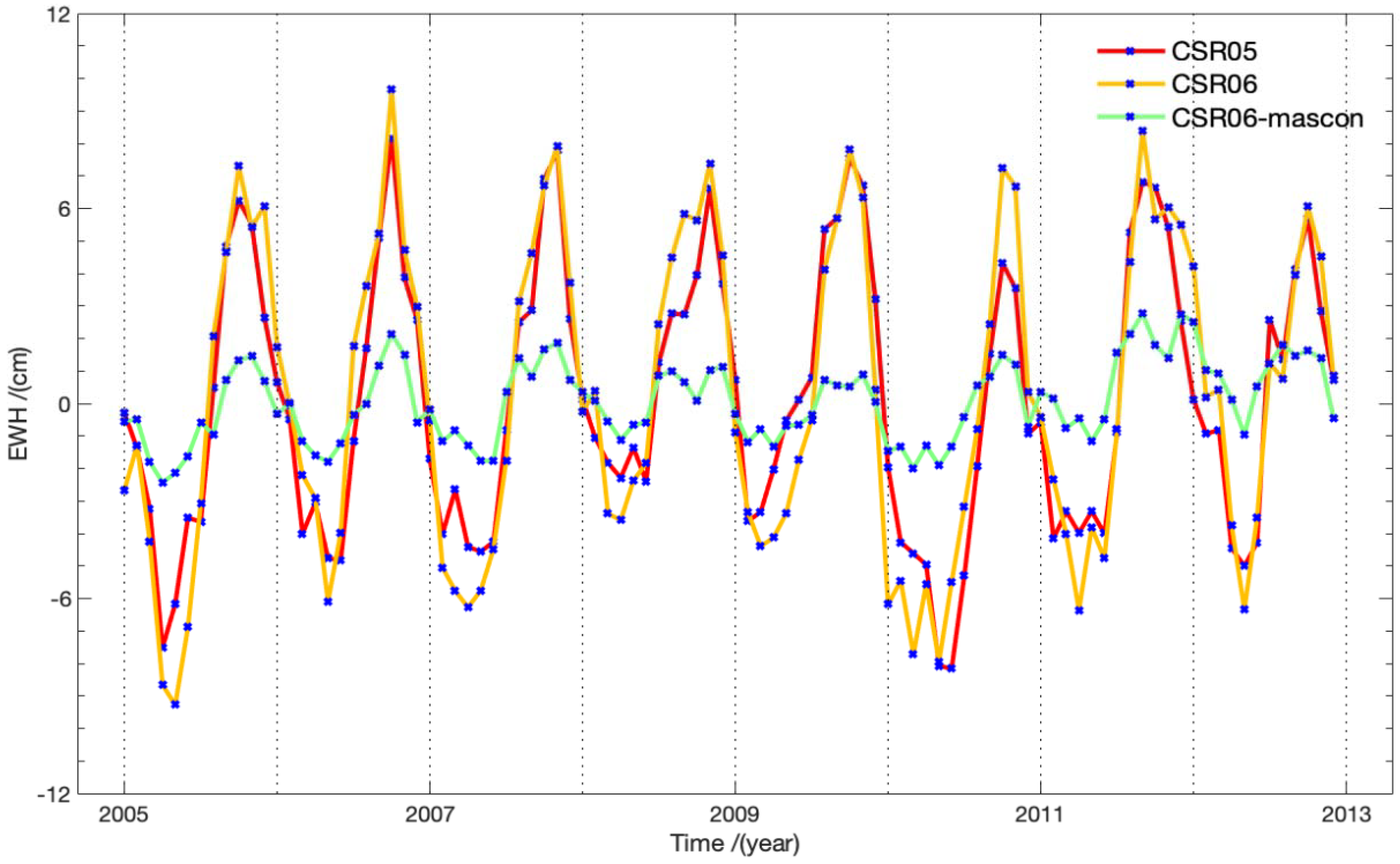
2.2. Oceanic EWH Time Series from GRACE

In this study, three versions of GRACE monthly data from the Center for Space Research at the University of Texas (CSR) were used: Level-2 Release 05 (CSR05), Level-2 Release 06 (CSR06), and a recent mascon solution based on CSR06 (CSR06-mascon). The first two versions of the relative gravity field, in the form of 60 degree and order of spherical harmonic (SH) coefficients (i.e., GSMs), were accessible at http://icgem.gfz-potsdam.de/series (accessed on 20 March 2021). The last one used the recently employed regional mass concentration functions (mascons) to parameterize the Earth’s gravity field [39]. The CSR06-mascon product with all relevant corrections in a 0.25° × 0.25°grid format could be directly used and was accessible at http://www2.csr.utexas.edu/grace/ (accessed on 20 March 2021). [40]. All data products were converted into EWH for our investigation.

Note that GSM represents geopotential coefficients after corrections to errors of commission or omission from the background gravity models [41], in which they were corrected by a priori models of solid and ocean tides, pole tides, non-tidal atmospheric and oceanic loadings, etc. Customarily, to study the oceanic mass variation, part of the non-tidal atmospheric and oceanic loading from the Atmosphere and Ocean De-Aliasing Level-1B (AOD1B)-modeled data product (i.e., the GAD component) was re-added back to the GSM in order to restore the ocean bottom pressure [42] or mass-induced sea level variation [26]. Nonetheless, the AOD1B-modeled data did not account for river flux into the ocean [43]. Therefore, to study the freshwater mass variations in the ocean surface caused by river flux in our present investigation, we directly used GSM.

The following steps (Figure 2) were employed to derive the EWH time series for GRACE Level-2 CSR05 and CSR06 data products: (1) C₂₀ coefficients were replaced with that observed via satellite laser ranging [44]; (2) geocenter motion was added to the degree-1 SH coefficient [45]; (3) the SH coefficients of the GGM05C gravity field [46] was subtracted; (4) a de-striping procedure and 350 km Gaussian filtering were applied to reduce the combined noises in the high degrees of the SH coefficients [47]. Notice that the CSR06-mascon EWH was free from step (4), because the compact geodesic grid and the design of the regularization matrix had already taken into consideration the conditions of land and ocean separately [39].

Moreover, a linear model with the offset, trend, and periodic terms was used to fill the missing monthly data. To avoid the potential seismic signal contamination before and after the nearby Sumatra–Andaman earthquake in December 2004 [48], the data spanning from 2005 to 2012 were used with missing data in January 2011, June 2011, August 2012 and October 2012, interpolated through the fitting equation (2) below. GRACE data after 2012 were not selected because at least three monthly data sets were missing for each year. All the EWHs were resampled into 1° × 1° grids. Following the above procedures, the average gridded EWH time series over 9–15°N and 110–114°E in the western SCS (blue regions in Figure 1) are presented in Figure 3. Among the three time series, the EWHs generated from CSR05 and CSR06 matched each other well, but the EWH generated from the CSR06-mascon presented a much lower amplitude (i.e., ~1.5 cm) than those from CSR05 and CSR06 (i.e., ~5 cm). This difference depends on the completely different inversion methodology used for inferring EWHs, in addition to the refined geophysical corrections.

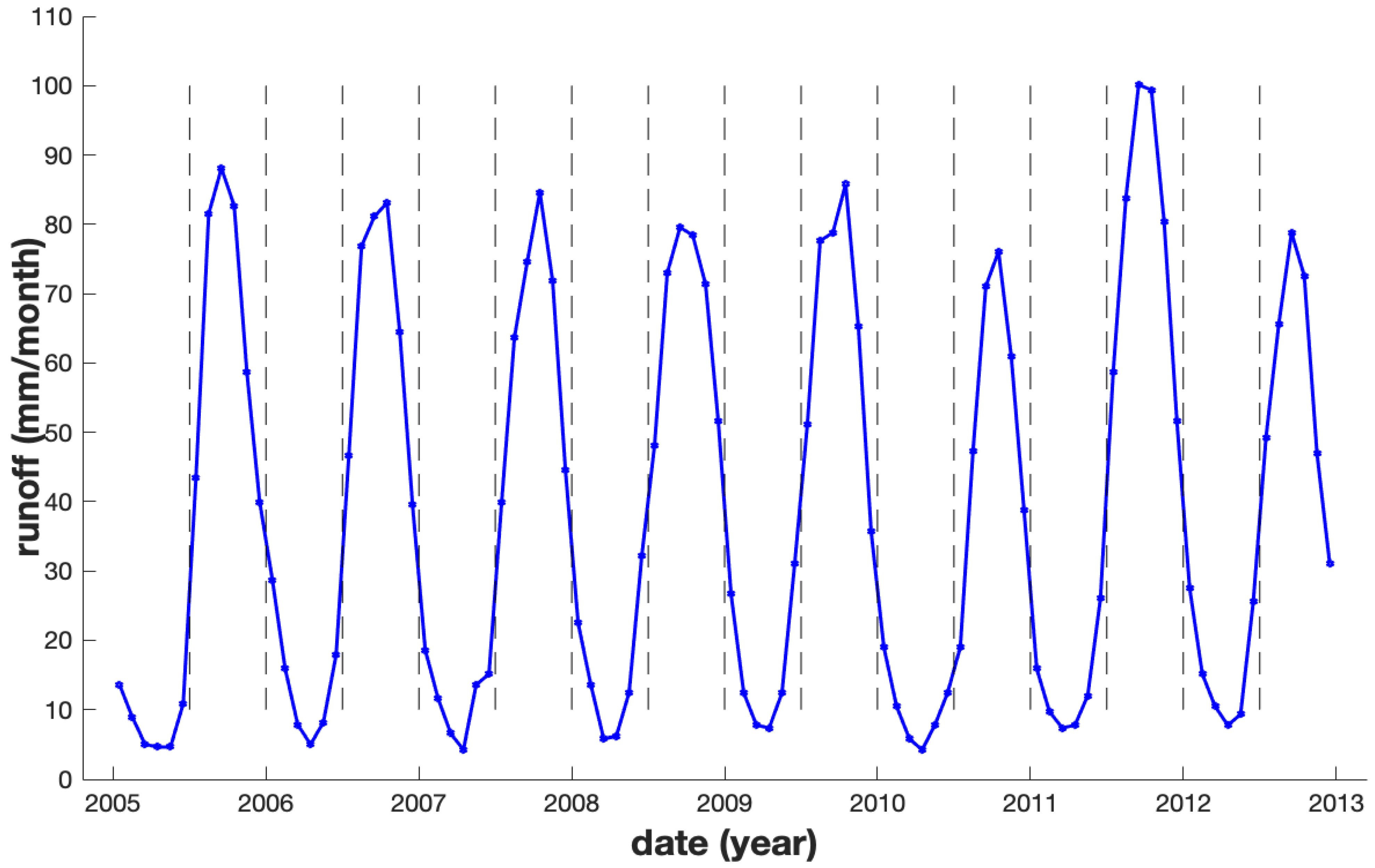
2.3. Mekong Basin Runoff from In Situ Hydrological Stations

Along the two main tributaries of the Mekong estuary mouth, the Chau Doc and Tan Chau hydrological stations are about 200–300 km away from both the inland Tonle Sap Lake and the estuary mouth (Figure 1). Therefore, the effects of lake regulation and the backwater due to ocean tides on the runoff were minimized [49]. Note that we assumed that sub-surface discharge was negligible when compared to the main flow. Then, the observed discharge time series of the two stations were summed up in order to represent the whole basin runoff and average out the ocean tidal backwater effect due to semidiurnal and diurnal ocean tides. Both in situ discharge time series can be requested from the Mekong River Commission (MRC) (http://www.mrcmekong.org accessed on 20 March 2021).

To be consistent with the GRACE data time span, the daily discharge time series spanning between January 2005 and December 2012 were selected. To convert the unit of the daily discharge (in m³/s) into runoff (mm), it was divided by the total Mekong river basin drainage area (i.e., 795,000 km²), while adding up daily values of each month. In general, the Mekong basin runoff generally reaches its maximum and minimum in September and April, respectively. During the strong La Niña event during 2010–2011, the runoff reached the lowest peak value at ~76 mm in 2010 and the highest peak value of over 100 mm in 2011 (Figure 4). Besides this, to be consistent with the GRACE EWH anomalies, runoff time series were subtracted from the mean of the entire study period.

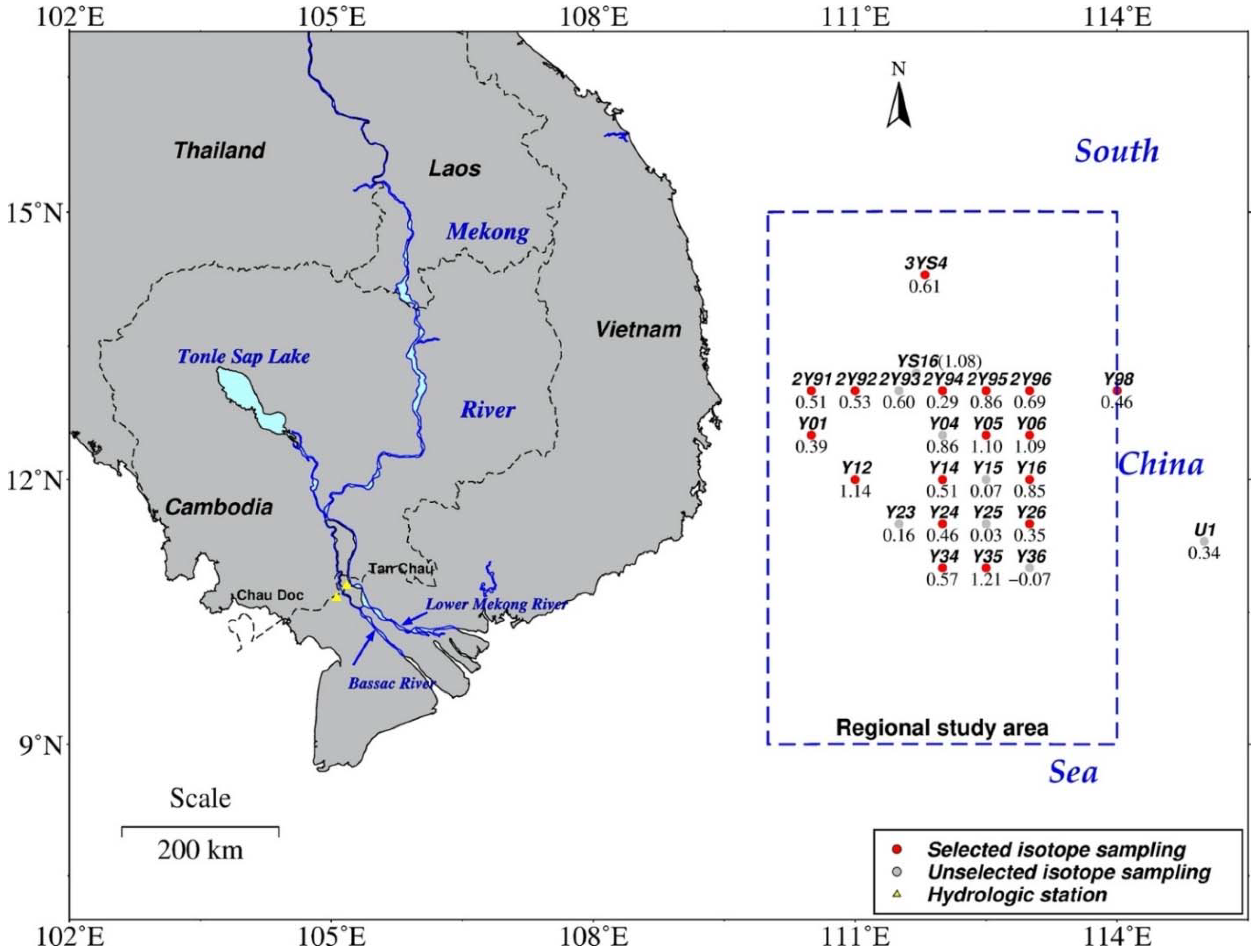
2.4. Isotope-Derived Age Based on Radium Isotope Data Measured in 2007

Ref. [9] investigated the distributions of the ²²³Ra, ²²⁶Ra, and ²²⁸Ra isotopes, and salinity variations, on the ocean surface of the western SCS during a one-month field trip between August and September 2007. Based on an empirical two-end-member mixing model [6,50], the apparent age of the Mekong river plume freshwater was determined (at dots shown in Figure 1), serving as a ground truth to validate our GRACE-derived time lag. Note that the ground truths are located more than 800 km away from estuary mouth. Hence, the land-to-ocean leakage effects of the GRACE data should be negligible. The isotope-derived apparent age (t) of each sample can be calculated by:

$$t=-\frac{\ln \left[\frac{{}_{}{}^{223}R{a}_{obs}}{{}_{}{}^{223}R{a}_{es}\times f_{es}}\right]}{{\lambda }_{223}}$$

(1)

where ${}_{}{}^{223}R{a}_{obs}$ and $f_{es}$ represent ²²³Ra activity (in disintegrations per minute (dpm)/100 L) and the dimensionless estuarine fraction of each sampling (modeled with an input of the ²²⁸Ra and ²²⁶Ra activities and salinity), respectively; ${}_{}{}^{223}R{a}_{es}$ represents the ²²³Ra activity of estuarine end-member sampling (with a default constant of 0.74 dpm/100 L), and ${\lambda }_{223}$ is the decay constant of ²²³Ra, which was 0.061 d⁻¹. The age, t, of the Mekong river plume samples is depicted in Figure 1.

Considering the high uncertainty and sensitivity resulting from the end-member coefficients in the model, extremely anomalous samplings were not chosen where (1) the contribution of the Mekong river plume to the surface water, $f_{es}$, was less than 0.2 or greater than 1.0, and (2) the calculated age was less than 0.2 months (i.e., 6 days). Under these criteria, 17 out of 25 isotope samples remained (at red dots shown in Figure 1), whose derived ages would be further compared to GRACE-derived time lags. All Mekong river plume sample positions, $f_{es}$, and ages are listed in

Table A1. The information of radium isotope sampling for the Mekong river plume group adapted with permission from ref. [9], Copyright 2010 American Geophysical Union.

Sample Code	Longitude (°E)	Latitude (°N)	fes	Age (month)
3YS4	111.8	14.3	0.83	0.61
YS16	111.7	13.2	1.47	1.08
2Y91	110.5	13.0	0.90	0.51
2Y92	111.0	13.0	0.46	0.53
2Y93	111.5	13.0	1.29	0.60
2Y94	112.0	13.0	0.46	0.29
2Y95	112.5	13.0	0.33	0.86
2Y96	113.0	13.0	0.29	0.69
Y06	113.0	12.5	0.60	1.09
Y05	112.5	12.5	0.60	1.10
Y04	112.0	12.5	1.30	0.86
Y01	110.5	12.5	0.41	0.39
Y12	111.0	12.0	0.77	1.14
Y14	112.0	12.0	0.96	0.51
Y15	112.5	12.0	0.40	0.07
Y16	113.0	12.0	0.89	0.85
Y26	113.0	11.5	0.36	0.35
Y25	112.5	11.5	0.50	0.03
Y24	112.0	11.5	0.60	0.46
Y23	111.5	11.5	0.65	0.16
Y34	112.0	11.0	0.65	0.57
Y35	112.5	11.0	0.50	1.21
Y36	113.0	11.0	0.40	−0.07
U1	115.0	11.3	0.18	0.34
Y98	114.0	13.0	0.90	0.46

, with unselected sample codes and corresponding extreme values underlined.

3. Methodology

Time lag analysis was conducted to determine the time lag between in situ runoff near the estuary mouth and the freshwater component of the GRACE EWH time series on the ocean surface in our study region. Two methods were employed. One is a harmonic analysis to determine the annual phase of in situ runoff and GRACE EWH time series, followed by taking the phase difference between them (hereinafter called the P-method); the other is performing the cross-correlation analysis via an empirical shift in GRACE EWH time series against the in situ runoff in our study region until reaching maximum cross-correlation (hereinafter called the C-method). Each method is independent of the other, except that the latter one used the detrended time series generated from the former one for calculating cross-correlation.

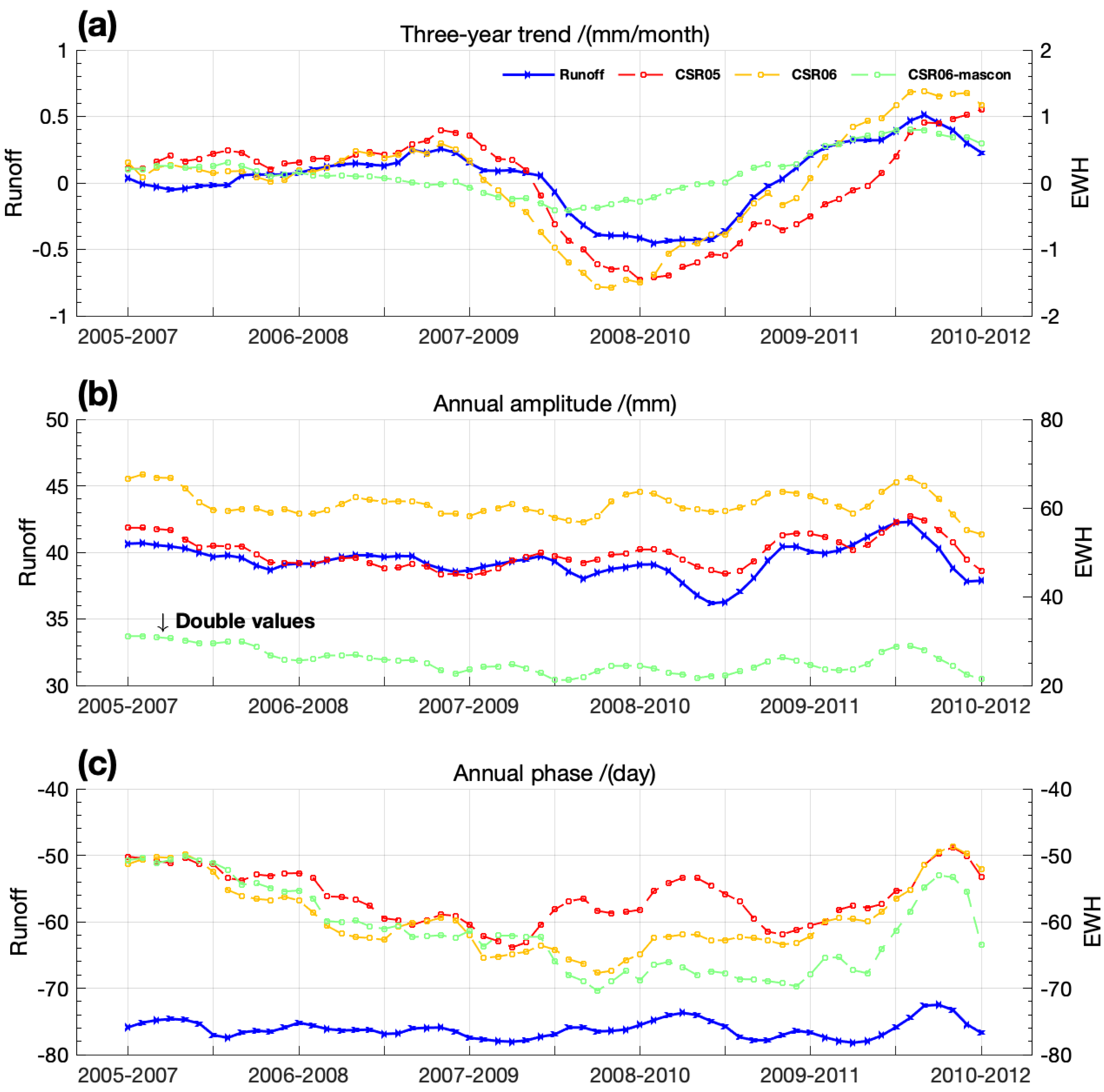
3.1. Phase Analysis (P-Method)

To obtain the phase of semi-annual and annual signals of EWH, a conventional harmonic analysis is employed, which is expressed as:

$$EWH\left(t\right)=a+bt+{\sum }_{i=1}^2{A}_i\cos \left(\frac{2\pi }{T_i}\left(t-{\phi }_i\right)\right),$$

(2)

where $a$ and $b$ are the offset and the linear trend; $A_i$ and ${\phi }_i$ represent the corresponding amplitude and phase with predefined period $T_i$ for annual ($i$ = 1) and semiannual ($i$ = 2) signals, respectively. Six parameters (i.e., a, b, $A_1$, $A_2$, ${\phi }_1$, and ${\phi }_2$) are to be determined via least-squares estimation. The same model has also been used for monthly in situ runoff and filling the missing data of monthly EWH.

According to the regional averaged result from the western SCS from 2005 to 2012 (

Table A2. Annual and semiannual amplitude and phase, long-term trend of runoff and three EWHs, from 2005 to 2012.

	Runoff	CSR05	CSR06	CSR06- Mascon
Annual amplitude (mm)	39.60	50.42	60.41	12.62
Semiannual amplitude (mm)	7.15	9.56	7.48	2.00
Annual phase (day)	−77.23	−55.31	−55.64	−58.26
Semiannual phase (day)	8.34	23.09	16.75	–19.29
Long-term trend (mm/year)	0.15	0.15	0.24	1.59

), the annual amplitude is several times larger than the semiannual one, in terms of both runoff and EWHs. Ignoring the semi-annual one, the freshwater time lag from the Mekong estuary (specifically at two hydrological stations) to our study region could be calculated as the annual phase (${\phi }_1$) difference between EWH and runoff.

Considering the variance calculated for the lower frequency, at least three complete cycles of data should be used in order to be more representative in terms of statistics [51]. We also evaluated the subsequent difference in our results by sequentially adding one more year of data span for data fitting in our study area starting from 2005 [52] (See Appendix B). We found that the difference (in terms of root-mean-square error (RMSE)) was stabilized when a three-year data time span was employed for all three GRACE time series. The RMSE converges to less than 10 mm/year (Figure A1). Therefore, a three-year data time span was adopted as a data window rolling month-by-month during 2005–2012.

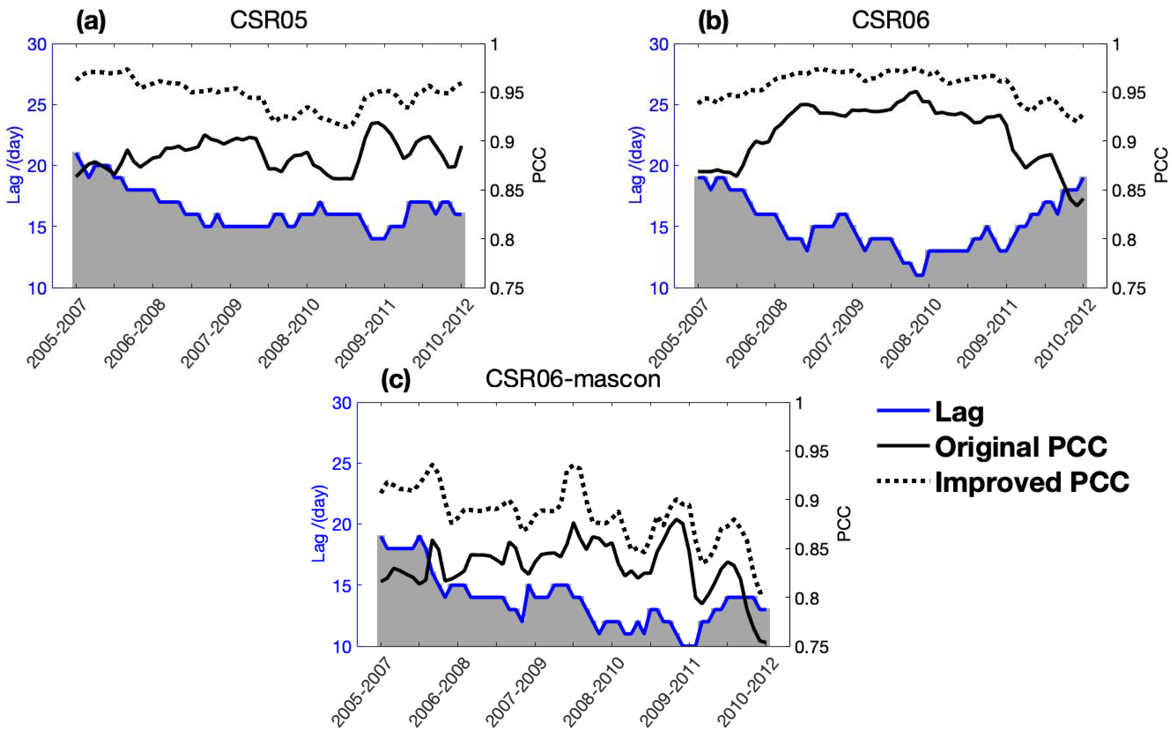
3.2. Cross-Correlation Analysis (C-Method)

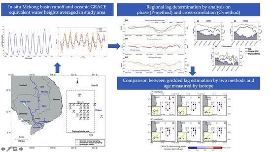
The cross-correlation between EWH and runoff time series allows us to empirically determine the spatial distribution of time lag, representing freshwater transport on the ocean surface. The cross-correlation is, in fact, a Pearson correlation coefficient (PCC) introduced with a time shift, $\delta \tau$, expressed as:

$$PCC\left(\delta \tau \right)=\frac{{\sum }_{i=1}^N\left(R^i-\overline{R}\right)\left(E^{i+\delta \tau }-\overline{E}\right)}{\sqrt{{\sum }_{i=1}^N{\left(R^i-\overline{R}\right)}^2{\sum }_{i=1}^N{\left(E^{i+\delta \tau }-\overline{E}\right)}^2}}$$

(3)

where $R^i$ and $E^{i+\delta \tau }$ are the runoff and EWHs at month $i$ and month $i+\delta \tau$, respectively, and $\overline{R}$ and $\overline{E}$ are their mean values. Finally, when the $PCC\left(\delta \tau \right)$ reaches the maximum, the corresponding $\delta \tau$ is considered as the optimal freshwater time lag.

In this method, the monthly detrended runoff and EWHs time series were interpolated to a daily interval based on a bi-cubic interpolation algorithm in MATLAB. Note that interpolation is necessary for daily $\delta \tau$ despite the fact that this process would introduce unavoidable uncertainty into our results. In addition, the cross-correlation is less dependent on the length of time series. Note that whenever time shift $\delta \tau$ is applied, the number of valid fitting months in the formula, N, is slightly less than the given time period. Therefore, the three-year rolling window method was still applied in order to be consistent with the P-method.

4. Results

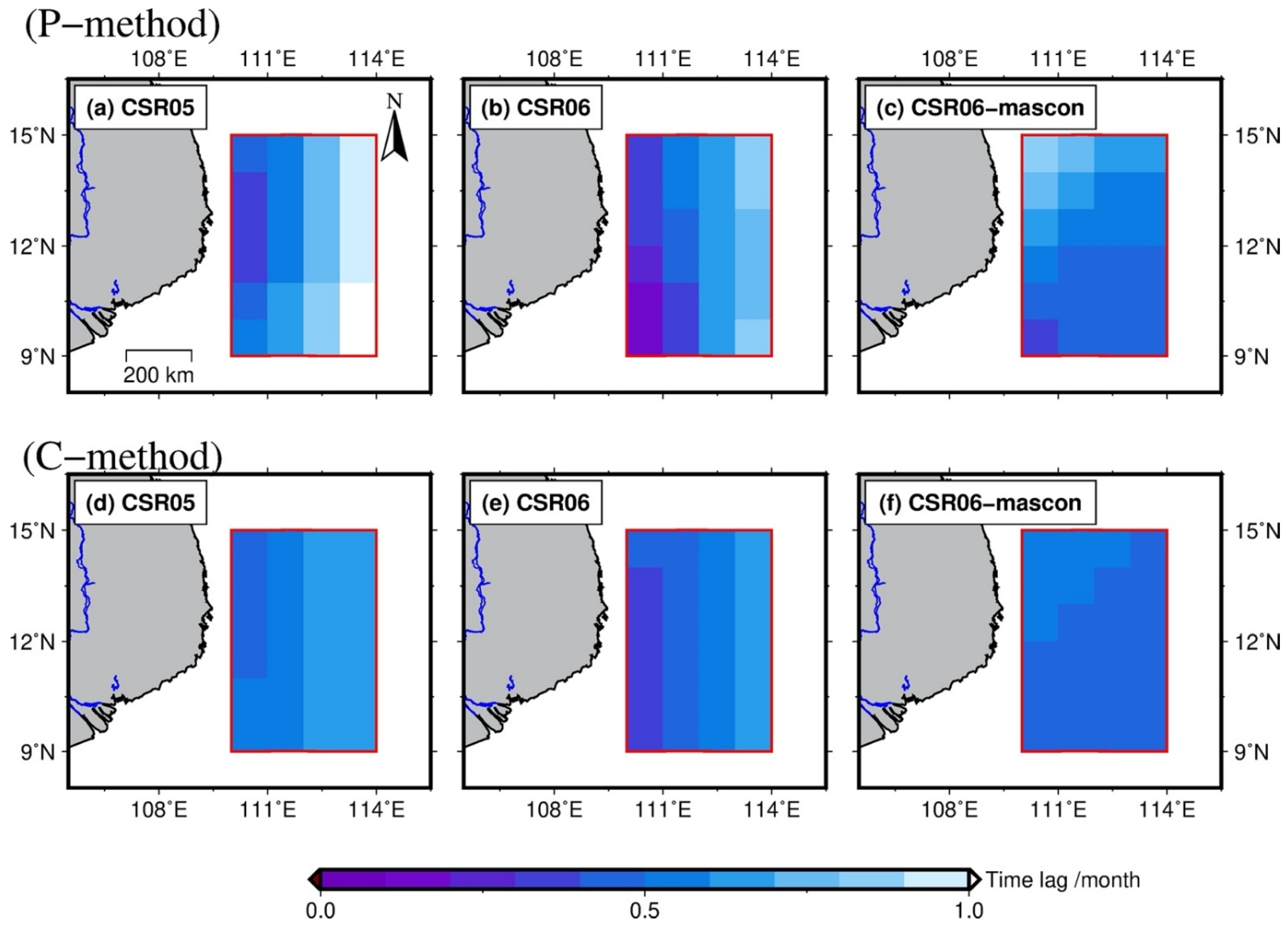
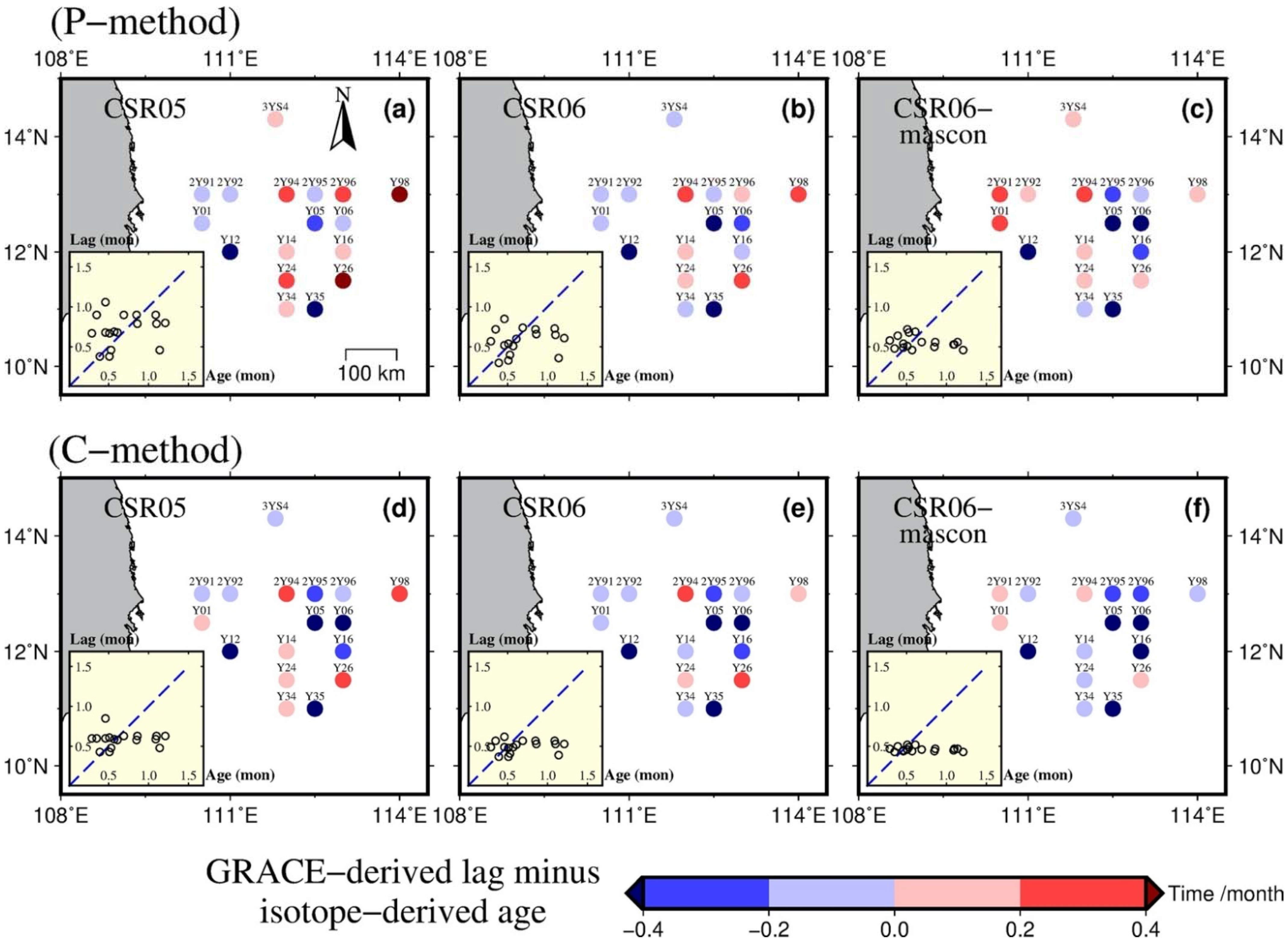
4.1. Regional Study Results by Phase Analysis (P-Method)

Employing the three-year rolling window, the three-year trend, annual amplitude and annual phase variation in runoff and EWHs are calculated for each three-year period during 2005–2012 (Figure 5). The time lag is derived by the annual phase difference between EWHs and in situ runoff. It should be noted that the values of CSR06-mascon annual amplitude are multiplied by two for a better visual expression of the annual amplitude in Figure 5b.

Table 1. The cross-correlation (PCC) between runoff and EWHs and their standard deviation (STD) from 2005 to 2012 in terms of three-year trend, annual amplitude and annual phase, in addition to the mean and STD of the time lag calculated by the annual phase difference between runoff and EWHs.

	Three-Year Trend (mm/month)		Annual Amplitude (mm)		Annual Phase (day)		Lag (day)
	PCC	STD	PCC	STD	PCC	STD	Mean	STD
runoff	--	0.25	--	1.23	--	1.33	--	--
CSR05	0.83	0.73	0.78	3.43	0.70	3.89	20	3.1
CSR06	0.92	0.79	0.64	2.83	0.48	5.21	17	4.8
CSR06-mascon	0.71	0.34	0.66	1.36	0.35	6.23	15	5.9

displays the PCC between runoff and EWH time series in terms of three-year trend, annual amplitude and annual phase variation, along with the calculated mean lag and corresponding standard deviation (STD).

During 2005–2008, the runoff and the CSR05 and CSR06 EWH trends increase slowly. However, no apparent change manifests for the CSR06-mascon EWH (Figure 5a). The three-year trend in EWHs and runoff rapidly decline when the rolling window starts to cover the time series of 2008 and 2009, reaching a minimum of ~–0.5 to –0.8 mm/month in 2009. This abrupt downward trend is speculated to be attributable to the moderate El Niño event during 2009–2010, which reduced seasonal rainfall, storage and runoff in the Mekong basin, as concluded from [37,53], thus weakening the Mekong river plume and its transport on the ocean surface. After this anomaly, the three-year trend in runoff and EWHs gradually increases and reaches the highest values, 0.5 mm/month and 1 mm/month, respectively. Among the three decomposed components of the EWH compared to those of the runoff, the highest PCC of 0.92 is attained for the CSR06 EWH in terms of three-year trend.

Within the time span shown in Figure 5b, the annual amplitude of runoff ranges from 36.15 to 42.28 mm, with the mean annual amplitude of ~49.9 mm and ~61.0 mm for CSR05 and CSR06, respectively, which values are approximately four times larger than that of CSR06-mascon (i.e., ~12.7 mm). These numerical differences in GRACE are mostly due to the different versions of the non-tidal oceanic and atmospheric model (i.e., AOD1B), corrected for CSR05 and CSR06, and the design of the regularization matrices for continental and oceanic areas for CSR06-mascon. The peaks and troughs of three EWHs are about 1~2 months later than the runoff time series. The PCCs between EWH and runoff in terms of annual amplitude are all higher than 0.60 (Table 1), and CSR05 EWH attains the highest PCC of 0.78.

On the contrary, the annual phase variations for the three EWHs are shown to be inconsistent with that of runoff, particularly in the ENSO event in 2010. During the El Niño event, the annual phase variation of the runoff was relatively small (Figure 5c), indicating the time lag determination by the annual phase difference would depend more on the EWH time series themselves, rather than on the in situ runoff. In general, the PCCs between all the three EWHs and the in situ runoff in terms of the annual phase were relatively lower than that of the three-year trend variation and annual amplitude (Table 1), showing the instability of the annual phase variation in freshwater mass as derived from GRACE in the open ocean. This inconsistency potentially reflects the time-varying influence of the ocean on Mekong freshwater transport. The mean and STD of the regional time lag are calculated in the last column of Table 1. Overall, the time lag estimated from CSR05 had the longest mean value (20 days) and the lowest STD (3.1 days).

4.2. Regional Study Results by Cross-Correlation Analysis (C-Method)

Using the C-method, the freshwater transport from estuary to our study region in the ocean has been determined by a proper δτ while maximizing the PCC(δτ) value. Again, employing the three-year rolling window, the original PCC with no lag (hereafter called oPCC), and the improved PCC (hereinafter called iPCC) with the proper time lag, δτ, are shown in the three EWH time series for each three-year period (Figure 6). Their corresponding mean values and STD are listed in

Table 2. The mean values and STDs of the original PCC (oPCC), the improved PCC (iPCC), and the lag between runoff and the three EWHs.

	oPCC		iPCC		Lag (in days)
	Mean	STD	Mean	STD	Mean	STD
CSR05	0.89	0.01	0.95	0.02	16	1.6
CSR06	0.91	0.03	0.96	0.01	15	2.1
CSR06-mascon	0.83	0.03	0.88	0.03	14	2.2

.

The oPCC values for three EWHs are all above 0.75 during the time span in our study, indicating their high relationship despite the time lag existing between EWHs and runoff. The mean improvement from oPCC to iPCC is ~0.05 in terms of three EWHs (Table 2), among which CSR06 yields the best correlation with runoff, with its iPCC reaching 0.96. The mean values of time lag are slightly smaller than that from the P-method, along with a smaller STD (i.e., ~2 days). Besides this, the time lag differences among the three EWHs are not apparent, with the highest time lag of 16 days for CSR05 and the lowest one of 14 days for CSR06-mascon. During the entire period, the mean and STD of the lag (Table 2) are all lower than those retrieved by the P-method (Table 1), which implies that the estimation by C-method was temporally smoother.

5. Discussion

Former isotope-derived ages in the western SCS measured between August and September 2007 [9] were employed to evaluate our time lag results for the two presented methods in the same region.

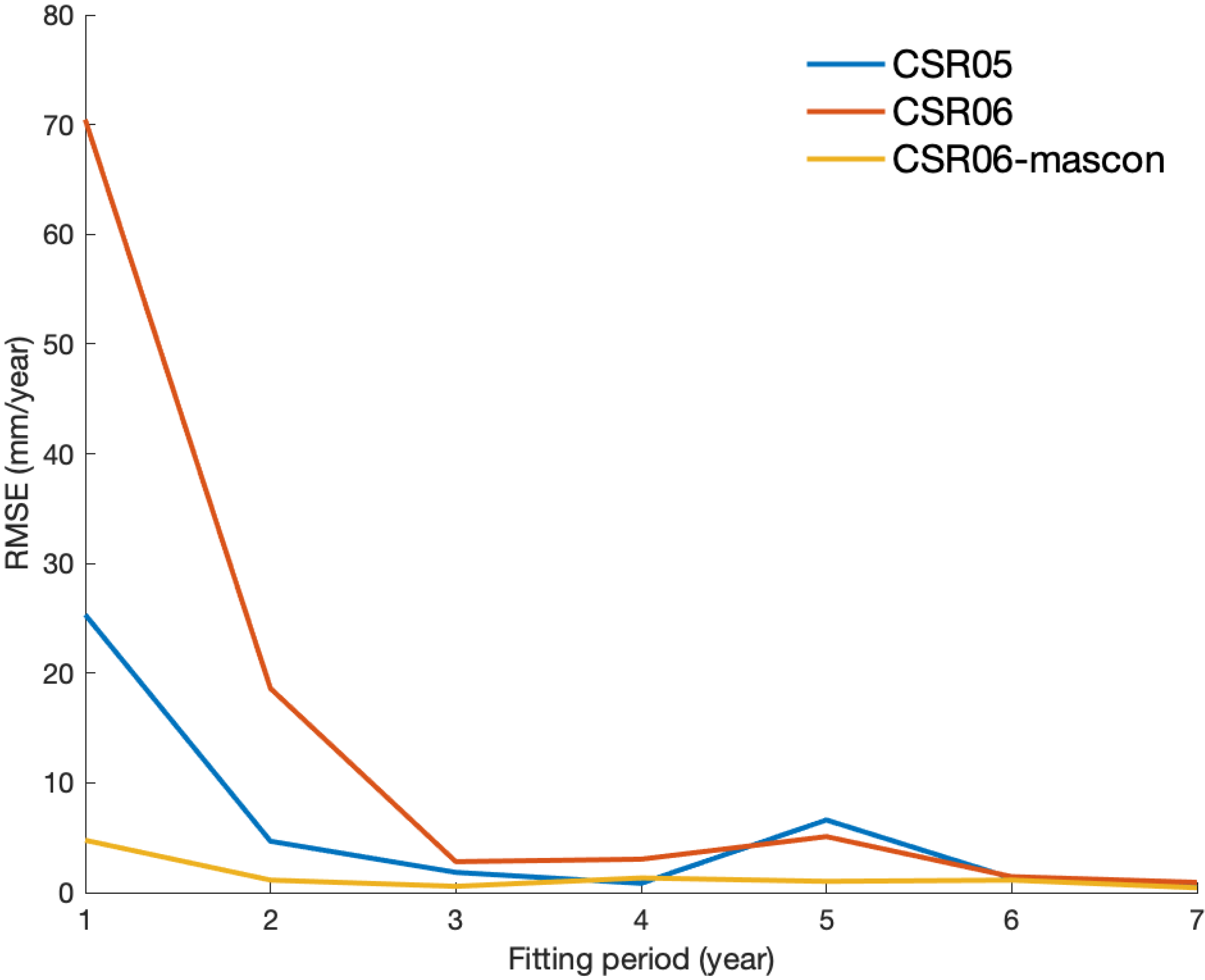
5.1. Gridded GRACE-Derived Time Lag Estimation by Two Methods

For evaluation, the time lags were determined using the P-method and the C-method in a three-year rolling window, with the median time epoch at 1 September 2007. Figure 7 presents the time lag results (in month) of each individual grid in the western SCS for the three EWHs derived by the P-method (Figure 7a–c) and the C-method (Figure 7d–f).

Among the six results, the gridded time lag from CSR06 using the P-method (Figure 7b) shows a clear eastward freshwater flowing path from the Mekong estuary along the Vietnam coastline to the ocean. The propagation was the integrated results of the seasonal offshore upper current [54,55], the monsoon [56], and ENSO events [57]. For the GRACE products, the gridded time lag results from CSR05 and CSR06 (Figure 7a,b,d,e) display several longitudinal panels parallel with the coastline, which were not evident from CSR06-mascon (Figure 7c,f). The existence of filtering for the Level-2 GRACE data might contribute to these differences. In terms of methodology, the spatial distribution of time lag using the C-method was smoother than that using the P-method, in addition to there being a narrower range of determined time lag. This indicates that the spatial distribution of the time lag retrieved from the EWHs and runoff time series depends not only on the GRACE data, but also on the methodologies themselves.

5.2. Comparison between GRACE-Derived Time Lag and Isotope-Derived Age

Figure 8 illustrates the difference between the isotope-derived age in September 2007 and the GRACE-derived time lag in the corresponding time span by the two presented methods. The time lag at the boundary of the GRACE grids is interpolated. Based on the scatter plots of time lag versus age, the time lag determined using the C-method fits the isotope-derived age better than that derived using the P-method, partially because the former method yields a narrower range of time lag. This result is particularly evident for the results from CSR06-mascon (Figure 8f), in which the lag clusters were approximately 0.5 months. However, in this case, the higher the age, the larger the discrepancy between the GRACE-derived time lag and the CSR06-mascon.

The differences between the GRACE-derived time lag and the isotope-derived age are displayed in colored dots at 17 selected stations (Figure 8). When the residual is larger than 0.2 months (i.e., 6 days) or smaller than –0.2 months, we consider the error was positively or negatively large, respectively. Based on this criterion, samplings with negatively large errors were observed mostly at locations away from the estuary (e.g., Y05, Y06, Y35), and so too were those with rather positively large errors (e.g., 2Y94, Y26, Y98). The high uncertainty of the end-member model used for calculating age by radium isotope partially contributes to these extremes. Besides this, a uniform time lag estimation by long-term time series analysis (i.e., three-year rolling window) is unable to detect short-term anomalies in the ocean. One example is the sampling station Y12, which displays an extremely old age because an eddy occurred nearby when the radium isotope was measured [9].

The mean and STD of age and time lag corresponding to all isotope samplings are listed in

Table 3. The mean and standard deviation of the isotope-derived age, the GRACE-derived lag, and their difference using the P-method and the C-method.

Estimation		Values		Lag Minus Age
		Mean	STD	Mean	STD
Isotope-derived age		0.68	0.29	--	--
GRACE-derived lag (P-method)	CSR05	0.71	0.19	0.03	0.32
	CSR06	0.58	0.15	–0.11	0.31
	CSR06-mascon	0.56	0.09	–0.13	0.33
GRACE-derived lag (C-method)	CSR05	0.59	0.09	–0.10	0.30
	CSR06	0.50	0.07	–0.18	0.29
	CSR06-mascon	0.46	0.02	–0.22	0.30

, in terms of GRACE data products and methods. Among the three GRACE data products, the mean of time lag derived from CSR05 approximates the mean of the isotope-derived age the most, with the differences of 0.03 months (i.e., 1 day) and –0.10 months (i.e., ~3 days) for the P-method and C-method, respectively. In terms of the methodology, the mean of time lag given by the P-method was slightly larger than that given by the C-method, which is consistent with our regional study results in Section 4.1. Additionally, the STD of the time lag minus age is ~0.3 months (i.e., 9 days), indicating that the quantitative comparison between time lag and age is greatly influenced by extreme values, partly because of the high uncertainty in the end-member model. Despite all these differences, the GRACE-derived time lag still fits properly with most isotope-derived ages, where the absolute errors are less than 0.2 months (i.e., 6 days). The paired t-test (

Table A3. The paired t-test results for GRACE-derived time lag and isotope-derived age based on the 17 selected isotope samples.

	P-Method			C-Method
	CSR05	CSR06	CSR06-Mascon	CSR05	CSR06	CSR06-Mascon
p	0.72	0.19	0.14	0.21	0.02	0.01

) does not reject the null hypothesis of their difference equaling zero at the 1% significance level (except results given by the C-method for CSR06-mascon).

According to measurements from Argo profiling floats during 2007, the mean surface velocity of the along-shore current was about 49 cm/s [58]. This means estuarine freshwater following this path would take about half a month to reach the center of our study area (i.e., ~700 km away from the estuary). This estimation was largely shown to be in agreement with our results and isotope-derived ages.

Overall, the GRACE-derived time lags are slightly smaller than the isotopic tracer ages. This could be partially caused by the deficiencies of our methods. For instance, the P-method depends on the length of data time span used for phase determination, whereas the C-method requires interpolation to the daily interval for the time shift in the cross-correlation analysis. The ages inferred from the isotope tracer analysis also suffer from the in situ measurement uncertainties, which are related to nearby ocean eddies and the highly sensitive end-member value determination process in the mixing model derived from [6]. Nonetheless, the results of both the methods presented in this study are more stable than those from the isotopic tracer analysis.

6. Conclusions

In this paper, the in situ runoff and GRACE product-derived freshwater mass in the ocean (EWHs) were used to determine the freshwater transport, in terms of time lag, from the Mekong river estuary to the western SCS via two independent methods: phase analysis (i.e., P-method) and cross-correlation analysis (i.e., C-method). A rolling data window was further applied to determine the time lag variation every three years during the period 2005–2012.

Among the three components (i.e., three-year trend, annual amplitude and phase) modeled in the P-method, EWHs correlated with runoff well in terms of trend and annual amplitude, with the minimum Pearson correlation coefficient (PCC) averaged for all three-year windows reaching 0.71 and 0.64, respectively. Inconsistency in the annual phase between runoff and EWHs potentially reflects the ocean’s influence on freshwater transport. Besides this, the differences resulting from three GRACE data products are apparent when climate extremes are encountered, for instance, a moderately strong El Niño event during the period 2009–2010. For the P-method, the average determined time lag of our study region was about 20, 17 and 15 days for CSR05, CSR06 and CSR06-mascon, respectively. In terms of the C-method, the mean PCC improvement was ~0.05 for three EWHs, and the determined time lag and its STD were relatively smaller compared with that derived from the P-method. The EWH value that correlated the best with runoff was given by CSR06, in which the mean PCC was improved from 0.91 to 0.96. Compared to the P-method, the fluctuation in time lag retrieved from the C-method was slightly lower in terms of both mean values and STD, thus weakening the difference caused by GRACE products.

To evaluate these two methods, the age results derived from radium isotope samplings in the western SCS by Chen et al. [9] in September 2007 were compared with our gridded time lag estimates whose median epoch in the rolling window was in the same month. Among the two methods, the time lag derived from the P-method showed a more distinguishable spatiotemporal pattern of freshwater propagation from the Mekong estuary toward the east, in particular CSR06. For the quantitative comparison against the GRACE-derived time lag, the isotope-derived age ranges were wider, showing a relatively high STD. This is partly due to high-frequency events (e.g., eddies) influencing isotope measurements, which cannot be recorded by GRACE. However, the isotope-derived age and GRACE-derived time lag still present a considerable agreement with each other, with over half the samplings showing small differences (i.e., ~6 days), regardless of the method. Overall, time lag determination by GRACE demonstrates a good potential for monitoring estuarine freshwater transport in the ocean. However, more experiments in different estuaries are required to further validate the universal feasibility of our presented analysis.

References

1. Johnston, R.M.; Kummu, M. Water Resource Models in the Mekong Basin: A Review. Water Resour. Manag. 2012, 26, 429–455. [Google Scholar] [CrossRef]
2. Hornerdevine, A.R.; Hetland, R.D.; Macdonald, D.G. Mixing and Transport in Coastal River Plumes. Annu. Rev. Fluid Mech. 2015, 47, 569–594. [Google Scholar] [CrossRef]
3. Chen, S. Enhancement of Alongshore Freshwater Transport in Surface-Advected River Plumes by Tides. J. Phys. Oceanogr. 2014, 44, 2951–2971. [Google Scholar] [CrossRef]
4. Hordoir, R.; Nguyen, K.D.; Polcher, J. Simulating tropical river plumes, a set of parametrizations based on macroscale data: A test case in the Mekong Delta region. J. Geophys. Res. 2006, 111. [Google Scholar] [CrossRef] [Green Version]
5. Schiller, R.V.; Kourafalou, V.H. Modeling river plume dynamics with the HYbrid Coordinate Ocean Model. Ocean Model. 2010, 33, 101–117. [Google Scholar] [CrossRef]
6. Moore, W.S.; Sarmiento, J.L.; Key, R.M. Tracing the Amazon component of surface Atlantic water using 228Ra, salinity and silica. J. Geophys. Res. Ocean 1986, 91, 2574–2580. [Google Scholar] [CrossRef] [Green Version]
7. Moore, W.S.; Krest, J. Distribution of 223Ra and 224Ra in the plumes of the Mississippi and Atchafalaya Rivers and the Gulf of Mexico. Mar. Chem. 2004, 86, 105–119. [Google Scholar] [CrossRef]
8. Xu, B.; Dimova, N.T.; Zhao, L.; Jiang, X.; Yu, Z. Determination of water ages and flushing rates using short-lived radium isotopes in large estuarine system, the Yangtze River Estuary, China. Estuar. Coast. Shelf Sci. 2013, 121, 61–68. [Google Scholar] [CrossRef]
9. Chen, W.; Liu, Q.; Huh, C.-A.; Dai, M.; Miao, Y.-C. Signature of the Mekong River plume in the western South China Sea revealed by radium isotopes. J. Geophys. Res. 2010, 115. [Google Scholar] [CrossRef] [Green Version]
10. Mccaul, M.; Barland, J.; Cleary, J.; Cahalane, C.; Mccarthy, T.J.; Diamond, D. Combining Remote Temperature Sensing with in-Situ Sensing to Track Marine/Freshwater Mixing Dynamics. Sensors 2016, 16, 1402. [Google Scholar] [CrossRef] [Green Version]
11. Gordon, H.R.; Morel, A. Remote Assessment of Ocean Color for Interpretation of Satellite Visible Imagery: A Review; Springer: New York, NY, USA, 1983. [Google Scholar]
12. Mullerkarger, F.E.; Mcclain, C.R.; Richardson, P.L. The dispersal of the Amazon’s water. Nature 1988, 333, 56–59. [Google Scholar] [CrossRef]
13. Gao, S.; Wang, H.; Liu, G.; Li, H. Spatio-temporal variability of chlorophyll a and its responses to sea surface temperature, winds and height anomaly in the western South China Sea. Acta Oceanol. Sin. 2013, 32, 48–58. [Google Scholar] [CrossRef]
14. He, Q.; Zhan, H.; Xu, J.; Cai, S.; Zhan, W.; Zhou, L.; Zha, G. Eddy-Induced Chlorophyll Anomalies in the Western South China Sea. J. Geophys. Res. 2019, 124, 9487–9506. [Google Scholar] [CrossRef]
15. Loisel, H.; Mangin, A.; Vantrepotte, V.; Dessailly, D.; Dinh, D.N.; Garnesson, P.; Ouillon, S.; Lefebvre, J.P.; Meriaux, X.; Phan, T.M. Variability of suspended particulate matter concentration in coastal waters under the Mekong’s influence from ocean color (MERIS) remote sensing over the last decade. Remote Sens. Environ. 2014, 150, 218–230. [Google Scholar] [CrossRef]
16. Loisel, H.; Vantrepotte, V.; Ouillon, S.; Ngoc, D.D.; Herrmann, M.; Tran, V.; Meriaux, X.; Dessailly, D.; Jamet, C.; Duhaut, T.; et al. Assessment and analysis of the chlorophyll-a concentration variability over the Vietnamese coastal waters from the MERIS ocean color sensor (2002–2012). Remote Sens. Environ. 2017, 190, 217–232. [Google Scholar] [CrossRef]
17. Tapley, B.D.; Watkins, M.M.; Flechtner, F.; Reigber, C.; Bettadpur, S.; Rodell, M.; Sasgen, I.; Famiglietti, J.S.; Landerer, F.W.; Chambers, D.P. Contributions of GRACE to understanding climate change. Nat. Clim. Chang. 2019, 9, 358–369. [Google Scholar] [CrossRef]
18. Alsdorf, D.; Lettenmaier, D.P. Tracking Fresh Water from Space. Science 2003, 301, 1491–1494. [Google Scholar] [CrossRef] [Green Version]
19. Schmidt, R.; Schwintzer, P.; Flechtner, F.; Reigber, C.; Guntner, A.; Doll, P.; Ramillien, G.; Cazenave, A.; Petrovic, S.; Jochmann, H. GRACE observations of changes in continental water storage. Glob. Planet. Chang. 2006, 50, 112–126. [Google Scholar] [CrossRef]
20. Wouters, B.; Bonin, J.A.; Chambers, D.P.; Riva, R.E.M.; Sasgen, I.; Wahr, J. GRACE, time-varying gravity, Earth system dynamics and climate change. Rep. Prog. Phys. 2014, 77, 41. [Google Scholar] [CrossRef] [PubMed] [Green Version]
21. Ramillien, G.; Famiglietti, J.S.; Wahr, J. Detection of Continental Hydrology and Glaciology Signals from GRACE: A Review. Surv. Geophys. 2008, 29, 361–374. [Google Scholar] [CrossRef]
22. Volkov, D.L.; Landerer, F.W. Nonseasonal fluctuations of the Arctic Ocean mass observed by the GRACE satellites. J. Geophys. Res. 2013, 118, 6451–6460. [Google Scholar] [CrossRef]
23. Tregoning, P.; Lambeck, K.; Ramillien, G. GRACE estimates of sea surface height anomalies in the Gulf of Carpentaria, Australia. Earth Planet. Sci. Lett. 2008, 271, 241–244. [Google Scholar] [CrossRef]
24. Wouters, B.; Chambers, D. Analysis of seasonal ocean bottom pressure variability in the Gulf of Thailand from GRACE. Glob. Planet. Chang. 2010, 74, 76–81. [Google Scholar] [CrossRef]
25. Chen, Y.; Fok, H.S.; Ma, Z.; Tenzer, R. Improved Remotely Sensed Total Basin Discharge and its Seasonal Error Characterization in the Yangtze River Basin. Sensors 2019, 19, 3386. [Google Scholar] [CrossRef] [PubMed] [Green Version]
26. Liu, Y.-C.; Hwang, C.; Han, J.; Kao, R.; Wu, C.-R.; Shih, H.-C.; Tangdamrongsub, N. Sediment-Mass Accumulation Rate and Variability in the East China Sea Detected by GRACE. Remote Sens. 2016, 8, 777. [Google Scholar] [CrossRef] [Green Version]
27. Chen, J.L.; Wilson, C.R.; Li, J.; Zhang, Z. Reducing leakage error in GRACE-observed long-term ice mass change: A case study in West Antarctica. J. Geod. 2015, 89, 925–940. [Google Scholar] [CrossRef]
28. Dobslaw, H.; Dill, R.; Bagge, M.; Klemann, V.; Boergens, E.; Thomas, M.; Dahle, C.; Flechtner, F. Gravitationally Consistent Mean Barystatic Sea Level Rise from Leakage-Corrected Monthly GRACE Data. J. Geophys. Res. Solid Earth 2020, 125. [Google Scholar] [CrossRef]
29. Mu, D.; Xu, T.; Xu, G. Detecting coastal ocean mass variations with GRACE mascons. Geophys. J. Int. 2019, 217, 2071–2080. [Google Scholar] [CrossRef]
30. Kummu, M.; Varis, O. Sediment-related impacts due to upstream reservoir trapping, the Lower Mekong River. Geomorphology 2007, 85, 275–293. [Google Scholar] [CrossRef]
31. Cochrane, T.A.; Arias, M.E.; Piman, T. Historical impact of water infrastructure on water levels of the Mekong River and the Tonle Sap system. Hydrol. Earth Syst. Sci. 2014, 18, 4529–4541. [Google Scholar] [CrossRef] [Green Version]
32. Dang, V.H.; Tran, D.D.; Pham, T.B.T.; Khoi, D.N.; Tran, P.H.; Nguyen, N.T. Exploring Freshwater Regimes and Impact Factors in the Coastal Estuaries of the Vietnamese Mekong Delta. Water 2019, 11, 782. [Google Scholar] [CrossRef] [Green Version]
33. Xue, Z.; Liu, J.P.; Ge, Q. Changes in hydrology and sediment delivery of the Mekong River in the last 50 years: Connection to damming, monsoon, and ENSO. Earth Surf. Process. Landf. 2011, 36, 296–308. [Google Scholar] [CrossRef]
34. Zhu, Y.; Fang, G.; Wei, Z.; Wang, Y.; Teng, F.; Qu, T. Seasonal variability of the meridional overturning circulation in the South China Sea and its connection with inter-ocean transport based on SODA2.2.4. J. Geophys. Res. Oceans 2016, 121, 3090–3105. [Google Scholar] [CrossRef] [Green Version]
35. Quan, Q.; Xue, H.; Qin, H.; Zeng, X.; Peng, S. Features and variability of the South China Sea western boundary current from 1992 to 2011. Ocean Dyn. 2016, 66, 795–810. [Google Scholar] [CrossRef]
36. Wu, W.; Wang, L.; Liao, Y.; Huang, B. Microbial eukaryotic diversity and distribution in a river plume and cyclonic eddy-influenced ecosystem in the South China Sea. MicrobiologyOpen 2015, 4, 826–840. [Google Scholar] [CrossRef]
37. Rasanen, T.A.; Kummu, M. Spatiotemporal influences of ENSO on precipitation and flood pulse in the Mekong River Basin. J. Hydrol. 2013, 476, 154–168. [Google Scholar] [CrossRef]
38. Da, N.D.; Herrmann, M.; Morrow, R.; Nino, F.; Huan, N.M.; Trinh, N.Q. Contributions of wind, ocean intrinsic variability and ENSO to the interannual variability of the South Vietnam Upwelling: A modeling study. J. Geophys. Res. 2019, 124, 6545–6574. [Google Scholar] [CrossRef]
39. Save, H.; Bettadpur, S.; Tapley, B.D. High-resolution CSR GRACE RL05 mascons. J. Geophys. Res. Solid Earth 2016, 121, 7547–7569. [Google Scholar] [CrossRef]
40. Save, H. CSR GRACE RL06 Mascon Solutions, Texas Data Repository, V1. 2019. Available online: https://doi.org/10.18738/T8/UN91VR (accessed on 12 March 2021).
41. Bettadpur, S. Level-2 Gravity Field Product User Handbook; Center for Space Research the University of Texas at Austin: Austin, TX, USA, 2018. [Google Scholar]
42. Chambers, D.P.; Bonin, J.A. Evaluation of Release-05 GRACE time-variable gravity coefficients over the ocean. Ocean Sci. 2012, 8, 859–868. [Google Scholar] [CrossRef] [Green Version]
43. Dobslaw, H.; Flechtner, F.; Bergmann-Wolf, I.; Dahle, C.; Dill, R.; Esselborn, S.; Sasgen, I.; Thomas, M. Simulating high-frequency atmosphere-ocean mass variability for dealiasing of satellite gravity observations: AOD1B RL05. J. Geophys. Res. Oceans 2013, 118, 3704–3711. [Google Scholar] [CrossRef] [Green Version]
44. Cheng, M.; Tapley, B.D. Variations in the Earth’s oblateness during the past 28 years. J. Geophys. Res. Solid Earth 2004, 109. [Google Scholar] [CrossRef]
45. Swenson, S.; Chambers, D.; Wahr, J. Estimating geocenter variations from a combination of GRACE and ocean model output. J. Geophys. Res. Solid Earth 2008, 113, 08410. [Google Scholar] [CrossRef] [Green Version]
46. Ries, J.B.; Bettadpur, S.; Eanes, R.; Kang, Z.; Ko, U.; McCullough, C.; Nagel, P.; Pie, N.; Poole, S.; Richter, T.; et al. The Combined Gravity Model GGM05C; GFZ Data Services: Potsdam, Germany, 2016. [Google Scholar]
47. Swenson, S.; Wahr, J. Post-processing removal of correlated errors in GRACE data. Geophys. Res. Lett. 2006, 33. [Google Scholar] [CrossRef]
48. Broerse, T.; Riva, R.; Simons, W.; Govers, R.; Vermeersen, B. Postseismic GRACE and GPS observations indicate a rheology contrast above and below the Sumatra slab. J. Geophys. Res. Solid Earth 2015, 120, 5343–5361. [Google Scholar] [CrossRef] [Green Version]
49. Fok, H.S.; Zhou, L.; Liu, Y.; Ma, Z.; Chen, Y. Upstream GPS Vertical Displacement and its Standardization for Mekong River Basin Surface Runoff Reconstruction and Estimation. Remote Sens. 2020, 12, 18. [Google Scholar] [CrossRef] [Green Version]
50. Moore, W.S.; Todd, J.F. Radium isotopes in the Orinoco estuary and eastern Caribbean Sea. J. Geophys. Res. Oceans 1993, 98, 2233–2244. [Google Scholar] [CrossRef]
51. Bruner de Miranda, L.; Pinheiro Andutta, F.; Kjerfve, B.; de Castro Filho, B.M. Fundamentals of Estuarine Physical Oceanography; Springer: Singapore, 2017. [Google Scholar]
52. Li, Z.; Zhang, C.; Ke, B.; Qiao, L.; Li, W.; Liu, Y. Inversion for sediment variation in the East China Sea using GRACE data. Chin. J. Geophys. Chin. Ed. 2019, 62, 2429–2440. [Google Scholar]
53. Amarasekera, K.N.; Lee, R.; Williams, E.; Eltahir, E.A.B. ENSO and the natural variability in the flow of tropical rivers. J. Hydrol. 1997, 200, 24–39. [Google Scholar] [CrossRef]
54. Fang, W.; Fang, G.; Shi, P.; Huang, Q.; Xie, Q. Seasonal structures of upper layer circulation in the southern South China Sea from in situ observations. J. Geophys. Res. 2002, 107, 3202. [Google Scholar] [CrossRef]
55. Zu, T.; Wang, D.; Wang, Q.; Li, M.; Wei, J.; Geng, B.; He, Y.; Chen, J. A revisit of the interannual variation of the South China Sea upper layer circulation in summer: Correlation between the eastward jet and northward branch. Clim. Dyn. 2020, 54, 457–471. [Google Scholar] [CrossRef]
56. Chen, C.; Wang, G. Interannual variability of the eastward current in the western South China Sea associated with the summer Asian monsoon. J. Geophys. Res. Oceans 2014, 119, 5745–5754. [Google Scholar] [CrossRef]
57. Wang, C.; Wang, W.; Wang, D.; Wang, Q. Interannual variability of the South China Sea associated with El Niño. J. Geophys. Res. Oceans 2006, 111. [Google Scholar] [CrossRef]
58. Zhou, H.; Yuan, D.; Li, R.; He, L. The western South China Sea currents from measurements by Argo profiling floats during October to December 2007. Chin. J. Oceanol. Limnol. 2010, 28, 398–406. [Google Scholar] [CrossRef]
Figure 1. Lower Mekong basin and southern SCS. Dashed boundary (on the right) is our regional study area with selected (red dots) and unselected (grey dots) isotope samplings, along with their sampling codes (above the dots) and age (in month) (below the dots) (adapted with permission from ref. [9], Copyright 2010 American Geophysical Union).
Remotesensing 13 01193 g001
Figure 2. A flow chart of GRACE further processes from GSM to EWH on CSR05, CSR06 and CSR06-mascon. GSM, GRACE geopotential coefficients after priori models corrections; GGM05C, a combination global gravity model; EWH, equivalent water height.
Remotesensing 13 01193 g002
Figure 3. The average gridded EWH time series for GRACE CSR05, CSR06 and CSR06-mascon data products over 9–15°N, 110–114°E in the western SCS during 2005–2012.
Remotesensing 13 01193 g003
Figure 4. Monthly Mekong basin runoff measured at the Chau Doc and Tan Chau stations during 2005–2012.
Remotesensing 13 01193 g004
Figure 5. Time series of three versions of GRACE EWHs against runoff employing three-year rolling windows during 2005–2012 in terms of (a) three-year trend, (b) annual amplitude and (c) annual phase. Note that the annual amplitude of CSR06-mascon was doubled in (b). The x-axis labels each complete three-year period. For example, “2005–2007” represents the time period between January 2005 and December 2007.
Remotesensing 13 01193 g005
Figure 6. The original Pearson correlation coefficient (PCC) (solid line) and improved PCC (dotted line) between the runoff and (a) CSR05, (b) CSR06, and (c) CSR06-mascon EWHs via the three-year rolling window using the C-method. The gray bar represents the corresponding time lag. The x-axis labels complete three-year periods. For example, “2005–2007” represents the time period between January 2005 and December 2007.
Remotesensing 13 01193 g006
Figure 7. Spatial distribution of time lag for CSR05, CSR06 and CSR06-mascon using the P-method (ac) and C-method (df), respectively, between March 2006 and February 2009, such that the median time epoch is 1 September 2007.
Remotesensing 13 01193 g007
Figure 8. Difference between GRACE-derived time lag and isotope-derived age for 17 selected isotope samplings. Note that the GRACE-derived time lag was calculated from CSR05, CSR06 and CSR06-mascon using the P-method (ac) and the C-method (df), respectively. The subgraphs (bottom left) plot the scatterings of the corresponding time lag and age from the different versions of GRACE data, derived using the P-method and the C-method.
Remotesensing 13 01193 g008