Abstract
As a vital role in the processes of the energy balance and hydrological cycles, actual evapotranspiration (ET) is relevant to many agricultural, ecological and water resource management studies. The available global or regional ET products provide ET estimations with various temporal ranges, spatial resolutions and calculation methods (algorithms, inputs and parameterization, etc.), leading to varying degrees of introduced uncertainty. Northern China is the main agriculturally productive region supporting the whole country; thus, understanding the spatial and temporal changes in ET is essential to ensure water resource and food security. We developed a synthesis ET dataset for Northern China at a 1000 m spatial resolution, with a monthly temporal resolution covering a period ranging from 1982 to 2017, using an in-depth assessment of several ET products. Specifically, assessments were performed using in situ measured ET from eddy covariance (EC) observation towers at the site-pixel scale over interannual months under the conditions of different land cover types, climatic zones and elevation levels to select the most optimally performing ET products to be used in the synthesized ET dataset. Eight indicators under 21 conditions were involved in the assessment sheet, while the statistics of the different ET product occurrences and corresponding ratios were analyzed to select the best-performing ET products to build the synthesis ET dataset using the weighted mean method. The weights were determined by the Taylor skill score (TSS), calculated with ET products and EC ET observation data. Based on the assessment results, the Penman–Monteith–Leuning (PML_v2), ETWatch and Operational Simplified Surface Energy Balance (SSEBop) datasets were selected for implementation in the synthesis ET dataset from 2003 to 2017, while Global Land Evaporation Amsterdam Model (GLEAM) v3.3a, complementary relationship (CR) ET, and Numerical Terradynamic Simulation Group (NTSG) datasets were chosen for the synthesis ET dataset from 1982 to 2002. The weighted mean synthesized results from 2003 to 2017 performed well when compared to the in situ measured EC ET values produced under all of the above conditions, while the synthesized results from 1982 to 2002 performed well through the water balance method in Heihe River Basin. These results can provide more stable ET estimations for Northern China, which can contribute to relevant agricultural, ecological and hydrological studies.
1. Introduction
Evapotranspiration (ET) is a process in which liquid or solid water is converted into water vapor after precipitation reaches the ground during the hydrological cycle and returns to the atmosphere [1,2,3]; it mainly involves surface water, soil water evaporation and vegetation canopy transpiration [4,5]. From a global perspective, two-thirds of precipitation is returned to the atmosphere by evapotranspiration [6]. Therefore, ET is a critical component of terrestrial ecosystems and profoundly impacts the water balance and energy cycle of the terrestrial surface [7,8]. Accurate ET estimates are vital to study hydrological processes from basin to regional levels [9,10,11,12,13], global climate change [14,15,16,17], drought and flood monitoring [18,19,20], water resource and optimal allocation management [21,22,23,24], agricultural water management and irrigation scheduling [25,26,27,28], environmental protection and ecological restoration [29,30]. Northern China has a complicated terrain and a large east–west span and is the country’s main wheat and corn production area [31]. Food security in this region is primarily dependent on water resource security, because most of the cultivated land is irrigated [32]. From a regional perspective, water is mainly sourced from precipitation, and evapotranspiration and river flow are the leading causes of water loss [33]. Hence, understanding temporal and spatial changes in ET is crucial to water resource and food security in Northern China. In situ ground measurement methods of ET using observational instruments, such as Bowen ratio (BR) systems [34], eddy covariance (EC) systems [35] and lysimeters [36], are widely applied across relevant research areas. Although the true value of ET can be obtained at the observed time and representative spatial extent, the spatial representativeness is limited to a certain point or within a small area, while large-scale observations are expensive [37]. Simulation methods based on remotely-sensed data are more effective in obtaining the spatial distribution of ET and guarantee temporal continuity [38].
Recently, various remote sensing-based global ET datasets have been generated using different mechanisms. Some are remote sensing diagnostic products based on the surface energy balance (SEB), in which the thermal infrared band plays a significant role [28,39] and can be denoted as the Penman–Monteith–Leuning evapotranspiration V2 (PML_V2) [40], Surface Energy Balance System (SEBS) [41], Operational Simplified Surface Energy Balance (SSEBop) [42], the Moderate Resolution Imaging Spectroradiometer (MODIS) Global Evapotranspiration Project (MOD16) [43], etc. ET datasets generated with the land surface model (LSM) that describe land surface processes that have a great impact on the Earth system and govern the exchanges of heat, moisture and momentum between the surface and atmosphere [44] are represented by the Global Land Evaporation Amsterdam Model (GLEAM) v3.3a [45], Global Land Data Assimilation System (GLDAS) [46], and Famine Early Warning Systems Network (FEWS NET) Land Data Assimilation System (FLDAS) [47]. Additionally, there are also ET datasets that have been developed from hydrological models, such as TerraClimate, in which the actual ET is derived from a one-dimensional soil water balance model [48]. For regional ET datasets covering Northern China, the representatives include the ETWatch product [49], an operational ET product based on the surface energy balance and Penman–Monteith (PM) equation, and CR ET product [50], a complementary relationship (CR)-based diagnostic ET product for the Chinese terrestrial surface.
The available ET products differ in their model inputs, parameterizations and algorithms, leading to varying degrees of uncertainties [51,52]. Thus, it is challenging to select a proper ET dataset that accurately represents the hydroclimatic features of a region [49]; therefore, the evaluation of ET results is essential to ensure reliability [53]. Among the evaluation methods, EC in situ field measurements and hydrological records are most widely applied as reference data for validating various ET estimates at the pixel and basin-wide levels, respectively, in various ET-related studies [54,55,56,57,58]. Focusing on Northern China, the ETWatch in the Hai River basin and CR ET products have been validated by comparing field flux measurements and hydrological records with model estimations [50,59,60].
Given the uncertainties in different ET products, several data fusion methods, such as simple model averaging (SMA) [61,62], Bayesian model averaging (BMA) [63,64] and the simple Taylor skill (STS) method [65,66], were applied to blend the different ET products to build an ensemble ET dataset to reduce uncertainties, and better performances were found in the ensemble dataset. Ershadi et al. [62] determined that the ensemble dataset had the lower uncertainty level when compared with other member ET products; according to their Nash–Sutcliffe efficiency (NSE) and root mean squared difference (RMSD) values. Yang et al. [63] applied the BMA method and merged eight satellite-based ET datasets and attributed the highest accuracy to an ensemble with four models (Reg2, PT-JPL, RRS-PM and MODIS ET). In the study by Niyogi et al. [67], different statistical metrics, including STS, have been applied to compare satellite-based and land surface-based ET datasets, from which the combination of MODIS ET and the GLEAM dataset could generate the most accurate ET estimates in the United States. Other studies (e.g., Yao et al. [65], Vinukollu et al. [61], Mueller et al. [68], Badgley et al. [69], and Jiang et al. [70]) have applied multidata set synthesis and generated regional and global ET datasets with different degrees of bias. From our perspective, this research aims to provide an assessment-based synthesis scheme with a Taylor skill score (TSS)-based weight and establish a synthesis ET dataset within Northern China. Validations at the site–pixel scale and intercomparison among different global and local ET products are carried out with in situ EC measurements over different land cover types, elevation scales and climatic zones to select the ET datasets with the best performance over these varied conditions for further synthesis, which can obtain a better understanding of the validity and characteristics of the different ET datasets in Northern China. Conversely, the above selected ET products represent the optimally performing products within Northern China and can be synthesized using TSS-based weight for monthly ensemble ET datasets.
2. Study Area and Data
2.1. Study Area
Eighteen Chinese provinces were taken into consideration as the defined study area and comprised northern, northeastern, and some parts in the northwestern, eastern and central regions of China. The provinces of Heilongjiang, Liaoning, Jilin, Xinjiang, Inner Mongolia, Hebei, Shanxi, Shandong, Ningxia, Beijing and Tianjin are fully encompassed, while the Qinghai, Gansu, Shaanxi, Henan, Hubei, Anhui and Jiangsu Provinces are partially covered. The spatial extent covers a latitude ranging from 28.02°N to 54.21°N and a longitude ranging from 71.37°E to 136.72°E. The land area covers 5.53 million km2, accounting for 57.6% of the country’s total area. Most of the study area is located in the temperate zone, and the climatic zone is humid, semihumid, semiarid and arid from east to west. Generally, the land cover types in Northern China are unique and complex, with mountains, plateaus, basins, hills and plains and many different types of vegetation (Figure 1). In addition, Northern China is agriculturally vital and is where a majority of the wheat and corn resources are produced [32].
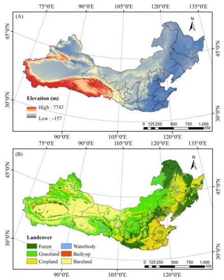
Figure 1.
(A) Location of Northern China with elevation. (B) Land cover map for Northern China.
2.2. Data
2.2.1. Evapotranspiration
Eleven global and two local actual ET datasets were collected for this research. The ET estimations from FLDAS, GLDAS_V20 and GLDAS_V21 are all LSM-based, and the Penman–Monteith (PM) or Priestley–Taylor (PT) equations are involved in the processing of the other 10 ET products. Among these 10 ET products, MOD16A2 (both Collection 6 (C6) and Collection 5 (C5)), PML_V2 and NTSG are mainly based on the specific canopy conductance model, while SEBS, SSEBop and ETWatch are mainly based on the surface energy balance. In particular, GLEAM (both 3.3a and 3.3b) utilizes the soil stress factor in the conversion from potential ET to actual ET, and CR_ET mainly utilizes the complementary relationship (CR) between actual and potential ET. ET products collected had different spatiotemporal resolutions and temporal range, and the specifications of the abovementioned ET products are summarized in Table 1.

Table 1.
Summary of the abovementioned evapotranspiration (ET) products.
2.2.2. ET Tower Observation Data
ET tower observations from 18 EC flux sites were processed monthly as reference data for validating and assessing the ET products described above. Among them, five sites are from AsiaFlux (https://www.asiaflux.net/ access: 10 March 2021), five sites are from ChinaFlux (https://www.chinaflux.org/ access: 10 March 2021), four sites are from FluxNET (https://fluxnet.fluxdata.org/ access: 10 March 2021) and four sites are from the Aerospace Information Research Institute, Chinese Academy of Sciences (AIRCAS). The periods of flux EC data range from 1 year (12 months) to 8 years (96 months), while the temporal scale of the processed monthly ET values of all the sites ranges from 2002 to 2017. In total, there are 782 site months. The EC flux sites are distributed across different underlying surfaces, marked by various land cover types using the International Geosphere–Biosphere Programme (IGBP) classification system. The 18 EC flux sites mainly cover five vegetation types: deciduous needle leaf forest (DNF, one site), mixed forest (MF, two sites), cropland (CRO, six sites) and grassland (GRA, nine sites). The information for each flux site is summarized in the following Table 2.
Table 2.
Summary of the flux site data.
The collected EC flux data are averaged every half hour in a text format, and the gap-filling method is applied throughout the process [71]. Then, the gap-filled half-hourly averaged latent heat flux is aggregated to obtain the monthly ET. The conversion between latent heat flux and ET is calculated using Equation (1) [72]:
where LE (W·m−2s−1) is the latent heat flux, and λ is the latent heat of evaporation. Air temperature is the main factor influencing λ, but variability in air temperature only causes minor changes in λ [73]. In view of the limited influence of air temperature on the estimated ET values with LE [74,75], a constant value of 2.45 MJ·kg−1 is used in the Equation (1) [73].
2.2.3. Auxiliary Data
The main auxiliary data involved in this study are digital elevation model (DEM), aridity index (AI) and gridded precipitation datasets. DEM data are extracted from the 1 arc-second void-filled Shuttle Radar Topography Mission (SRTM) v3 product provided by NASA JPL, which covers the land surface area between 56°S and 60°N in altitude, accounting for approximately 80% of the total land area of Earth [76]. The AI dataset is defined as the mean annual precipitation divided by the mean annual evapotranspiration, the former of which is extracted from the WorldClim global climate dataset, and the latter is simulated by the Hargreaves equation [77], the spatial resolution of which is 30 arc-seconds (https://cgiarcsi.community/data/global-aridity-and-pet-database access: 10 March 2021). Precipitation data is extracted from the gridded precipitation dataset produced by the China Meteorological Data Service Center (CMDC) [78], which is generated by spatial interpolation method of the Thin Plate Spline (TPS) using the latest precipitation data of 2472 stations with the spatial resolution of 0.5°, spanning from 1961 to the latest. DEM and AI data were mainly for the stratifications of flux sites, while precipitation data were used for water balance assessment.
3. Method
3.1. Assessment Method
Due to the complexity of land–atmosphere interactions and their various simulation mechanisms, ET is extremely variable over time and space between the different product datasets, and their performances can be very diverse under different underlying surface conditions, so it is necessary to use ground observation data for comprehensive evaluation [62,76,79,80]. A set of indicators was applied in the comprehensive assessment of the different ET products. Mean error (ME), mean absolute error (MAE) and root mean square error (RMSE) are the most commonly used error measure indicators. ME and MAE, used as bias indicators, represent the average error and absolute error between the ET product values and the tower observed values, respectively, while RMSE represents the sample standard deviation of the difference between the ET product values and the observed values, reflecting the accuracy of ET products. The ME results can indicate whether overestimation or underestimation occurs, whereas the MAE results can avoid the mutual cancelation of errors, which can accurately reflect the actual forecast error. As mentioned in Rim’s article [81], RMSE is more sensitive to outliers than MAE, because a single error measured with RMSE increases quadratically, and MAE is a more direct measurement excluding exponential operations; however, RMSE is generally more adaptable to in-depth statistical analyses of error than MAE. Despite these differences, ME, MAE and RMSE all measure the average difference, and it is suitable to utilize each index. As a result of the variability of ET measurements, it is difficult to evaluate the accuracy of ET products using only direct error measures such as ME, MAE and RMSE, and, therefore, their relative values, including the relative mean error (RME), relative mean absolute error (RRMAE) and relative root mean square error (RRMSE), are simultaneously reported [80,82,83]. Moreover, the Pearson correlation coefficient (R) is used as a statistical indicator to measure the strength of the relationship between the different ET products and observed ET values [58], and Willmott’s index of agreement (d) is used to describe how well the model-calculated results simulate the observed data [84]. The indicators are calculated using Equations (2)–(9):
where n is the record number; is the i-th record; is the mean value of the observed ET dataset and is the mean ET of the different ET products.
The aridity index, elevation and ET values from the different product datasets are extracted as data records for the positions of each flux tower. To carry out a comprehensive assessment, the accuracy of the different ET products is evaluated using the eight indicators mentioned above from the perspectives of climatic zones, land cover types and elevation levels with the following stratifications (Table 3): The aridity index (AI) is classified into three classes, including dry subhumid, humid and semiarid groups, using the United Nations Environment Programme definitions [85] to describe the different climatic zones. The IGBP land cover type of every flux tower position is aggregated into three types: forest, grassland and cropland. The elevation is aggregated into three levels: low, medium and high. The performances of ET products determined using different indicators under different conditions will be displayed in the assessment sheet, which is described in Section 4.2 in detail.
Table 3.
Stratifications of different climatic zones, land cover types and elevation levels.
3.2. Synthesis and Validation Method
Through a series of comprehensive assessments, the highly ranked ET products can be selected according to the assessment results. To harmonize the spatial temporal resolution of selected ET datasets, the ET dataset that had finer temporal resolution than a month were all aggregated to monthly time step. Furthermore, ET datasets with spatial resolution finer than 1 km were resampled to 1 km with pixel average, while coarser ET datasets were resampled to 1 km with nearest neighborhood. For the synthesis of the selected datasets, the weighted mean strategy was applied. The weight of the different selected ET datasets is determined by the calculated Taylor skill scores (TSS) [86]. The weights of every individual ET product, which are proportional to the TSS values, are added to 1 [65]. The calculation of the TSS and weights for the different ET datasets and the TSS-based synthesis method are expressed as Equations (10)–(12):
where TSSi is the Taylor skill score for an ET product i; n is the number of ET products; Ri is the Pearson correlation coefficient between an ET product i and the in situ measured EC ET; Rmax represents the maximum correlation coefficient and is set to 1 in this research; δi is the ratio of the standard deviation of ET product i to the in situ measured EC ET; wi is the TSS-based weight for ET product I; ETi is the i-th ET product; and ETsyn is the synthesis result with the weighted mean of the ET products. The TSS values range from 0 to 1, where 0 and 1 indicate the least skillful and most skillful datasets, respectively.
As for validation of the synthesized results, EC ET was used with the assessment sheet proposed in Section 3.1, while the gridded precipitation was involved in the water balance assessment of the synthesized results (in Section 4.4).
The overall methodology of this study is concluded as the following flow chart (Figure 2).
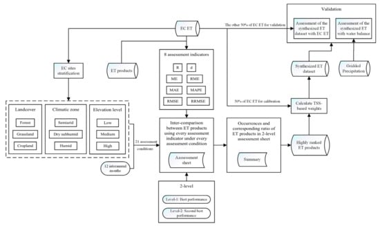
Figure 2.
Flow chart of methodology for this study.
4. Results
4.1. Assessment of ET Products from Different Perspectives
Figure 3 shows the multiyear monthly average of each ET product under different conditions as well as the observed flux EC ET. As seen from the EC ET, obvious seasonal changes were captured. For all sites’ averages (Figure 3A), the ET values from April to September are relatively high (higher than 40 mm), and the peak value is 91.36 mm in July. Regarding the different ET products, nearly all of them captured seasonal changes. FLDAS, GLDAS_v20, GLDAS_v21, MOD16A2_C6 and NTSG reported maximum values in August ranging from 66.10 mm (MOD16A2_C6) to 108.89 mm (FLDAS), while the other ET products had maximum values in July ranging from 63.95 mm (SEBS) to 105.68 mm (ETWatch). Winter wheat is widely cultivated throughout the plain area of Northern China and is harvested in June. Then, corn is sowed following winter wheat. Therefore, the ET in June in these areas is typically smaller than that in the adjacent two months, which was sufficiently captured by Figure 3D,H. From Figure 3B–J, it is apparent that MOD16A2_C6 generally reported the smallest values from June to July, excluding sites under the conditions of grassland, dry subhumid regions and elevations greater than 1500 m. In contrast, the SSEBop dataset significantly overestimated ET in cropland areas from May to August, while NTSG also had large deviations from EC ET in the dry subhumid regions and regions with elevations greater than 1500 m from June to September.
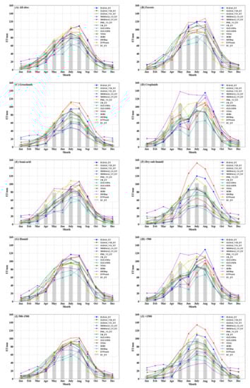
Figure 3.
Comparisons of the monthly average ET values between the eddy covariance (EC) flux tower observations and the different ET products over (A) all EC flux sites, different climatic zones ((B) semiarid, (C) dry subhumid and (D) humid), different land cover types ((E) forests, (F) grasslands and (G) croplands) and different elevations ((H) <500 m, (I) 500 m–1500 m, and (J) >1500 m).
4.1.1. Assessment with All Sites’ Monthly ET
In Figure 4, scatter plots showing the different monthly ET products versus the monthly EC ET according to all of the records from all sites are presented. On the basis of ME and RME, only NTSG overestimated ET, while all other products underestimated ET. It is worth noting that every ET product reposted various levels of performance in different ET ranges. The other assessment indicators were calculated and labeled in the upper left corner of each scatter plot for further detailed analysis (same for the following sections). For the correlation coefficient (R), ETWatch had the reported R value at 0.90 against the EC ET and represented the strongest relationship with EC ET, indicating that the monthly ET changes, by all monthly records of ETWatch, corresponded best with the in situ observed situations. Nevertheless, MOD16A2_C6, MOD16A2_C5, SEBS and SSEBop showed a weaker relationship with EC ET, with R values less than 0.70. Referring to Willmott’s index of agreement (d), ETWatch had the highest value at 0.91, which is consistent with the results of the R analysis. Furthermore, MAEs (RMAEs) varied greatly among the different ET products. The maximum value is 25.32 mm/month (47.30%) by SSEBop, the records of which are the most scattered, while the minimum value is 12.87 mm/month (28.62%) in PML_v2. When comparing the MAE (RMAE) values of every ET product, the RMSE (RRMSE) values are generally greater for all ET products. The higher the number of square operations involved in the RMSE calculation, the more strongly the calculated result is related to the larger value, while the smaller value is ignored. Similar to MAE (RMAE), SSEBop and PML_v2 reported the maximum and minimum RMSE (RRMSE) values at 35.51 mm/month (66.32%) and 18.27 mm/month (40.65%), respectively.
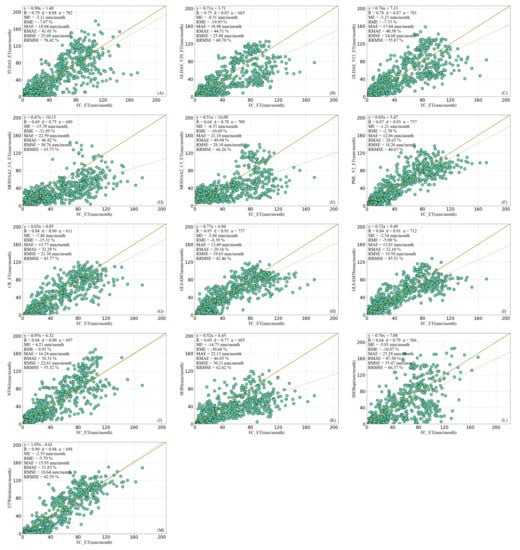
Figure 4.
Monthly values of all ET products ((A) FLDAS_ET; (B) GLDAS_V20_ET (C) GLDAS_V21_ET; (D) MOD16A2_C6_ET; (E) MOD16A2_C5_ET; (F) PML_V2_ET; (G) CR_ET; (H) GLEAM 3.3a; (I) GLEAM 3.3b; (J) NTSG; (K) SEBS; (L) SSEBop and (M) ETWatch) against flux EC ET of all sites’ records.
Figure 5 plots the monthly assessment indicators of the monthly ET products against the monthly EC ET, considering all records from all sites. The patterns of monthly performances of every ET product evaluated with R and d are similar, from which, in general, all products performed relatively better from April to May and from September to October. Interestingly, SSEBop showed a better performance from November to May in terms of R and d, the pattern of which is quite distinct from other ET products. From ME and RME, it can be seen that different ET products are all overestimated or underestimated in different months to varying degrees. For instance, MOD16A2_C5 had a large negative ME from May to September but had the largest positive RME in January and December, meaning that MOD16A2_C5 had the largest positive deviation from EC ET in January and December, in comparison with the other ET products. Evidently, the patterns of monthly performances with MAE (RMAE) and RMSE (RRMSE) also look similar. From the perspectives of MAE and RMSE, MOD16A2_C6, MOD16A2_C5, FLDAS_ET, GLDAS_v20_ET, GLDAS_v21_ET, SEBS and SSEBop did not perform well, compared to other ET products from May to August. The largest MAE and RMSE values were from MOD16A2_C6 and SSEBop. RMAE and RRMSE also shared nearly the same pattern but were quite different from that of MAE and RMSE. The largest RMAE and RRMSE values were reported by MOD16A2_C5 in January and December, which is contributed to by the great overestimation in these two months, as confirmed by ME and RME.
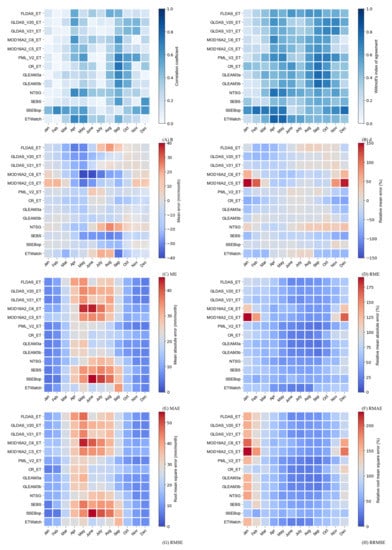
Figure 5.
Monthly assessment indicators ((A) R and (B) d, (C) ME (mm/month), (D) RME (%), (E) MAE (mm/month), (F) RMAE (%), (G) RMSE (mm/month) and (H) RRMSE (%)) of all ET products against the flux EC ET for all site records.
4.1.2. Assessment by Land Cover Type
Figure 6 shows the assessment result by landcover type. According to ME and RME, only MOD16A2_C6, CR_ET and ETWatch were underestimated over forest areas; all ET products were underestimated except for NTSG over grassland areas; and, for cropland areas, only SSEBop was overestimated. The other ET products reported the opposite trends for the three land cover types. Over forest areas, NTSG and SSEBop had the most accurate estimates of ET, with R values greater than 0.93, and the smallest MAE (RMAE) and RMSE (RRMSE) values. PML_v2 reported the highest d value over grassland of 0.94, while PML_v2, GLEAM 3.3a and GLEAM 3.3b reported the highest R value. In addition, the aforementioned three ET products also had the best MAE (RMAE) and RMSE (RRMSE) values. For cropland areas, the most expected R (d) values were from the ETWatch dataset at 0.90 (0.94). Fine MAE and RMSE values were also reported by ETWatch, NTSG, GLEAM 3.3b and PML_v2, in which all MAE values were lower than 20 mm/month and all RMSE values were lower than 25 mm/month.
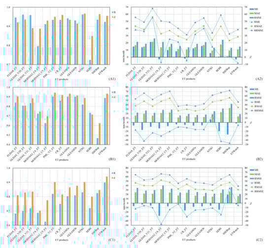
Figure 6.
Summary of the assessment indicators ((1) R and d, (2) ME (mm/month), MAE (mm/month), RMSE (mm/month), RME (%), RMAE (%) and RRMSE (%)) for the monthly ET products against the flux EC ET of different land cover type records ((A) forests, (B) grasslands and (C) croplands).
4.1.3. Assessment by Climatic Zones
Figure 7 illustrates the assessment result by climatic zones. Over semiarid areas, only SSEBop slightly overestimated ET, while other ET products underestimated ET; only NTSG overestimated ET values in the dry subhumid areas; and, in humid areas, MOD16A2_C6, CR_ET, SEBS, SSEBop and ETWatch underestimated ET values. Over semiarid areas, GLDAS_v21_ET, PML_v2, GLEAM 3.3a, GLEAM 3.3b and ETWatch reported R values greater than 0.80 and d values greater than 0.87, while only PML_v2 reported the most desired MAE (RMAE) and RMSE (RRMSE) values. PML_v2 and CR_ET showed the best agreement with the flux EC ET over dry subhumid regions, with high values of R exceeding 0.94, high values of d exceeding 0.95 and relatively low MAE (RMAE) and RMSE (RRMSE) values. Additionally, NTSG and CR_ET outperformed all other ET products over humid areas. Although NTSG had the highest R (d), CR_ET had the smallest MAE (RMAE) and RMSE (RRMSE) values.
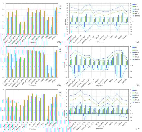
Figure 7.
Summary of the assessment indicators ((1) R and d, (2) ME (mm/month), MAE (mm/month), RMSE (mm/month), RME (%), RMAE (%) and RRMSE (%)) for the monthly ET products against the flux EC ET of different climatic zone records ((A) semiarid, (B) dry subhumid, and (C) humid).
4.1.4. Assessment by Elevation Levels
Figure 8 shows the assessment result by elevation levels. From Figure 8, it can be concluded that only SSEBop overestimated ET over areas with elevations below 500 m. ETWatch had the highest R (d), while GLEAM 3.3b had the smallest MAE (RMAE) and RMSE (RRMSE) values. MOD16A2_C6, CR_ET, SEBS, SSEBop and ETWatch were underestimated over areas with elevations ranging from 500 m to 1500 m. PML_v2 simultaneously had the highest R (d) values and the most expected MAE (RMAE) and RMSE (RRMSE) values, which outperformed all other ET products, in light of all the assessment indicators. All ET products were underestimated over regions with elevations above 1500 m, excluding NTSG. PML_v2 and GLEAM 3.3a had the highest R (d) values, while GLEAM 3.3a had the smallest MAE (RMAE) values, and CR_ET had the smallest RMSE (RRMSE) values.
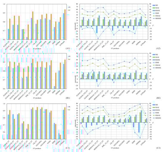
Figure 8.
Summary of the assessment indicators ((1) R and d, (2) ME (mm/month), MAE (mm/month), RMSE (mm/month), RME (%), RMAE (%) and RRMSE (%)) for the monthly ET products against the flux EC ET of the different elevation levels recorded ((A) <500 m, (B) 500–1500 m and (C) >1500 m).
4.2. Overall Assessment Result
In general, the different ET datasets are evaluated based on a constructed two-level assessment sheet, where comparisons among each ET products over different conditions were conducted. There are eight assessment indicators in a row (ME, RME, MAE, RMAE, RMSE, RRMSE, R and d) and 21 assessment conditions in a column, including the 9 aforementioned conditions (land cover types: l01–l03; climatic zones: c01–c03; elevation levels: e01–e03) and individual assessment conditions of interannual months (m01–m12). There are, in total, 168 cells in the assessment sheet. Every cell refers to a process of comparison among every other certain ET product under the column-specified condition, according to the row-specified assessment indicator, and is labeled with the name of the ET product, which has the best performance. To determine the performance of each ET product, lower MAE, RMAE, RMSE and RRMSE values and higher R and d values are expected. Level-1 assessment refers to the selection of the ET product with the highest R and d values and lowest ME, RME, MAE, RMAE, RMSE and RRMSE values, while level-2 assessment aims to select the ET product with the second highest R and d values and the second lowest ME, RME, MAE, RMAE, RMSE and RRMSE values. It is noteworthy that the absolute values of ME and RME are used during the assessment. Next, statistics on the occurrences of the different ET products under each condition (m01–m12, l01–l03, c01–c03 and e01–e03) in the assessment sheet are performed. The number of occurrences and corresponding proportions of all ET products are listed, according to which all ET products were arranged in descending order.
Figure 9 presents the two-level assessment sheet covering all ET products, while Figure 10 presents the comprehensive assessment results. It can be concluded from Figure 10 that PML_V2, ETWatch, GLEAM 3.3a, CR_ET and SSEBop are the five most highly ranked ET products within the level-1 assessment, while PML_V2, GLEAM 3.3a, ETWatch, GLEAM 3.3b and NTSG are ranked in the top five in the level-2 assessment. All of the top five products in the two-level assessment occupy more than 10% of the cells in the assessment sheet. Considering the two-level assessment together, PML_V2, ETWatch, and GLEAM 3.3a, CR_ET and SSEBop are the five best-performing ET products. Together with Figure 10 (ET products are listed in descending order by total counts of cells occupied), detailed descriptions are as follows: PML_V2 occupies 40 (23.81%) and 30 (17.86%) cells, with the highest R and d and lowest ME, RME, MAE, RMAE, RMSE and RRMSE values in level-1 and level-2, respectively. Therefore, there are 70 (20.83%) PML_V2 cells in total in the 2-level assessment. Likewise, the other four highest-performing ET products under all conditions are GLEAM 3.3a (level-1: 25 cells (14.88%); level-2: 26 cells (15.48%); total: 51 cells (15.18%)), ETWatch (level-1: 32 cells (19.05%); level-2: 18 cells (10.71%); total: 50 cells (14.88%)), CR_ET (level-1: 20 cells (11.9%); level-2: 15 cells (8.93%); total: 35 cells (10.42%)) and SSEBop (level-1: 18 cells (10.71%); level-2: 16 cells (9.52%); total: 34 cells (10.12%)). ETWatch and NTSG both occupy 18 cells (10.71%) in the level-2 assessment, but ETWatch outperformed NTSG in the comprehensive two-level assessment and occupies 21 more cells than NTSG.
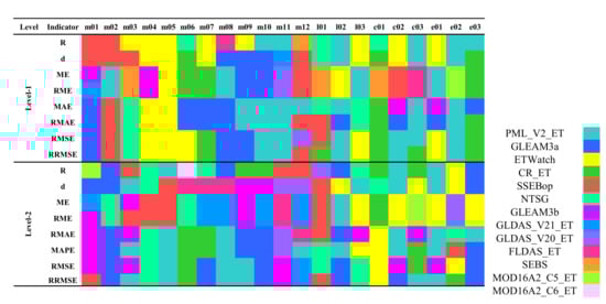
Figure 9.
The 2-level assessment sheet covering all ET products under the conditions of interannual months (January–December: m01–m12), land cover types (forests, grasslands and croplands: l01–l03), climatic zones (semiarid, dry subhumid and humid: c01–c03) and elevation levels (<500 m, 500 m–1500 m, >1500 m: e01–e03).
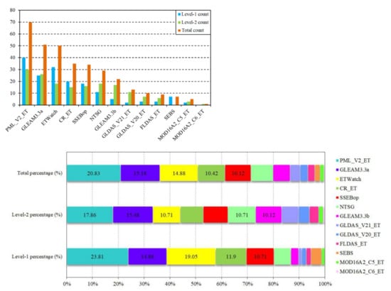
Figure 10.
The count of cells and corresponding percentage of all mentioned ET products with level-1 and level-2 assessments and the total count of cells and their corresponding percentages.
4.3. Synthesis Result
According to the overall assessment result, PML_V2, ETWatch and SSEBop are selected from the top-five ET products for the synthesis dataset from 2003 to 2017, because they had finer spatial resolution from 500 m to 1 km than GLEAM 3.3a and CR_ET. PML_V2 was resampled from 500 m to 1 km with pixel average, while ETWatch and PML_V2 were aggregated to monthly time step from daily and 8-day time steps, respectively. For the synthesis dataset from 1982 to 2002, GLEAM 3.3a, CR_ET and NTSG were selected, because they ranked top-three among the ET products with longer temporal range. The selected three ET products were resampled to 1 km using the nearest neighborhood technique, while GLEAM 3.3a was aggregated to monthly time step. The Taylor skill score of the three selected ET products was calculated with 50% of the in situ measured site month data records (randomly selected for calibration), which were utilized for the determination of their weights for synthesis (Figure 11).
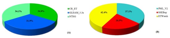
Figure 11.
Weights of three selected ET products calculated with the calibration dataset ((A) 1982–2002, (B) 2003–2017).
Figure 12 shows the multiyear monthly average of the component ET products and the synthesized ET dataset from 2003 to 2017 under the different conditions and observed flux EC ET values. It can be seen from Figure 12 that the monthly average synthesized ET product trend under all conditions is basically consistent with that of EC ET. Generally, the synthesized ET and maximum ET values appear in July, excluding that over forests and humid regions, while the harvesting of winter wheat and sowing of summer maize are well captured from May to July (Figure 12D,H).
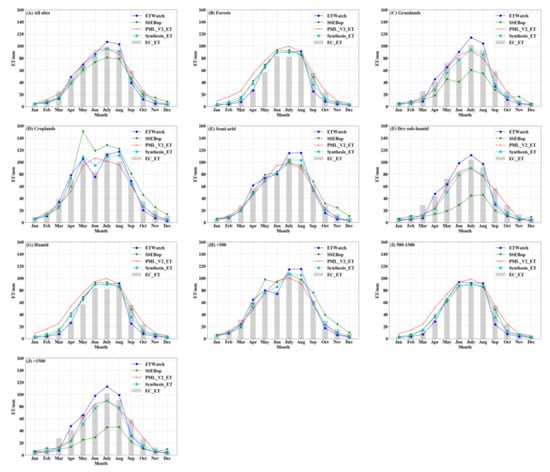
Figure 12.
Comparisons of the monthly average values between the EC flux tower observations, component ET products, and synthesized ET datasets over (A) all EC flux sites, different land cover types ((B) forests, (C) grasslands and (D) croplands), different climatic zones ((E) semiarid, (F) dry subhumid and (G) humid) and different elevation levels ((H) <500 m, (I) 500 m–1500 m and (J) >1500 m).
From the perspective of the average ET from 1982 to 2017 (Figure 13E), the spatial distribution of the synthesized ET of Northern China has obvious regional characteristics and is similar to the "northwest–southeast" belt-like distribution of dry and wet zones divided by multiyear precipitation, where the low-value area (<100 mm) is mainly concentrated in the arid area of the northwest regions, and the high-value area (>500 mm) is mainly concentrated in the eastern monsoon climate regions. Based on the changes in the decadal average ET values (Figure 13A–D), the spatial distribution of the synthesized ET of Northern China is quite consistent, where the low-value areas (<100 mm) only exhibit very minor changes, and the high-value areas (>500 mm) increase to some degree, especially in the plain area of Northern China and Northeast China.
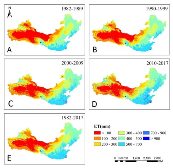
Figure 13.
Spatial distribution of the 5-year average ((A) 1982–1989, (B) 1990–1999, (C) 2000–2009, (D) 2010–2017) and long term ((E) 1982–2017)) synthesized ET datasets.
4.4. Assessment of the Synthesized ET Dataset
The assessment was carried out using the other 50% of the in situ measured EC ET monthly data records as the validation dataset. Figure 14 shows that the synthesized ET agreed well with the observed EC ET data over the interannual months and under the conditions of different land cover types, climatic zones and elevation levels. R was greater than 0.90, while d was greater than 0.95, excluding that of grassland regions, dry subhumid regions and regions with elevation levels >1500 m. Based on ME (RME), the synthesized ET underestimated the flux EC ET under all conditions to varying degrees with no exceptions. The synthesized ET performed best over forested regions, humid regions and regions with elevation levels of <500 m among the different land cover types, climatic zones and elevation levels, respectively, according to the MAE (RMAE) and RMSE (RRMSE) values.
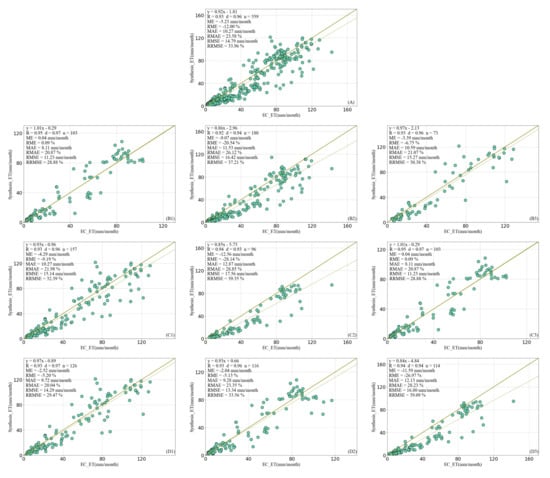
Figure 14.
Monthly average of the synthesized ET products against the flux EC ET of (A) all EC flux sites, different land cover types ((B1) forests, (B2) grasslands and (B3) croplands), different climatic zones ((C1) semiarid, (C2) dry subhumid and (C3) humid) and different elevation levels ((D1) <500 m, (D2) 500 m–1500 m and (D3) >1500 m).
The assessment sheet method was applied here for comparison among the component ET products (PML_V2_ET, ETWatch and SSEBop) and the synthesized results from 2003 to 2017. Figure 15 presents a summary of the assessment sheet. It is obvious that the synthesis result occupied most of the cells in the two-level assessment sheet, showing comprehensive advantages over all other component ET products.
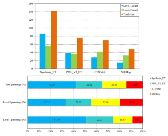
Figure 15.
Count of cells and corresponding percentages of component ET products and the synthesized results with level-1 and level-2 assessment and the total counts of the cells and their corresponding percentages.
Heihe River Basin, a closed inland river basin without outflows in the arid region of northwestern China, is chosen here to conduct water balance assessment for the comparison among component ET products (GLEAM v3.3a, NTSG and CR_ET) and the synthesized results from 1982 to 2002. As mentioned above, the annual mean ET can be approximately regarded as equal to the mean annual precipitation, because there’s no runoff exchange between the closed Heihe River Basin and adjacent regions. Though there are some limitations without considering factors like soil moisture and irrigation, it is still utilized in some closed river basins [49]. Table 4 presents the summary of the results of the water balance assessment. The annual precipitation ranges from 113.2 to 172.9 mm, covering the period from 1982 to 2002, and the mean annual precipitation is 142.7 mm. The mean annual synthesis ET from 1982 to 2002 is 136.3 mm, with −4.0% of the bias to mean annual precipitation. As for component ET products, NTSG, CR_ET and GLEAM v3.3a have a bias of 6.5%, 8.3% and −25.3%, respectively. It’s obvious that synthesis ET outperformed the three component ET products.
Table 4.
Annual precipitation, synthesis ET and component ET (in mm) with corresponding bias to precipitation (in %) from 1982 to 2002 in Heihe River Basin.
5. Discussion
As described in the introduction, acquiring the spatial and temporal characteristics of land surface ET is of vital significance to addressing water resource security and food security issues in Northern China. There have been many global and regional ET products covering Northern China developed using different mechanisms with remote sensing-based models, land surface models (LSMs) and hydrological models with differing model inputs, parameterizations and algorithms and varied spatiotemporal resolutions and temporal ranges. To date, no single ET product can provide relatively accurate long-term ET estimations at a fine spatial resolution. Therefore, this study utilized a two-level assessment scheme to select the best-performing ET products with relatively high spatial resolutions; we presented a synthesized ET dataset with a 1 km spatial resolution covering the period ranging from 1982 to 2017 with the weighted mean of the selected ET products, which can be used directly in relevant studies for Northern China.
When referring to the assessment, the in situ measured ET from EC tower observations was used to carry out the assessment at a site-pixel scale for every selected ET product and aimed to select the optimal ET products with which to build a long-term synthesized ET dataset. Then, a two-level assessment sheet with eight indicators under 21 conditions was built, and statistics describing the different ET product occurrences and corresponding ratios were calculated to select high-resolution ET products with optimal performances. Regarding the overall assessment result, only NTSG overestimated EC ET, while other ET products all underestimated EC ET. For NTSG, the generally overestimated net radiation was the main causes of uncertainties in the estimation of ET [7]. Several ET products had relatively larger deviation to EC ET. The severe underestimation of MOD16 ET products was found across all types of the underlying surface except cropland [87], the reason of which might be attributed to structural characteristics of underlying surfaces and surface conductance parameterizations. The LSM based ET products also showed relative larger deviation to EC ET mainly due to the reanalysis driving data, which was reported to have lower accuracy than satellite driven products [88]. In addition, the uncertainties of SEBS was caused by the situation of the heat transfer simulation within the roughness sublayer (RSL), which often occurs over heterogeneous underlying surfaces like forest [89].
Observations from heterogeneously distributed flux EC sites are a preferable reference for obtaining accurate ET estimations regionally. Even though are limited flux sites in Northern China, this sort of exercise can still contribute to the knowledge of different ET product performances. Though there is still a certain deficiency of in situ EC ET measurements, such as the limited spatial representativeness and the issue of energy balance closure [90,91,92], it is still the most common way to describe the flux exchange occurring between the surface and atmosphere [93] and is still implemented in various relevant studies for the assessment of ET estimations at a site–pixel scale [10,62,68].
After the selection of ET products, the Taylor skill score (TSS) of each ET product was calculated to determine their relative weights. Then, the weighted mean was treated as the synthesis result. Recently, Elnashar et al. [94,95] generated a global synthesis ET product using a simple mean method with an assessment scheme that considered six indicators under 26 conditions. The simple mean of the selected ET products in this research and the aforementioned global synthesis ET product, together with the TSS-based weighted mean results, were assessed with the assessment sheet method using the validation dataset (from 2003 to 2017) and water balance method in Heihe River Basin (from 1982 to 2002), as mentioned in Section 4.4, and the results are as follows (Figure 16 and Table 5).
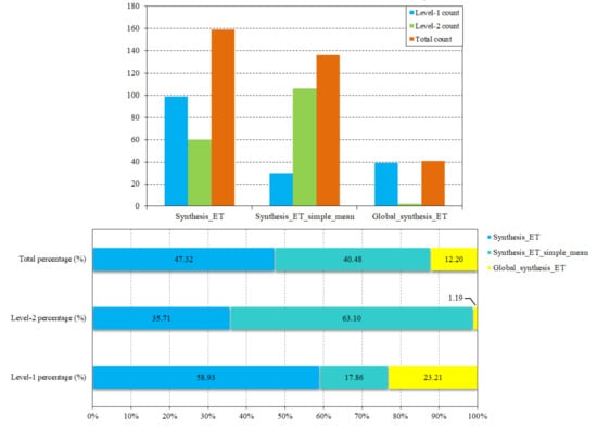
Figure 16.
Count of cells and corresponding percentages of the simple mean of the selected three ET products and the global synthesis ET product generated by Elnashar et al. [94,95]. The weighted mean results in this research with level-1 and level-2 assessment and the total count of cells and their corresponding percentages are shown here.
Table 5.
The simple mean of the selected three ET products and the global synthesis ET product generated by Elnashar et al. [94,95], and the weighted mean results in this research (from 1982 to 2002, in mm) with corresponding bias to precipitation (in %) from 1982 to 2002 in Heihe River Basin.
From Figure 16, it can be inferred that the simple mean and weighted mean of the three selected ET products generally outperformed the global synthesis ET product from 2003 to 2017. The weighted mean result had the best performance in the total count (percentage) of cells in the assessment sheet, but the simple mean had a better performance as determined by the level-2 assessment, indicating that the simple mean method had some advantages. The weighted mean method utilized TSS-based weights to ensure more contributions from the better-performing ET products to the synthesis result, which makes it a better choice than the simple mean method. From Table 5, the simple mean slightly outperformed the weighted mean by 0.5% of the bias and substantially outperformed the global synthesis ET product from 1982 to 2017. The performance of the simple mean and weighted mean are very close, because the TSS-based weights of the three selected ET products are very close to each other. In reference to the global synthesis ET product, the component ET products of the synthesis result were selected by global assessment with worldwide flux observation datasets, while the assessment process in this research was implemented locally, which reflected the local performance of each ET product in Northern China.
The most notable contribution of this study is that it was able to prospectively produce a relatively long-term synthesized ET dataset for Northern China with a fine spatial resolution and relatively low uncertainties; additionally, the synthesized ET dataset performed well against the flux EC ET measurements and using water balance method for assessment. This synthesized ET dataset for Northern China provided ET estimations for tested underlying surfaces. Therefore, this synthesized ET dataset has the potential to support regional studies in Northern China over longer temporal periods.
Since different ET products have varying data availabilities, the synthesis ET dataset was built with six individual ET products. Furthermore, the raw spatial resolution of the component ET datasets before 2003 is originally coarse and resampled to 1 km with the nearest neighborhood technique to ensure the consistency with the synthesis dataset from 2003 to 2017. Considering the abovementioned, further study needs more focus on harmonizing the synthesized results of different periods for the improvements of the coherence among pixels. Furthermore, there are no flux observation datasets accessible before 2003; the method proposed in this research would be inapplicable if the synthesis products were required to cover a longer period. Summarizing the abovementioned points, further study on the synthesis method needs to first consider ET products with coarse and fine spatial resolutions. Then, assessment methods of ET products without in situ EC ET measurements should be considered, such as the triple-colocation (TC) method [96] or extended triple-colocation (ETC) method [97]. The uncertainties of certain datasets can be calculated through such methods, while the weights of the datasets for synthesis are inversely proportional to the uncertainty value. The possibilities of applying TC or ETC methods to synthesize ET products with higher spatial resolutions should be further explored.
6. Conclusions
This study provided an effective method for assessing ET products with in situ measured flux EC ET across different months and various underlying surface types to develop a long-term synthesis ET dataset for Northern China. The comprehensive assessment was carried out under different conditions, namely, over interannual months and across different land cover types, climatic zones and elevation levels, and the latter three conditions were stratified into three classes. With the implementation of eight assessment indicators (R, d, ME, RME, MAE, RMAE, RMSE, RRMSE), the ET products that performed best were selected to generate the synthesis ET dataset over different time ranges. It was demonstrated that the PML_V2, ETWatch, GLEAM 3.3a, CR_ET and SSEBop ET products showed the best performance throughout the assessments together, with the consideration of their spatial resolutions and temporal ranges. No single ET product is likely to perform best under all assessment indicators in all conditions, so this study built the synthesis ET dataset from 2003 to 2017 with the weighted mean of the selected high-resolution PML_V2, ETWatch and SSEBop dataset, and the synthesis ET dataset from 1982 to 2002 with the weighted mean of the selected GLEAM 3.3a, CR_ET and NTSG, which had a higher agreement with and a lower deviation from the in situ measured flux EC ET under all conditions. The weights were determined from the Taylor skill score calculated with the ET product and flux EC ET. Moreover, the ensemble ET estimations from 2003 to 2017 over all types of underlying surfaces performed well when compared with the in situ measured flux EC ET, while the ensemble ET estimations from 1982 to 2002 performed well using the water balance method in Heihe River Basin.
The assessment results over interannual months and across every land cover type, climatic zone and elevation level produced information regarding the performance of ET products under different conditions present in Northern China. Overall, the ET synthesis product proposed in this study improved the accuracy of ET estimations to some extent in Northern China, which can be conducive to relevant hydrological, ecological and agricultural research areas.
Author Contributions
L.W. was responsible for manuscript preparation and data processing and presentation. L.W. and A.E. were responsible for the experimental design. B.W. contributed to the conceptual design, manuscript review, funding motivation and project administration. N.Y., W.Z. and H.Z. contributed to the data processing and manuscript review. All authors have read and agreed to the published version of the manuscript.
Funding
This research was financially supported by the National Natural Science Foundation of China (Grant No: 41991232) and Advanced Science Foundation Research Programme of the Chinese Academy of Sciences (Grant No: QYZDY-SSW-DQC014).
Data Availability Statement
The synthesized ET dataset for Northern China is available at https://doi.org/10.7910/DVN/G5BST8 (last access: 10 March 2021).
Acknowledgments
The authors express their gratitude to the data providers that have been used in this study. Special thanks go to the staff members of the Python Software Foundation, Google Earth Engine, and Google Colaboratory. Special thanks also go to the reviewers and editors; your suggestions and efforts significantly enhanced the quality of the paper.
Conflicts of Interest
The authors declare that they have no conflict of interest.
References
- Jung, M.; Reichstein, M.; Ciais, P.; Seneviratne, S.I.; Sheffield, J.; Goulden, M.L.; Bonan, G.; Cescatti, A.; Chen, J.; De Jeu, R. Recent decline in the global land evapotranspiration trend due to limited moisture supply. Nature 2010, 467, 951–954. [Google Scholar] [CrossRef]
- Scott, R.L.; Biederman, J.A. Partitioning evapotranspiration using long-term carbon dioxide and water vapor fluxes. Geophys. Res. Lett. 2017, 44, 6833–6840. [Google Scholar] [CrossRef]
- Mccoll, K.A. Practical and theoretical benefits of an alternative to the Penman-Monteith evapotranspiration equation. Water Resour. Res. 2020, 56. [Google Scholar] [CrossRef]
- Wilson, K.B.; Hanson, P.J.; Mulholland, P.J.; Baldocchi, D.D.; Wullschleger, S.D. A comparison of methods for determining forest evapotranspiration and its components: Sap-flow, soil water budget, eddy covariance and catchment water balance. Agric. For. Meteorol. 2001, 106, 153–168. [Google Scholar] [CrossRef]
- Lawrence, D.M.; Thornton, P.E.; Oleson, K.W.; Bonan, G.B. The partitioning of evapotranspiration into transpiration, soil evaporation, and canopy evaporation in a GCM: Impacts on land–atmosphere interaction. J. Hydrometeorol. 2007, 8, 862–880. [Google Scholar] [CrossRef]
- Jasechko, S.; Sharp, Z.D.; Gibson, J.J.; Birks, S.J.; Yi, Y.; Fawcett, P.J. Terrestrial water fluxes dominated by transpiration. Nature 2013, 496, 347–350. [Google Scholar] [CrossRef]
- Zhang, K.; Kimball, J.S.; Nemani, R.R.; Running, S.W. A continuous satellite-derived global record of land surface evapotranspiration from 1983 to 2006. Water Resour. Res. 2010, 46. [Google Scholar] [CrossRef]
- Liu, W.; Wang, L.; Zhou, J.; Li, Y.; Sun, F.; Fu, G.; Li, X.; Sang, Y.-F. A worldwide evaluation of basin-scale evapotranspiration estimates against the water balance method. J. Hydrol. 2016, 538, 82–95. [Google Scholar] [CrossRef]
- Calanca, P.; Roesch, A.; Jasper, K.; Wild, M. Global warming and the summertime evapotranspiration regime of the Alpine region. Clim. Chang. 2006, 79, 65–78. [Google Scholar] [CrossRef]
- Ruhoff, A.L.; Paz, A.; Aragao, L.; Mu, Q.; Malhi, Y.; Collischonn, W.; Rocha, H.; Running, S.W. Assessment of the MODIS global evapotranspiration algorithm using eddy covariance measurements and hydrological modelling in the Rio Grande basin. Hydrol. Sci. J. 2013, 58, 1658–1676. [Google Scholar] [CrossRef]
- Xue, B.-L.; Wang, L.; Li, X.; Yang, K.; Chen, D.; Sun, L. Evaluation of evapotranspiration estimates for two river basins on the Tibetan Plateau by a water balance method. J. Hydrol. 2013, 492, 290–297. [Google Scholar] [CrossRef]
- Tasumi, M. Estimating evapotranspiration using METRIC model and Landsat data for better understandings of regional hydrology in the western Urmia Lake Basin. Agric. Water Manag. 2019, 226, 105805. [Google Scholar] [CrossRef]
- Walker, E.; García, G.A.; Venturini, V.; Carrasco, A. Regional evapotranspiration estimates using the relative soil moisture ratio derived from SMAP products. Agric. Water Manag. 2019, 216, 254–263. [Google Scholar] [CrossRef]
- Boé, J.; Terray, L. Uncertainties in summer evapotranspiration changes over Europe and implications for regional climate change. Geophys. Res. Lett. 2008, 35. [Google Scholar] [CrossRef]
- Yin, Y.; Wu, S.; Zhao, D.; Zheng, D.; Pan, T. Modeled effects of climate change on actual evapotranspiration in different eco-geographical regions in the Tibetan Plateau. J. Geogr. Sci. 2013, 23, 195–207. [Google Scholar] [CrossRef]
- Pan, S.; Tian, H.; Dangal, S.R.; Yang, Q.; Yang, J.; Lu, C.; Tao, B.; Ren, W.; Ouyang, Z. Responses of global terrestrial evapotranspiration to climate change and increasing atmospheric CO2 in the 21st century. Earths Future 2015, 3, 15–35. [Google Scholar] [CrossRef]
- Dong, Q.; Wang, W.; Shao, Q.; Xing, W.; Ding, Y.; Fu, J. The response of reference evapotranspiration to climate change in Xinjiang, China: Historical changes, driving forces, and future projections. Int. J. Climatol. 2020, 40. [Google Scholar] [CrossRef]
- Anderson, M.C.; Kustas, W.P. Mapping Evapotranspiration and Drought at local to Continental Scales using Thermal Remote Sensing. In Proceedings of the IEEE International Geoscience & Remote Sensing Symposium, Boston, MA, USA, 7–11 July 2008. [Google Scholar]
- Yao, Y.; Liang, S.; Qin, Q.; Wang, K.; Zhao, S. Monitoring global land surface drought based on a hybrid evapotranspiration model. Int. J. Appl. Earth Obs. Geoinf. 2011, 13, 447–457. [Google Scholar] [CrossRef]
- Antofie, T.; Vogt, J.; Sepulcre-Canto, G.; Arboleda, A. Assessment of the EUMETSAT LSA-SAF evapotranspiration product for drought monitoring in Europe. Int. J. Appl. Earth Obs. Geoinf. 2014. [Google Scholar] [CrossRef]
- Morse, A. Satellite-Based Evapotranspiration by Energy Balance for Western States Water Management. In Proceedings of the Impacts of Global Climate Change, Anchorage, AK, USA, 15–19 May 2005. [Google Scholar]
- Hochmuth, H.; Thevs, N.; He, P. Water allocation and water consumption of irrigation agriculture and natural vegetation in the Heihe River watershed, NW China. Environ. Earth Sci. 2015, 73, 5269–5279. [Google Scholar] [CrossRef]
- Wu, B.; Zeng, H.; Yan, N.; Zhang, M. Approach for Estimating Available Consumable Water for Human Activities in a River Basin. Water Resour. Manag. 2018, 32, 2353–2368. [Google Scholar] [CrossRef]
- Mahmoud, S.H.; Yew, G.T. Irrigation water management in arid regions of Middle East: Assessing spatio-temporal variation of actual evapotranspiration through remote sensing techniques and meteorological data. Agric. Water Manag. 2019, 212, 35–47. [Google Scholar] [CrossRef]
- Davis, S.L.; Dukes, M.D. Irrigation scheduling performance by evapotranspiration-based controllers. Agric. Water Manag. 2010, 98, 19–28. [Google Scholar] [CrossRef]
- Huang, W.C.; Lee, J.L.; Tsai, A.Y. Impact of Evapotranspiration on Agricultural Water Resources under Climate Change. In Proceedings of the 2012 2nd International Conference on Environmental and Agriculture Engineering, Jeju Island, Korea, 29 June 2012. [Google Scholar]
- Baik, J.; Choi, M. Agricultural Water Management Evaluation of geostationary satellite (COMS) based Priestley–Taylor evapotranspiration. Agric. Water Manag. 2015, 159, 77–91. [Google Scholar] [CrossRef]
- Jamshidi, S.; Zand-Parsa, S.; Kamgar-Haghighi, A.A.; Shahsavar, A.R.; Niyogi, D. Evapotranspiration, crop coefficients, and physiological responses of citrus trees in semi-arid climatic conditions. Agric. Water Manag. 2020, 227. [Google Scholar] [CrossRef]
- Han, B.F.; Liu, Y.B. Impacts of different ecological restoration measurements on the evapotranspiration characteristics of the typical steppe in the loess hilly area of Ningixa. J. Agric. Sci. 2013, 4, 7–10. [Google Scholar]
- Lu, K.; Garcia, M.; Yu, J.; Zhang, Y.; Ping, W.; Sheng, W.; Xiao, L. Ecological restoration of groundwater-dependent vegetation in the arid Ejina Delta: Evidences from satellite evapotranspiration. In Proceedings of the 19th EGU General Assembly, EGU2017, Vienna, Austria, 23–28 April 2017. [Google Scholar]
- Scott, S.; Si, Z.; Schumilas, T.; Chen, A. Organic Food and Farming in China: Top-Down and Bottom-Up Ecological Initiatives; Routledge: Abingdon, UK, 2018. [Google Scholar]
- Qiu, G.Y.; Jin, Y.; Geng, S. Impact of Climate and Land-Use Changes on Water Security for Agriculture in Northern China. J. Integr. Agric. 2012, 11, 144–150. [Google Scholar] [CrossRef]
- Oki, T.; Kanae, S.; Musiake, K. Global Hydrological Cycles and World Water Resources. Science 2006, 313, 1068–1072. [Google Scholar] [CrossRef] [PubMed]
- Bowen, I.S. The Ratio of Heat Losses by Conduction and by Evaporation from any Water Surface. Phys. Rev. 1926, 27, 779. [Google Scholar] [CrossRef]
- Monteith, J.; Unsworth, M. Principles of Environmental Physics, 4th ed.; Elsevier: Amsterdam, The Netherlands, 2008. [Google Scholar]
- Allen, R.G. Lysimeters for evapotranspiration and environmental measurements. In Proceedings of the International Symposium on Lysimetry, Honolulu, HI, USA, 23–25 July 1991. [Google Scholar]
- Ran, Y.; Li, X.; Kljun, N.; Sun, R.; Zhang, L. Spatial Representativeness and Uncertainty of Eddy Covariance Carbon Flux Measurement for Upscaling Net Ecosystem Productivity to Field Scale. In Proceedings of the Agu Fall Meeting, San Francisco, CA, USA, 14–18 December 2015. [Google Scholar]
- Herman, M.R.; Nejadhashemi, A.P.; Abouali, M.; Hernandez-Suarez, J.S.; Daneshvar, F.; Zhang, Z.; Anderson, M.C.; Sadeghi, A.M.; Hain, C.R.; Sharifi, A. Evaluating the role of evapotranspiration remote sensing data in improving hydrological modeling predictability. J. Hydrol. 2018, 556, 39–49. [Google Scholar] [CrossRef]
- Li, Z.-L.; Tang, R.; Wan, Z.; Bi, Y.; Zhou, C.; Tang, B.; Yan, G.; Zhang, X. A Review of Current Methodologies for Regional Evapotranspiration Estimation from Remotely Sensed Data. Sensors 2009, 9, 3801–3853. [Google Scholar] [CrossRef] [PubMed]
- Zhang, Y.; Kong, D.; Gan, R.; Chiew, F.H.S.; McVicar, T.R.; Zhang, Q.; Yang, Y. Coupled estimation of 500m and 8-day resolution global evapotranspiration and gross primary production in 2002–2017. Remote Sens. Environ. 2019, 222, 165–182. [Google Scholar] [CrossRef]
- Chen, X.; Su, Z.; Ma, Y.; Yang, K.; Wen, J.; Zhang, Y. An Improvement of Roughness Height Parameterization of the Surface Energy Balance System (SEBS) over the Tibetan Plateau. J. Appl. Meteorol. Climatol. 2013, 52, 607–622. [Google Scholar] [CrossRef]
- Senay, G.B.; Bohms, S.; Singh, R.K.; Gowda, P.H.; Velpuri, N.M.; Alemu, H.; Verdin, J.P. Operational evapotranspiration mapping using remote sensing and weather datasets: A new parameterization for the SSEB approach. J. Am. Water Resour. Assoc. 2013, 49, 577–591. [Google Scholar] [CrossRef]
- Mu, Q.; Zhao, M.; Running, S.W. Improvements to a MODIS global terrestrial evapotranspiration algorithm. Remote Sens. Environ. 2011, 115, 1781–1800. [Google Scholar] [CrossRef]
- Cosgrove, B.A. Land surface model spin-up behavior in the North American Land Data Assimilation System (NLDAS). J. Geophys. Res. 2003, 108, 8845. [Google Scholar] [CrossRef]
- Miralles, D.G.; Holmes, T.R.H.; De Jeu, R.A.M.; Gash, J.H.; Meesters, A.G.C.A.; Dolman, A.J. Global land-surface evaporation estimated from satellite-based observations. Hydrol. Earth Syst. Sci. 2011, 15, 453–469. [Google Scholar] [CrossRef]
- Rodell, M.; Houser, P.R.; Jambor, U.; Gottschalck, J.; Mitchell, K.; Meng, C.-J.; Arsenault, K.; Cosgrove, B.; Radakovich, J.; Bosilovich, M.; et al. The Global Land Data Assimilation System. Bull. Am. Meteorol. Soc. 2004, 85, 381–394. [Google Scholar] [CrossRef]
- McNally, A.; Arsenault, K.; Kumar, S.; Shukla, S.; Peterson, P.; Wang, S.; Funk, C.; Peters-Lidard, C.D.; Verdin, J.P. A land data assimilation system for sub-Saharan Africa food and water security applications. Sci. Data 2017, 4, 170012. [Google Scholar] [CrossRef] [PubMed]
- Abatzoglou, J.T.; Dobrowski, S.Z.; Parks, S.A.; Hegewisch, K.C. TerraClimate, a high-resolution global dataset of monthly climate and climatic water balance from 1958–2015. Sci. Data 2018, 5, 170191. [Google Scholar] [CrossRef]
- Wu, B.; Zhu, W.; Yan, N.; Xing, Q.; Wang, L. Regional Actual Evapotranspiration Estimation with Land and Meteorological Variables Derived from Multi-Source Satellite Data. Remote Sens. 2020, 12, 332. [Google Scholar] [CrossRef]
- Ma, N.; Szilagyi, J.; Zhang, Y.; Liu, W. Complementary-Relationship-Based Modeling of Terrestrial Evapotranspiration Across China During 1982–2012: Validations and Spatiotemporal Analyses. J. Geophys. Res. Atmos. 2019, 124, 4326–4351. [Google Scholar] [CrossRef]
- Chen, M.; Senay, G.B.; Verdin, J.P.; Rowland, J. Uncertainty Analysis on an Operational Simplified Surface Energy Balance algorithm for Estimation of Evapotranspiration at Multiple Flux Tower Sites. In Proceedings of the Agu Fall Meeting, San Francisco, CA, USA, 15–19 December 2014. [Google Scholar]
- Nearing, G.S.; Mocko, D.M.; Peters-Lidard, C.D.; Kumar, S.V.; Xia, Y. Benchmarking NLDAS-2 Soil Moisture and Evapotranspiration to Separate Uncertainty Contributions. J. Hydrometeorol. 2016, 17, 745–759. [Google Scholar] [CrossRef] [PubMed]
- Jin, X.M.; Li, W.; Liang, J.Y. Accuracy Verification of Evapotranspiration Result Using Hydrological Budget Method—A Case Study of the Zhangye Basin. Geoscience 2008, 2, 159–163. [Google Scholar]
- Leuning, R.; Zhang, Y.Q.; Rajaud, A.; Cleugh, H.; Tu, K. A simple surface conductance model to estimate regional evaporation using MODIS leaf area index and the Penman-Monteith equation. Water Resour. Res. 2008, 44, 652–655. [Google Scholar] [CrossRef]
- Allen, R.G.; Pereira, L.S.; Howell, T.A.; Jensen, M.E. Evapotranspiration information reporting: I. Factors governing measurement accuracy. Agric. Water Manag. 2011, 98, 899–920. [Google Scholar] [CrossRef]
- Kim, H.W.; Hwang, K.; Mu, Q.; Lee, S.O.; Choi, M. Validation of MODIS 16 global terrestrial evapotranspiration products in various climates and land cover types in Asia. KSCE J. Civ. Eng. 2012, 16, 229–238. [Google Scholar] [CrossRef]
- Wang, K.; Dickinson, R.E. A review of global terrestrial evapotranspiration: Observation, modeling, climatology, and climatic variability. Rev. Geophys. 2012, 50. [Google Scholar] [CrossRef]
- Hu, G.; Jia, L.; Menenti, M. Comparison of MOD16 and LSA-SAF MSG evapotranspiration products over Europe for 2011. Remote Sens. Environ. 2015, 156, 510–526. [Google Scholar] [CrossRef]
- Wu, B.F.; Xiong, J.; Yan, N.N.; Yang, L.D.; Du, X. ETWatch for monitoring regional evapotranspiration with remote sensing. Adv. Water Sci. 2008, 19, 671–678. [Google Scholar]
- Wu, B.; Yan, N.; Xiong, J.; Bastiaanssen, W.G.M.; Zhu, W.; Stein, A. Validation of ETWatch using field measurements at diverse landscapes: A case study in Hai Basin of China. J. Hydrol. 2012, 436, 67–80. [Google Scholar] [CrossRef]
- Vinukollu, R.K.; Meynadier, R.; Sheffield, J.; Wood, E.F. Multi-model, multi-sensor estimates of global evapotranspiration: Climatology, uncertainties and trends. Hydrol. Process. 2011, 25, 3993–4010. [Google Scholar] [CrossRef]
- Ershadi, A.; McCabe, M.F.; Evans, J.P.; Chaney, N.W.; Wood, E.F. Multi-site evaluation of terrestrial evaporation models using FLUXNET data. Agric. For. Meteorol. 2014, 187, 46–61. [Google Scholar] [CrossRef]
- Chen, Y.; Yuan, W.; Xia, J.; Fisher, J.B.; Dong, W.; Zhang, X.; Liang, S.; Ye, A.; Cai, W.; Feng, J. Using Bayesian model averaging to estimate terrestrial evapotranspiration in China. J. Hydrol. 2015, 528, 537–549. [Google Scholar] [CrossRef]
- Zhu, G.; Li, X.; Zhang, K.; Ding, Z.; Han, T.; Ma, J.; Huang, C.; He, J.; Ma, T. Multi-model ensemble prediction of terrestrial evapotranspiration across north China using Bayesian model averaging. Hydrol. Process. 2016, 30, 2861–2879. [Google Scholar] [CrossRef]
- Yao, Y.; Liang, S.; Li, X.; Zhang, Y.; Chen, J.; Jia, K.; Zhang, X.; Fisher, J.B.; Wang, X.; Zhang, L. Estimation of high-resolution terrestrial evapotranspiration from Landsat data using a simple Taylor skill fusion method. J. Hydrol. 2017, 553, 508–526. [Google Scholar] [CrossRef]
- Baik, J.; Liaqat, U.W.; Choi, M. Assessment of satellite-and reanalysis-based evapotranspiration products with two blending approaches over the complex landscapes and climates of Australia. Agric. For. Meteorol. 2018, 263, 388–398. [Google Scholar] [CrossRef]
- Niyogi, D.; Jamshidi, S.; Smith, D.; Kellner, O. Evapotranspiration Climatology of Indiana, USA Using In-Situ and Remotely Sensed Products. J. Appl. Meteorol. Climatol. 2020, 59, 2093–2111. [Google Scholar] [CrossRef]
- Mueller, B.; Hirschi, M.; Jimenez, C.; Ciais, P.; Dirmeyer, P.A.; Dolman, A.J.; Fisher, J.B.; Jung, M.; Ludwig, F.; Maignan, F.; et al. Benchmark products for land evapotranspiration: LandFlux-EVAL multi-data set synthesis. Hydrol. Earth Syst. Sci. 2013, 17, 3707–3720. [Google Scholar] [CrossRef]
- Badgley, G.; Fisher, J.B.; Jiménez, C.; Tu, K.P.; Vinukollu, R. On Uncertainty in Global Terrestrial Evapotranspiration Estimates from Choice of Input Forcing Datasets. J. Hydrometeorol. 2015, 16, 1449–1455. [Google Scholar] [CrossRef]
- Jiang, S.; Wei, L.; Ren, L.; Xu, C.Y.; Liu, Y. Utility of integrated IMERG precipitation and GLEAM potential evapotranspiration products for drought monitoring over mainland China. Atmos. Res. 2020, 247, 105141. [Google Scholar] [CrossRef]
- Reichstein, M.; Falge, E.; Baldocchi, D.; Papale, D.; Aubinet, M.; Berbigier, P.; Bernhofer, C.; Buchmann, N.; Gilmanov, T.; Granier, A. On the separation of net ecosystem exchange into assimilation and ecosystem respiration: Review and improved algorithm. Glob. Chang. Biol. 2005, 11, 1424–1439. [Google Scholar] [CrossRef]
- Su, Z. The surface energy balance system (SEBS) for estimation of turbulent heat fluxes. Hydrol. Earth Syst. Sci. 2002, 6, 85–99. [Google Scholar] [CrossRef]
- Walter, I.A.; Allen, R.G.; Elliott, R.; Jensen, M.; Itenfisu, D.; Mecham, B.; Howell, T.; Snyder, R.; Brown, P.; Echings, S. ASCE’s standardized reference evapotranspiration equation. In Watershed Management and Operations Management 2000; American Society of Civil Engineers: Fort Collins, CO, USA, 2000; pp. 1–11. [Google Scholar]
- Henderson-Sellers, B. A new formula for latent heat of vaporization of water as a function of temperature. Q. J. R. Meteorol. Soc. 1984, 110, 1186–1190. [Google Scholar] [CrossRef]
- Li, S.; Wang, G.; Sun, S.; Chen, H.; Bai, P.; Zhou, S.; Huang, Y.; Wang, J.; Deng, P. Assessment of Multi-Source Evapotranspiration Products over China Using Eddy Covariance Observations. Remote Sens. 2018, 10, 1692. [Google Scholar] [CrossRef]
- Farr, T.G.; Rosen, P.A.; Caro, E.; Crippen, R.; Duren, R.; Hensley, S.; Kobrick, M.; Paller, M.; Rodriguez, E.; Roth, L.; et al. The Shuttle Radar Topography Mission. Rev. Geophys. 2007, 45. [Google Scholar] [CrossRef]
- Zomer, R.J.; Trabucco, A.; Bossio, D.A.; Verchot, L.V. Climate change mitigation: A spatial analysis of global land suitability for clean development mechanism afforestation and reforestation. Agric. Ecosyst. Environ. 2008, 126, 67–80. [Google Scholar] [CrossRef]
- Zhao, Y.; Zhu, J.; Xu, Y. Establishment and assessment of the grid precipitation datasets in China for recent 50 years. J. Meteorol. Sci. 2014, 34, 414–420. [Google Scholar]
- Mohammadi, A.; Costelloe, J.F.; Ryu, D. Evaluation of remotely sensed evapotranspiration products in a large scale Australian arid region: Cooper Creek, Queensland. In Proceedings of the International Congress on Modelling & Simulation, Gold Coast, Australia, 29 November–4 December 2015. [Google Scholar]
- McCabe, M.F.; Ershadi, A.; Jimenez, C.; Miralles, D.G.; Michel, D.; Wood, E.F. The GEWEX LandFlux project: Evaluation of model evaporation using tower-based and globally gridded forcing data. Geosci. Model Dev. 2016, 9, 283–305. [Google Scholar] [CrossRef]
- Rim, C.S. A comparison of approaches for evapotranspiration estimation. KSCE J. Civ. Eng. 2000, 4, 47–52. [Google Scholar] [CrossRef]
- Verstraeten, W.W.; Veroustraete, F.; Feyen, J. Estimating evapotranspiration of European forests from NOAA-imagery at satellite overpass time: Towards an operational processing chain for integrated optical and thermal sensor data products. Remote Sens. Environ. 2005, 96, 256–276. [Google Scholar] [CrossRef]
- Xiong, Y.J.; Zhao, W.L.; Wang, P.; Paw U, K.T.; Qiu, G.Y. Simple and Applicable Method for Estimating Evapotranspiration and Its Components in Arid Regions. J. Geophys. Res. Atmos. 2019, 124. [Google Scholar] [CrossRef]
- Bogawski, P.; Bednorz, E. Comparison and validation of selected evapotranspiration models for conditions in Poland (Central Europe). Water Resour. Manag. 2014, 28, 5021–5038. [Google Scholar] [CrossRef]
- UNEP. World Atlas of Desertification; United Nations Environment Programme: Nairobi, Kenya, 1997. [Google Scholar]
- Taylor, K.E. Summarizing multiple aspects of model performance in a single diagram. J. Geophys. Res. 2001, 106, 7183–7192. [Google Scholar] [CrossRef]
- Ershadi, A.; Mccabe, M.F.; Evans, J.P.; Wood, E.F. Impact of model structure and parameterization on Penman–Monteith type evaporation models. J. Hydrol. 2015, 525. [Google Scholar] [CrossRef]
- Jia, B.; Xie, Z.; Dai, A.; Shi, C.; Chen, F. Evaluation of satellite and reanalysis products of downward surface solar radiation over East Asia: Spatial and seasonal variations. J. Geophys. Res. Atmos. 2013, 118, 3431–3446. [Google Scholar] [CrossRef]
- Harman, I.N. The role of roughness sublayer dynamics within surface exchange schemes. Bound. Layer Meteorol. 2012, 142, 1–20. [Google Scholar] [CrossRef]
- Steinfeld, G.; Letzel, M.O.; Raasch, S.; Kanda, M.; Inagaki, A. Spatial representativeness of single tower measurements and the imbalance problem with eddy-covariance fluxes: Results of a large-eddy simulation study. Bound. Layer Meteorol. 2007, 123, 77–98. [Google Scholar] [CrossRef]
- Franssen, H.J.H.; Stöckli, R.; Lehner, I.; Rotenberg, E.; Seneviratne, S.I. Energy balance closure of eddy-covariance data: A multisite analysis for European FLUXNET stations. Agric. For. Meteorol. 2010, 150, 1553–1567. [Google Scholar] [CrossRef]
- Liu, S.M.; Xu, Z.W.; Wang, W.Z.; Jia, Z.Z.; Zhu, M.J.; Bai, J.; Wang, J.M. A comparison of eddy-covariance and large aperture scintillometer measurements with respect to the energy balance closure problem. Hydrol. Earth Syst. Sci. 2011, 15, 1291–1306. [Google Scholar] [CrossRef]
- Webb, E.K.; Pearman, G.I.; Leuning, R. Correction of flux measurements for density effects due to heat and water vapour transfer. Q. J. R. Meteorol. Soc. 2010, 106, 85–100. [Google Scholar] [CrossRef]
- Elnashar, A.; Wang, L.; Wu, B.; Zhu, W.; Zeng, H. Synthesis of Global Actual Evapotranspiration from 1982 to 2019, V1 ed.; Harvard Dataverse: Cambridge, MA, USA, 2020. [Google Scholar] [CrossRef]
- Elnashar, A.; Wang, L.; Wu, B.; Zhu, W.; Zeng, H. Synthesis of Global Actual Evapotranspiration from 1982 to 2019. Earth Syst. Sci. Data. 2021, 13, 447–480. [Google Scholar] [CrossRef]
- Fang, H.; Wei, S.; Jiang, C.; Scipal, K. Theoretical uncertainty analysis of global MODIS, CYCLOPES, and GLOBCARBON LAI products using a triple collocation method. Remote Sens. Environ. 2012, 124, 610–621. [Google Scholar] [CrossRef]
- Mccoll, K.A.; Vogelzang, J.; Konings, A.G.; Entekhabi, D.; Piles, M.; Stoffelen, A. Extended triple collocation: Estimating errors and correlation coefficients with respect to an unknown target. Geophys. Res. Lett. 2015, 41, 6229–6236. [Google Scholar] [CrossRef]


Publisher’s Note: MDPI stays neutral with regard to jurisdictional claims in published maps and institutional affiliations. |
© 2021 by the authors. Licensee MDPI, Basel, Switzerland. This article is an open access article distributed under the terms and conditions of the Creative Commons Attribution (CC BY) license (http://creativecommons.org/licenses/by/4.0/).