Abstract
Mapping crop types and land cover in smallholder farming systems in sub-Saharan Africa remains a challenge due to data costs, high cloud cover, and poor temporal resolution of satellite data. With improvement in satellite technology and image processing techniques, there is a potential for integrating data from sensors with different spectral characteristics and temporal resolutions to effectively map crop types and land cover. In our Malawi study area, it is common that there are no cloud-free images available for the entire crop growth season. The goal of this experiment is to produce detailed crop type and land cover maps in agricultural landscapes using the Sentinel-1 (S-1) radar data, Sentinel-2 (S-2) optical data, S-2 and PlanetScope data fusion, and S-1 C2 matrix and S-1 H/α polarimetric decomposition. We evaluated the ability to combine these data to map crop types and land cover in two smallholder farming locations. The random forest algorithm, trained with crop and land cover type data collected in the field, complemented with samples digitized from Google Earth Pro and DigitalGlobe, was used for the classification experiments. The results show that the S-2 and PlanetScope fused image + S-1 covariance (C2) matrix + H/α polarimetric decomposition (an entropy-based decomposition method) fusion outperformed all other image combinations, producing higher overall accuracies (OAs) (>85%) and Kappa coefficients (>0.80). These OAs represent a 13.53% and 11.7% improvement on the Sentinel-2-only (OAs < 80%) experiment for Thimalala and Edundu, respectively. The experiment also provided accurate insights into the distribution of crop and land cover types in the area. The findings suggest that in cloud-dense and resource-poor locations, fusing high temporal resolution radar data with available optical data presents an opportunity for operational mapping of crop types and land cover to support food security and environmental management decision-making.
1. Introduction
Mapping agricultural landscapes to identify crop types, analyze the spatial distribution of crops and cropping systems, and document land cover types in countries in the Global South is critical for guiding agricultural and environmental planning decision-making, especially in areas experiencing rapid climate change and chronic food insecurity. The type of crops and land cover on the landscape contribute to preventing soil degradation and maintaining soil health [1,2,3]. The diversity of crops on the landscape also contributes to weed control on farmlands and yield improvements by reducing the ability of some pests and diseases to propagate and spread [4,5,6]. Further, a diverse landscape that comprises different crop cultivars and varying plant species supports ecosystem services, including pollination and water quality [7]. Smallholder agriculture is responsible for 84% of the 570 million farms worldwide [8], sustains the food needs of about two-thirds of the more than 3 billion rural inhabitants globally [9], and produces one-third of all food consumed worldwide [10,11]. Moreover, the types of crops and their diversity in the landscape reflects nutrition diversity and food security more broadly [12]. Despite the global significance of smallholder agriculture, there are information gaps on the types of crops cultivated and where the crops are grown, with a paucity of crop inventory data. Yet, information on the types and distribution of crops is essential for monitoring crop yield progress, understanding management practices, prioritizing agrarian policies, and guiding environmental management decisions [13,14]. Due to limited government-led efforts, however, the responsibility has been on researchers and scholars to lead the process of mapping crop and land cover types in such complex landscapes. Many governments in sub-Saharan Africa (SSA) are unable to keep up-to-date crop inventory maps because of the limited infrastructure and resources needed to conduct regular field surveys [15]. Additionally, in countries where the government successfully sponsors such data collection efforts, the data are often not collected in real time to guide within-season decision-making. In SSA countries where crop inventories are available, the lack of resources for conducting routine detailed surveys leads to the data being aggregated at the regional or national scale or covering only parts of a given country [16,17].
Remote sensing has emerged as a low-cost near-real-time technique for large scale operational mapping of agricultural landscapes [18,19]. Advancements in data storage and satellite technology have improved crop type and land cover mapping tremendously over the last few decades. In many countries, crop inventory maps are based on such satellite data. For instance, in the United States, the Department of Agriculture, National Agricultural Statistics Service, generates annual Cropland Data Layer using Landsat and other satellite data, while Agriculture and Agri-Food Canada applies synthetic aperture radar (SAR) data for operational crop inventory mapping. The development of image classification algorithms including machine learning, convolutional neural networks, and deep learning has further improved the accuracy of crop type maps at the field scale in many parts of the world [20,21,22]. In resource-poor settings in SSA where climate change is predicted to have more severe impacts, the advancements in satellite remote sensing and algorithms present an opportunity to develop crop type maps as decision support and resilience-building to food insecurity. Wang et al. [23] contend that remote sensing can aid with crop type mapping if field-level ground data are collected using field surveys to train and validate models to help identify crop types. Even with detailed ground truth data, mapping crop types in the context of smallholder agriculture remains complex because farmlands are smaller, farm-level species are more diverse, agricultural practices are more variable, and intercropping and crop rotations are predominant [8,24,25]. These complexities, coupled with the inadequate reference data (such as crop inventories), imply that identifying and mapping crop types using the regular remote sensing classification methods and moderate resolution data may fail to help identify crop types. The improvement in accuracy of spatial data collection devices including Global Positioning System (GPS) devices and some smartphones can be harnessed for large-scale ground truth data collection for mapping accurate crop types and land cover in smallholder farming systems.
Increasingly, the integration of data from remote sensors with different characteristics (e.g., optical and radar) has gained prominence due to their superior ability to separate different crop and land cover classes in heterogeneous landscapes. Previous studies have applied such an integrative approach to improving classification accuracies. For instance, Wang et al. [23] used crowdsourced ground truth data with Sentinel-1 and Sentinel-2 data and applied a deep learning classification technique to identify rice and cotton crops in India. Wang, Azzari, and Lobell [26] used Landsat data to map crop types in the US Midwest. In terms of land cover type mapping, Kaplan and Avdan [27] fused Sentinel-1 and Sentinel-2 data to map wetlands in Turkey while Slagter et al. [28] fused Sentinel-1 and Sentinel-2 data to map wetlands in South Africa. Kannaujiya et al. [29] integrated electrical resistivity tomography and ground-penetrating radar to map landslides in Kunjethi, while Yan et al. [30] integrated Landsat-8 optical data and Sentinel-1A to detect underground coal fires in China. Venter et al. [31] assessed the efficacy of mapping hyperlocal Tair over Oslo in Norway by integrating Sentinel, Landsat, and light detection and ranging (LiDAR) data with crowdsourced Tair measurements.
In this study, the overall goal is to examine how the integration of multitemporal dual-polarized Sentinel-1 SAR data and multispectral Sentinel-2 and PlanetScope optical data can be used for crop type and land cover mapping in complex heterogeneous agricultural landscapes using a machine learning classification algorithm. The objective is to explore the potential of several possible integrations of Sentinel-1 SAR, Sentinel-2 optical, and high-resolution PlanetScope optical data with diverse data processing techniques for accurate mapping of crop types and land cover in a smallholder agricultural system. Specifically, we compare the results of classifying (i) Sentinel-1-only images, (ii) Sentinel-2-only images, (iii) the fusion of Sentinel-2 and PlanetScope images, (iv) Sentinel-2 and PlanetScope fused image + Sentinel-1 C2 matrix, and (v) Sentinel-2 and PlanetScope fused image + Sentinel-1 C2 matrix + H/α polarimetric decomposition image. The experiments did not consider PlanetScope-only analysis because our goal was to use the PlanetScope image to sharpen the Sentinel-2 images which have more bands, including the red edge band that is more useful for identifying the biophysical variables in vegetation [32]. The experiments are focused on two smallholder agricultural landscapes in rural northern Malawi. The hilly topography in the study locations means that cropping types and land cover characteristics tend to vary over short distances. Our final map, therefore, shows crop types and land cover categories and their distribution. Understanding the distribution of crop and land cover types in these two locations will provide a good overview of the agricultural landscape in the entire region since cropping patterns are generally similar.
2. Materials and Methods
2.1. Study Area Description
The study was conducted in the Edundu village area (land area = ~29 km2) with center location of latitude 11°22.545′ S, longitude 33°46.982′ E, and Thimalala village area (land area = ~22 km2) with center location of latitude 11°16.736′ S, longitude 33°50.995′ E, in northern Malawi (Figure 1). A village area comprises several smaller communities predominantly engaged in smallholder agriculture. The study locations are in the Mzimba district in northern Malawi. Soils in the district are moderately fertile, generally medium- to light-textured, mostly sandy-loam and loamy, with moderate to good drainage [33]. The climatic type in the area is semi-humid, with average monthly maximum temperatures ranging from 27 to 33 °C in the summer (November to April), and from 0 to 10 °C during the winter months (May to August). Annual rainfall amounts range from 800 to 1000 mm [34] which, in a good rainy season, makes the area suitable for the cultivation of a wide variety of crops, including cereals, legumes, and tobacco. The main economic activities in the area are subsistence agriculture and commercial tobacco cultivation [33]. As these smallholders predominantly rely upon rainfed agriculture, the growing season coincides with a rainy season that begins in November or December and ends in April. Maize is the most important subsistence crop cultivated in much of Malawi and is often intercropped with soybeans, groundnuts, beans, and pumpkins in the two study locations. In the last few decades, the district has often been impacted by extreme climate events such as floods and droughts, with predictions that these extremes will worsen as global climate change intensifies [33]. Understanding the dominant crop types and land cover and their distribution in the area will facilitate decision-making to build resilience to these current and projected changes in the climate. Dry season farming (dimba gardening) in valleys contributes significantly to household food security and income in the area for households that have access to the wetlands [35]. This research was part of a broader participatory interdisciplinary research project aimed at understanding the relationship between farm management practices, wild biodiversity, and ecosystem services, to develop scenarios for community action plans.
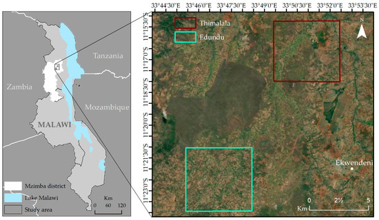
Figure 1.
A general overview of the study area in the northern part of Malawi.
2.2. Data Acquisition
2.2.1. Satellite Data
A combination of radar (Sentinel-1) and optical (Sentinel-2 and PlanetScope) satellite images were used in this study. The sensor specifications of the data used are presented in Table 1. The Sentinel-1 constellation has two satellites—Sentinel-1A and Sentinel-1B, which were launched in April 2014 and April 2016, respectively. Sentinel-1 Single Look Complex (SLC) products, provided by the European Space Agency (ESA), consist of SAR data in the C-band and capture 5–20 m spatial resolution imagery. The two satellites have a combined revisit period of 6 days [36]. SAR images contain coherent (interferometric phases) and incoherent (amplitude features) information. The interferometric wide (IW) swatch mode, which acquires images with dual-polarization (vertical transmit, vertical receive (VV) and vertical transmit, horizontal receive (VH)), was used [36]. Abdikan et al. [37] investigated the efficiency of Sentinel-1 SAR images in land cover mapping over Turkey and found that the dual polarimetric Sentinel-1 SAR data can be used to produce accurate land cover maps. SAR products are mostly used in combination with optical images to improve crop classification accuracy [38] and class discrimination [39] since they are not affected by clouds, haze, and smoke.

Table 1.
Comparison of sensor specifications for Sentinel-1, Sentinel-2, and PlanetScope.
The Sentinel-2 data used in this study were also acquired from the ESA. The Sentinel-2A (launched in June 2015) and 2B (launched in March 2017) satellites have a combined revisit period of 5 days, making them suitable for monitoring crop growth compared to other satellites, such as the Landsat, that have a lower temporal resolution. Both Sentinel-2A and Sentinel-2B satellites carry a single multispectral instrument with 13 spectral bands. We used a top of the atmosphere (TOA) reflectance product (Level-1C) provided freely by the ESA for this study. A higher-level surface reflectance product (Level-2A) can be obtained from the Level-1C using the Sentinel Application Platform (SNAP) toolbox version 7.0 [40]. Spectral bands of the Level-1C products used in this study are bands 2, 3, 4, and 8, at 10-m spatial resolution, and bands 5, 6, 7, and 8A, at 20-m spatial resolution. All the 20-m spatial resolution bands were resampled to 10-m resolution to make them comparable with the 10 m bands. The relatively higher 10-m resolution produces improved crop and land cover classification accuracy. Several previous studies have shown that Sentinel-2 data can be used to identify crop types [21,23,41].
The PlanetScope constellation of satellites presently has about 130+ CubeSats (4-kg satellites) operated by Planet Labs [42]. The majority of these CubeSats are in a sun-synchronous orbit with an equator crossing time between 9:30 and 11:30 (local solar time) [42]. PlanetScope images have four spectral bands—blue (455–515 nm), green (500–590 nm), red (590–670 nm), and near-infrared (NIR) (780–860 nm). We used the Level-3B surface reflectance products that were atmospherically corrected by Planet Labs using the 6S radiative transfer model with ancillary data from Moderate Resolution Imaging Spectroradiometer (MODIS) [42,43]. Due to its high spatial resolution, the application of PlanetScope images includes change detection [44], crop monitoring [45], and vegetation detection [46]. Unlike the other data used in this study, PlanetScope data are not free, but through the Education and Research program of Planet Labs, special permission was given for free download. All the optical images used in this study were selected based on availability as there is dense cloud cover over the study locations during the rainy season.
Table 2 describes the dates of acquisition of time series satellite data used in this study. As intimated earlier, only very few cloud-free optical images were found for the study area during the growing season, a situation that affected the complexity of classification in our study and the number of experiments to be conducted. Altogether, we acquired three Sentinel-2 images captured on 7th January and 23rd February 2020, two PlanetScope images from 23rd February (Thimalala) and 1st April 2020 (Edundu), and six Sentinel-1 radar time-series images between 18th January and 13th February 2020.
Table 2.
List of satellite data used in this study.
2.2.2. Field Data Collection
Field data on crop types and land cover were collected, starting in late November 2019 up to the end of April 2020. A team of trained farmer researchers went to farmlands in the two village areas with GPS devices. On each field, the coordinates of the center and the boundaries of each farm were recorded in the GPS device and on a predesigned datasheet. The type of crop(s) and the cropping system (monocrop or mixed/intercrop) of each field were also recorded. The coordinates of landcover data were also recorded in the predesigned datasheets. The location of ancillary data, including vegetation, anthills, and buildings within each farm was also recorded. Figure 2 shows photographs of crops in the study locations captured during the field data collection. In all, 1668 ground truth samples of different crop and land cover types were collected. These included cereals, legumes, tubers, and vegetables, as well as roads, settlements, forests, and bare lands. The coordinates of the samples were exported from the GPS devices and the .gpx file converted to feature datasets in a geodatabase in ArcGIS Pro 2.6.3. More land cover samples were digitized from Google Earth Pro and DigitalGlobe images to complement the field data. Seventy percent (70%) of ground truth data were used as training samples, and the remaining thirty (30%) were used for validation.
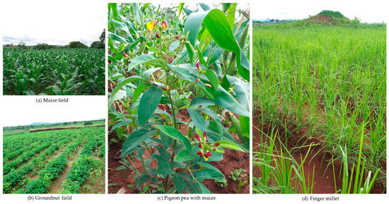
Figure 2.
Examples of crops photographed in the study locations during the 2019/2020 growing season.
2.3. Data Processing
2.3.1. Radar Data Processing
The Sentinel-1 IW images were preprocessed in twelve steps (Figure 3) using the SNAP toolbox. The data were first split into sub-swaths to focus on the two study locations and reduce the size of the image to improve processing efficiency. Due to the reduced sensitivity to displacement gradient when the Sentinel-1 satellite is scanning, split-bandwidth interferometry also allows for more multilooking than is possible with standard interferometric phase in highly deformed areas such as the hilly landscape in northern Malawi. Splitting the images further improves accuracy in low coherence areas [36]. The orbit state vectors provided in the metadata of an SAR product are generally not accurate and can be refined with the precise orbit files. These files are available days-to-weeks after the generation of the product [47]. The orbit file operator in the SNAP toolbox automatically downloads the latest released orbit file and applies it to the image so that the image can be geocoded more precisely.
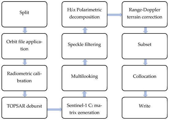
Figure 3.
Major preprocessing steps for the Sentinel-1 synthetic aperture radar images.
The next preprocessing step was to calibrate the images. SAR calibration produces imagery with pixel values that correlate with the radar backscatter of the captured scene [48]. Applying the radiometric correction operator also produces images that can be compared with other SAR images acquired with different sensors or acquired from the same sensor but at different times, in different orbits, or processed by different processors. Calibrating the images used in this study is thus relevant, since a multitemporal analysis is to be performed [47]. Creating the multitemporal multiband image requires stacking several Sentinel-1 data collected over the growing season and fusing them with optical data. The calibration process was followed by debursting. Sentinel-1 IW SLC products consist of one image per swath per polarization. The IW products that were used have three swaths. Each sub-swath image consists of a series of bursts. Each burst was processed as a unique SLC image. To merge all these bursts into a single SLC image, the TOPSAR Deburst and Merge operator in the SNAP toolbox was applied. The polarimetric matrix generation process was used to generate a covariance matrix from the Sentinel-1 C-band SAR data [49]. Dual polarimetric SAR sensors collect half of the total polarimetric information involved in fully polarimetric imagery or quad polarization [50]. This implies that the resolution cell at each time point is defined by a 2 × 2 covariance (C2) matrix that is obtained from C3 (representing the average polarimetric information extracted from a set of neighboring pixels). The resulting C2 matrix is represented by Equation (1).
Dual polarization imagery has only diagonal elements. As such, the matrix with off-diagonal components were set to zero and do not follow a complex Wishart distribution; but, the two diagonal blocks (1 by 1) follow a complex Wishart distribution [51,52].
Multilooking and polarimetric speckle filtering were applied to reduce speckle noise. The presence of speckle intensity fluctuations in SLC SAR imagery is the result of the nature of coherent image formation during SAR data collection [47]. Each radar resolution cell contains multiple scatters, each of which contributes to the overall signal returned from the resolution cell. The phase obtained from each scatter is effectively random because the radar wavelength is normally much smaller than the size of the resolution cell. The signals from each scatter may be summed according to the principle of superposition, resulting in constructive and destructive interference [53]. Low reflectivity occurs in cells where destructive interference dominates, while constructive interference dominates in cells where high reflectivity prevails. Consequently, the phenomenon of speckle occurs on the image. Multilooking, which is achieved by dividing the signal spectrum and then incoherently averaging the recovered sub-images of an SAR image, is widely used to reduce these speckles in conventional SAR signal processing [54]. The Boxcar polarimetric speckle filtering method with a 5 × 5 window size was used to further reduce speckle noise in the image while preserving the complex information of all the bands, enhancing interpretation, and improving their ability for quantitative analysis. The Boxcar filter is the simplest filter that locates similar pixels by a moving window with the predefined size. The filter reduces the speckle phenomenon while producing a blurring visual effect [55].
Polarimetric decomposition was used to separate different scattering contributions and provide information about the scattering process [56]. Polarimetric decompositions are techniques used to generate polarimetric discriminators that can be used for analysis, interpretation, and classification of SAR data [57]. The H/α dual-polarized decomposition of VV–VH dual-polarization with the window size of 5 × 5 was performed. H/α polarimetric decomposition is an entropy-based method based on the theory that the polarization scattering characteristics can be represented by the space of the entropy and the averaged scattering angle α employing the eigenvalue analysis of Hermitian matrices [52]. The H/α polarimetric decomposition method proposed by Cloude and Pottier [52] is widely used for land cover classification and object recognition. The method has good properties such as rotation invariance, irrelevance to specific probability density distributions, and covers the whole scattering mechanism space [58]. Only the 2 × 2 covariance matrix was derived, because the Sentinel-1 product is dual-polarized. The entropy and alpha images were derived from the H/α dual-polarized decomposition and used for the present analysis.
During range-Doppler terrain correction [59], a Shuttle Radar Topography Mission (SRTM) digital elevation model (DEM) was downloaded automatically from the SNAP toolbox to fulfill orthorectification [60]. Terrain-correcting the images is important because the discrepancies in topographical variations of a scene and the tilt of the satellite sensor distort distances in SAR images. Applying terrain correction compensates for these distortions and make features appear as close as possible to real-world features [59]. The final image was resampled into 3-m to conform with the optical PlanetScope data. A subset of all the images is clipped and a stack was then made of all the layers.
2.3.2. Optical Data Processing
For the Sentinel-2 and PlanetScope data, we applied atmospheric correction, topographic correction, resampling, band stacking, seamless mosaicking, and image sub-setting as preprocessing steps. The Sentinel-2 Level-2A bottom-of-atmosphere (BOA) products we acquired are already atmospherically corrected. Examples of preprocessed natural color and grayscale images of the radar and optical data of the study locations are shown in Figure 4.
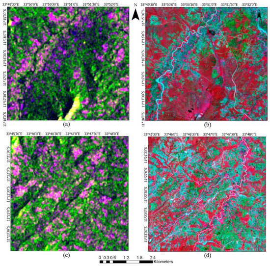
Figure 4.
False color images of the Thimalala and Edundu, represented by (a,c) Sentinel-1 C11 and C22 backscatter response (RGB = C11, C22, C11/C22) on 18/01/2020; (b,d) preprocessed Sentinel-2 image (RGB = NIR, red, green) on 07/01/2020.
2.4. Image Fusion
Images from different spectral bands have the same geometric information [61]. Based on this principle of satellite images, Gašparović et al. [62] developed an image fusion method known as the P + XS fusion, in which an image is perceived as a function whose sampling corresponds to the discrete matrix form of the image [63]. The P + XS method introduces the geometry information of a higher resolution image by aligning all edges of the higher resolution image with each lower resolution multispectral band. To obtain the spectral information for the fused image, the method assumes that images captured in different spectral bands share common geometric information and that the higher resolution image can be approximated as a linear combination of the high-resolution multispectral bands [64,65]. Guided by this principle, each Sentinel-2 band was fused with the corresponding high spatial resolution PlanetScope band that shares similar spectral characteristics. He et al. [65] observed that using the P + XS method can better preserve sharp discontinuities such as edges and object contours on an image. The objective of the fusion was to produce higher resolution Sentinel-2 multispectral fused images from the original low-resolution Sentinel-2 and high-resolution PlanetScope images.
The smoothing filter-based intensity modulation (SFIM) [66] was used to fuse the Sentinel-2 and PlanetScope images. The SFIM aims to produce fused images that have the highest spatial resolution in the same multispectral bands of the original low-resolution images. The lower spatial resolution Sentinel-2 bands were fused with the higher spatial resolution PlanetScope bands based on the principles of the P + XS method. The corresponding bands of the PlanetScope were alternatively used as the high spatial resolution band in place of panchromatic bands (Table 3). The SFIM technique improves spatial details while keeping the spectral properties of the images. The digital number (DN) value of the fused band is defined as:
where is the DN value of the fused band i, is the corresponding lower spatial-resolution band I, resampled to the same high resolution as Y, Y represents the high spatial resolution panchromatic band, and represents the Y band being averaged by the low-pass filtering.
Table 3.
Fusion pairs of Sentinel-2 and PlanetScope bands.
For Thimalala, the Sentinel-2 images acquired on 07/01/2020 were fused with the PlanetScope images on 23/02/2020. For Edundu, the Sentinel-2 images acquired on 07/01/2020 and 23/02/2020 were fused with the PlanetScope images taken on 01/04/2020 separately. Figure 5 shows examples of subset image cropped from the originally preprocessed Sentinel-2 images and the fused (Sentinel-2 + PlanetScope) image. It can be observed from the images that the fused data are clearer than the original (Figure 5).
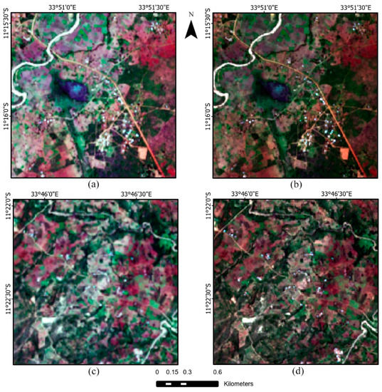
Figure 5.
True color composites of the subset images from (a) Sentinel-2 image for Thimalala on 07/01/2020; (b) fused images for Thimalala; (c) Sentinel-2 images for Edundu on 07/01/2020; (d) fused images for Edundu.
2.5. Image Classification
Fourteen (14) crop types in total and eight (8) land cover classes identified in the two study locations were used as the schema of the classification. The crop type classes were identified through field data collection. The land cover types were identified based on field observations during ground truth data collection, as well as from very high resolution Google Earth Pro and DigitalGlobe images. The supervised random forest (RF) machine learning algorithm [67] in ENVI 5.3 was used for the classification. As a non-parametric method, RF benefits from including categorical and continuous datasets based on well-developed rules and does not require training data to come from a unimodal distribution [68]. An RF is generated through the creation of a series of decorrelated decision trees using bootstrapping, thus solving the problem of overfitting and producing accurate results [67]. Tuning parameters, such as the number of trees and the number of split candidate predictors, are generally chosen based on the out-of-bag (OOB) prediction error. RF uses the OOB samples for cross-validation, and once the OOB errors stabilize at a reasonably large number of trees, training can be concluded. In this study, the model we used in each experiment consisted of 500 trees and the number of features to split the nodes was set to half of the features within the corresponding input dataset. Accuracy of RF classification is often very high, even when based on many input features such as multitemporal images [69].
2.6. Post-Classification Processing
A 3 × 3 filter with the majority vote was applied to remove the salt-and-pepper effect in the classified images. Accuracy assessment was performed to evaluate the performance of each classification experiment using the ground truth data acquired from fieldwork, Google Earth Pro, and DigitalGlobe images based on Congalton [70]. The overall accuracy (OA), producer’s accuracy (PA), user’s accuracy (UA), and the Kappa coefficients were computed for each of the five experiments to determine the best-performing model for identifying crop types and land cover categories. The OA describes the proportion of pixels correctly classified, with 85% or more generally accepted as the threshold for a good classification. The PA is the map accuracy from the point of view of the map producer. It explains how often features on the ground are correctly shown on the classified map, or the probability that a certain land cover type on the ground is classified as such [71]. The UA, on the other hand, is the accuracy from the point of view of a map user. It describes how often the features identified on the map will be present on the ground [71]. The Kappa coefficient is the ratio of the agreement between the classifier output and reference data, and the probability that there is no chance agreement between the classified and the reference data [70].
3. Results
Table 4 presents the results of the accuracy assessment for all five experiments. For the Sentinel-1-only experiment, the overall accuracies of both locations were lower than 50%. For the Sentinel-2-only experiment, the accuracies increased significantly to 72% and 74%, respectively, but were still lower than expected for an ideal classification. The water class was better extracted in the Sentinel-2-only experiment, compared with the Sentinel-1-only experiment. When using the fused image of Sentinel-2 and PlanetScope, the introduction of the relatively higher spatial resolution image of 3 m added more detail to the classes, though it failed to accurately identify groundnut crops. The overall accuracy increased to 76.03% for Thimalala and 84.12% for the Edundu location.
Table 4.
Comparison of the accuracy assessment results of the random forest classification.
In the fourth experiment, we made a stack of the fused Sentinel-2 and PlanetScope images and the Sentinel-1 C2 matrix (Sentinel-2 and PlanetScope fused image + Sentinel-1 C2 matrix). The addition of the Sentinel-1 C2 matrix generated minor improvements on the Sentinel-2 + PlanetScope experiment in experiment (iii), as observed in the improved accuracy statistics (Table 4). The combination of optical and SAR data resulted in a slightly better increment (5%) in the overall accuracy for the Thimalala site, compared to the Edundu site (0.42%), but the accuracies were still lower than the accepted value for a good classification.
In the final experiment, a multiband image was created comprising the fused image from the fourth experiment and the H/α polarimetric decomposition (i.e., the fusion of Sentinel-2 + PlanetScope + Sentinel-1 C2 matrix + H/α polarimetric decomposition). This final experiment produced results that outperformed all the other integration of images. The overall accuracies from this final experiment exceeded 85% in both locations, which is the threshold for a good classification. Overall, the accuracies improved by 13.53% and 11.7% for Thimalala and Edundu, respectively, compared with the Sentinel-2-only classification.
Table 5 shows the PA and UA accuracies for the experiment (v). Crops such as bambara nuts (100%), groundnuts (90%), maize (100%), tobacco (87.5%), and tomato (100%) had high PAs with equally high UAs, meaning the method accurately identified the crops. The corresponding UAs also showed that the maps are useful for identifying these common crops on the landscape from the user’s perspective. Crops including banana, onion, and sweet potato were very few in the landscape and only a few samples were obtained. As such, our model could not adequately assess these classes. This explains the nature of the PAs and UAs for these crop classes (Table 5). Land cover classes such as forest, shrubland, untarred road, and water also had high PAs, compared to settlement, bare rock, and tarred roads, which had low PAs. Corresponding UAs were within a similar range to the PAs.
Table 5.
Summary of classification accuracies of Thimalala using the fused image of Sentinel-2 and PlanetScope, Sentinel-1 C2 matrix, and H/α polarimetric decomposition.
Figure 6 and Figure 7 show the maps generated for the various experiments for the two locations. Figure 6a and Figure 7a show results for the Sentinel-1-only experiment for Thimalala and Edundu, respectively, while Figure 6b and Figure 7b show the results for the Sentinel-2-only experiment for the two village areas. The results reflect the poor accuracies generated from the experiments (see Table 4 and Table 5). Results presented in Figure 6c and Figure 7c show that the various classes are more identifiable than in the foregoing experiments in both locations, while Figure 6d and Figure 7d reflect the minor improvement of accuracies when moving from the experiment (iii) to (iv) (see Table 4). It can be seen in Figure 6e and Figure 7e that the classification improved with the introduction of the H/α decomposition layer. In terms of the distribution and dominance of crop types, both Figure 6 and Figure 7 show that maize is the dominant crop type in both study locations. Tobacco crops are also common in both areas and are observed to have, on average, larger sizes than most food croplands. Intercropped farmlands, which are mainly maize intercropped with other legumes and pumpkins, are also prominent on the landscape in both locations. Though the classification was able to identify intercropped fields, most likely maize with other crops that are equally tall, such as pigeon pea or cassava, it was, however, not able to identify which specific crop combinations (e.g., maize/bean and maize/soybean) constitute each intercropped farm. Croplands that were not classified into any of the individual categories were grouped into the mixed/intercropped class. As expected, croplands are mostly in low-lying valley areas. Shrublands and forests are the most dominant land cover types on hills and hillslopes in both locations. The forests are mostly surrounded by shrublands interspersed with some farmlands, especially in the Thimalala area.
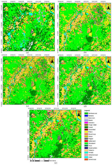
Figure 6.
Classification results of Thimalala area (a) using Sentinel-1 only; (b) using Sentinel-2 only; (c) using the fused image of Sentinel-2 and PlanetScope; (d) using the fused image and Sentinel-1 C2 matrix; (e) using the fused image, Sentinel-1 C2 matrix, and H/α polarimetric decomposition.
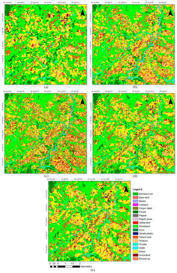
Figure 7.
Classification results of Edundu area (a) using Sentinel-1 only; (b) using Sentinel-2 only; (c) using the fused image of Sentinel-2 and PlanetScope; (d) using the fused image and Sentinel-1 C2 matrix; (e) using the fused image, Sentinel-1 C2 matrix, and H/α polarimetric decomposition.
Overall, the results show that the fused images outperformed the single images in identifying crop types and land cover categories in both study locations. The OAs improved as the number of image combinations increased. The image fused with the Sentinel-1 H/α polarimetric decomposition outperformed all the other fused image experiments. The optical data (Sentinel-2 only) outperformed the radar data (Sentinel-1-only) in identifying crop types and land cover in both study locations by a wide margin.
4. Discussion
The study reveals useful observations about crop type and land cover identification in heterogenous smallholder agricultural landscapes. The experiments provide evidence that to effectively identify crop types, cropping systems, and land cover using pixel-based classification, a combination of multitemporal satellite data from different sensors can be used. We show that the fusion of Sentinel-2 and PlanetScope optical images integrated with Sentinel-1 C2 matrix and Sentinel-1 H/α polarimetric decomposition was the most effective in generating high-accuracy crop type and land cover maps (Table 4). The degree of accuracy increased from the experiment (i) as the number of images integrated for the classification increased. Using only the Sentinel-1 images produced OAs lower than 50% for both locations, similar to observations made by Mercier et al. [72]. When the Sentinel-1 C2 matrix was fused with Sentinel-2, the accuracies improved for both study locations. Fusing the two optical images further improved the classification results of the Sentinel-2-only by 3.95% and 10.04% for Thimalala and Edundu, respectively. Orynbaikyzy et al. [73] noted similarly that fusing Sentinel-1 and Sentinel-2 data improved the results of crop classification in Northern Germany, as did Mercier et al. [72] in Paragominas (Brazil). Gašparović et al. [62] observed a similar improvement when they integrated Sentinel-2 with PlanetScope for vegetation mapping and monitoring. There were only a few banana, onion, and sweet potato samples in the validation data because these crops are generally scarce in the agricultural landscape of both study locations. They are also often planted on relatively smaller plot sizes. A such, the PAs and UAs for these crop classes show that the assessment might have been less inaccurate (Table 5). The foregoing explanation is one of the main limitations of classifying crop types in complex heterogeneous smallholder agriculture landscapes, as highlighted in other studies [8]. At the same time, the observation presents an opportunity for future studies to explore other approaches to capturing such rare crops using image classification.
The observation that fusing Sentinel-1 and the optical data improved crop type mapping is also consistent with findings of other studies that have combined radar and optical data for crop and land cover type mapping [22,65]. The finding provides further evidence of the contribution of dual-polarized Sentinel-1 data for accurate crop and land cover classification. We conclude that the 13.53% (Thimalala) and 11.7% (Edundu) improvements in overall accuracy on the Sentinel-2-only classification is because of the integration of the multitemporal datasets from all the various sensors with the Sentinel-1 H/α polarimetric decomposition. This finding suggests that adding more multitemporal images could further improve the OAs, PAs, and UAs, and using only a unitemporal image produces underwhelming results. Previous studies have also found that integrating the H/α polarimetric decomposition information with other data achieves better accuracy in complex agricultural landscapes than other classical methods [74,75,76]. Dual-polarized data such as Sentinel-1 are a valuable data resource for decomposing radar data to map crop types [73]. The poor accuracy from the Sentinel-1-only experiment (i) is, therefore, likely the result of the design of our experiment (i). The two bands of the Sentinel-1 IW mode compared to the several bands available from Sentinel-2 and PlanetScope and the use of the random forest algorithm may explain the poor accuracy from the Sentinel-1-only classification [77]. Quad-polarized data are known to perform better in identifying crop types when integrated with other data [78]. Future crop type mapping in the study locations should, therefore, integrate time series quad-polarized H/α polarimetric decomposition, if available, with available time series optical data to achieve better accuracies.
The combination of multitemporal, multispectral, and multisensor data to map crops in such heterogeneous landscapes suggests that in areas of high cloud cover where optical data collection is not feasible, combining data with different spectral characteristics, including radar and optical data, holds the potential for reliable mapping of crop types and land cover for building crop type inventories. The classification outcomes indicate that the multitemporal routine of fusing the quality high-resolution optical images (PlanetScope) with radar data and the random forest classification approach outperformed the Sentinel-1-only data. Malawi, similar to many other locations in the tropics, has dense cloud cover during critical stages of crop growth but has limited coverage of high temporal resolution remote sensing satellites. This makes it difficult to acquire time series optical data for monitoring crop growth and mapping crop diversity. Clouds are often cited as the main advantage of using radar for mapping land cover. Being able to routinely map the landscapes in such resource-poor contexts using a combination of images from different sensors is critical to creating crop inventory maps by local officials to facilitate food security and environmental management decision-making [79]. The timing and quality of satellite observations play a crucial role in the accuracy of classification to identify crops [77]. Even though the seasonal satellite data we used contributed to the overall accuracy, only a few of the cloud-free optical images were obtained for the start of the growing season due to heavy cloud cover. As such, it was difficult for our optimal model to effectively separate the different crop combinations on intercropped farms, even though some intercropped fields were identified. The experiment (v) was able to identify the distribution of crops, with maize being the most common crop, a finding consistent with the maizification of Malawi narrative found in other studies, a phenomenon attributed to government agricultural policies [79]. Future studies can overcome the challenge of inaccurate identification of intercropped fields by using images acquired at the start of the growing season when the specific crop combinations on intercropped fields are visible to satellite sensors and can be captured and separated by image classification algorithms.
A combination of field ground truth data and samples from Google Earth Pro and DigitalGlobe images, as well as ancillary information, was used to train and validate the random forest algorithm to attain more than 85% accuracy in the experiment (v) (Table 4). The accuracy attained suggests that using reference data from diverse sources can improve classification results, as observed in other studies [23,74]. This observation implies that the level of accuracy obtained in our experiments can be further improved with more training and validation samples. In future, crowdsourcing should be used to collect more field samples by training farmers to use smartphones and other spatial data collection applications and tools to geolocate and record farm and ancillary information for training and validating classifiers. Using crowdsourcing to collect crop type samples has been experimented with in other contexts and found to have contributed to getting large volumes of training data for mapping crop types more accurately [23]. Adding more training samples will also allow classification algorithms to identify the specific crops in intercropped fields.
5. Conclusions
The outcomes of the experiments conducted in this study highlight the importance of exploiting the capabilities of various satellite sensors to create high temporal resolution images for mapping crop types and land cover in smallholder agriculture areas where the landscapes tend to be more heterogeneous. Both individual Sentinel-1 and Sentinel-2 images failed to produce high-accuracy crop type and land cover maps. The overall accuracy and Kappa coefficients of the classification improved as the number of images increased and the spatial resolution improved. The fusion of Sentinel-1 C2 matrix, Sentinel-2, and PlanetScope optical data with the Sentinel-1 H/α polarimetric decomposition outperformed all other combinations of images. Fusing the images created high temporal resolution data, with Sentinel-1 contributing the greatest number of images due to the ability of SAR to penetrate cloud cover. Though processing time may increase due to the high volume of data being integrated, the fact that acceptable accuracies were achieved is crucial. In the tropical areas of SSA where cloud cover is often dense during the growing season, this study demonstrates that computing the H/α polarimetric decomposition from cloud-penetrating radar data and fusing it with other high- and moderate-resolution optical data can be very cost-effective for developing large-scale crop inventory data. Several studies have shown how these current and emerging sensors can be harmonized to map crop types and land cover for use as decision support tools to facilitate food security decision-making. Our study makes a valuable contribution to the literature on image fusion for crop type mapping. Intercropping is predominant in most smallholder contexts in SSA, but our experiments could not adequately identify the individual crops on such intercropped fields due to data constraints. Since the H/α polarimetric decomposition image contributed to the improved accuracy of the experiments, future studies should apply H/α polarimetric decomposition from quad-polarized data, if available, with early-season optical data and more ground truth samples to better identify the mix of crops on intercropped farms. Given the current fast pace of sensor and image processing algorithm development, it is possible to apply the method explored in this study on an operational basis to develop crop inventory data at larger scales to guide decision-making for improved food security and environmental management in cloud-dense, resource-poor locations. The approach used in this study can be used by local agriculture decision-makers to map and monitor cropping patterns and land cover change dynamics over time to build land cover inventory datasets.
Author Contributions
Conceptualization, I.L., J.W., and D.K.; methodology, X.S., J.W. and D.K.; software, X.S.; validation, J.W., X.S., and D.K.; formal analysis, X.S.; investigation, D.K.; resources, I.L., J.W.; data curation, D.K. and X.S.; writing—original draft preparation, D.K. and X.S.; writing—review and editing, D.K., X.S., J.W., I.L. and R.B.K.; visualization, X.S.; supervision, I.L., J.W.; project administration, R.B.K., E.L. and L.D.; funding acquisition, I.L., R.B.K. and J.W. All authors have read and agreed to the published version of the manuscript.
Funding
This research was funded through the 2017–2018 Belmont Forum and BiodivERsA joint call for research proposals, under the BiodivScen ERA-Net COFUND program, and funded by the Natural Sciences and Engineering Research Council of Canada (NSERC Grant# 523660-2018). Additionally, XS was funded through the Natural Sciences and Engineering Research Council of Canada (NSERC) Discovery Grant awarded to Dr. Jinfei Wang.
Institutional Review Board Statement
Ethical approval for the research was granted by the Western University Non-Medical Research Ethics Board (NMREB# 113568).
Data Availability Statement
Sentinel-1 and Sentinel-2 data are publicly available from the European Space Agency’s website https://scihub.copernicus.eu/dhus/#/home (accessed on 28 December 2020). Restrictions apply to the availability of PlanetScope data. Data were obtained from Planet Labs Inc. as part of their Education and Research Program. The data are available for purchase from https://www.planet.com/login/?mode=signup (accessed on 28 December 2020) with the permission of Planet Labs Inc.
Acknowledgments
We are grateful to all the farmers who allowed us to work on their farms during this research project. We are also thankful to the village headmen for allowing the research team to work in their communities. The authors thank Gladson Simwaka, the research assistant, for the hard work in collecting the data. We are also immeasurably grateful to the staff of Soils, Food and Healthy Communities, our Malawi partner. We are grateful to the International Development Research Centre (IDRC) for the Doctoral Awards (IDRA 2018, 108838-013) and the Micha and Nancy Pazner Fieldwork Award for supporting the fieldwork financially. Finally, we are thankful to Planet Labs Inc. for making the PlanetScope data freely available to support the doctoral research of the lead author.
Conflicts of Interest
The authors declare no conflict of interest.
References
- Moreau, D.; Pointurier, O.; Nicolardot, B.; Villerd, J.; Colbach, N. In which cropping systems can residual weeds reduce nitrate leaching and soil erosion? Eur. J. Agron. 2020, 119, 126015. [Google Scholar] [CrossRef]
- Muoni, T.; Koomson, E.; Öborn, I.; Marohn, C.; Watson, C.A.; Bergkvist, G.; Barnes, A.; Cadisch, G.; Duncan, A. Reducing soil erosion in smallholder farming systems in east Africa through the introduction of different crop types. Exp. Agric. 2020, 56, 183–195. [Google Scholar] [CrossRef]
- Saleem, M.; Pervaiz, Z.H.; Contreras, J.; Lindenberger, J.H.; Hupp, B.M.; Chen, D.; Zhang, Q.; Wang, C.; Iqbal, J.; Twigg, P. Cover crop diversity improves multiple soil properties via altering root architectural traits. Rhizosphere 2020, 16, 100248. [Google Scholar] [CrossRef]
- Ouyang, F.; Su, W.; Zhang, Y.; Liu, X.; Su, J.; Zhang, Q.; Men, X.; Ju, Q.; Ge, F. Ecological control service of the predatory natural enemy and its maintaining mechanism in rotation-intercropping ecosystem via wheat-maize-cotton. Agric. Ecosyst. Environ. 2020, 301, 107024. [Google Scholar] [CrossRef]
- Pakeman, R.J.; Brooker, R.W.; Karley, A.J.; Newton, A.C.; Mitchell, C.; Hewison, R.L.; Pollenus, J.; Guy, D.C.; Schöb, C. Increased crop diversity reduces the functional space available for weeds. Weed Res. 2020, 60, 121–131. [Google Scholar] [CrossRef]
- Richards, A.; Estaki, M.; Úrbez-Torres, J.R.; Bowen, P.; Lowery, T.; Hart, M. Cover Crop Diversity as a Tool to Mitigate Vine Decline and Reduce Pathogens in Vineyard Soils. Diversity 2020, 12, 128. [Google Scholar] [CrossRef]
- FAO. Save and Grow. A Policymaker’s Guide to the Sustainable Intensification of Smallholder Crop Production; FAO: Rome, Italy, 2011. [Google Scholar]
- Lowder, S.K.; Skoet, J.; Raney, T. The number, size, and distribution of farms, smallholder farms, and family farms worldwide. World Dev. 2016, 87, 16–29. [Google Scholar] [CrossRef]
- Rapsomanikis, G. The Economic Lives of Smallholder Farmers: An Analysis Based on Household Data from Nine Countries; I5251E/1/12.15; Food and Agriculture Organization of the United Nations (FAO): Rome, Italy, 2015. [Google Scholar]
- Ricciardi, V.; Ramankutty, N.; Mehrabi, Z.; Jarvis, L.; Chookolingo, B. How much of the world’s food do smallholders produce? Glob. Food Secur. 2018, 17, 64–72. [Google Scholar] [CrossRef]
- Samberg, L.H.; Gerber, J.S.; Ramankutty, N.; Herrero, M.; West, P.C. Subnational distribution of average farm size and smallholder contributions to global food production. Environ. Res. Lett. 2016, 11, 124010. [Google Scholar] [CrossRef]
- Kpienbaareh, D.; Bezner Kerr, R.; Luginaah, I.; Wang, J.; Lupafya, E.; Dakishoni, L.; Shumba, L. Spatial and ecological farmer knowledge and decision-making about ecosystem services and biodiversity. Land 2020, 9, 356. [Google Scholar] [CrossRef]
- Burke, M.; Lobell, D.B. Satellite-based assessment of yield variation and its determinants in smallholder African systems. Proc. Natl. Acad. Sci. USA 2017, 114, 2189–2194. [Google Scholar] [CrossRef] [PubMed]
- Plourde, J.D.; Pijanowski, B.C.; Pekin, B.K. Evidence for increased monoculture cropping in the Central United States. Agric. Ecosyst. Environ. 2013, 165, 50–59. [Google Scholar] [CrossRef]
- Espey, J. Data for Development: A Needs Assessment for SDG Monitoring and Statistical Capacity Development; Sustainable Development Solutions Network: New York, NY, USA, 2015. [Google Scholar]
- Christiaensen, L.; Demery, L. Agriculture in Africa: Telling Myths from Facts; The World Bank: Washington, DC, USA, 2017; ISBN 1464811342. [Google Scholar]
- Snapp, S.; Bezner Kerr, R.; Ota, V.; Kane, D.; Shumba, L.; Dakishoni, L. Unpacking a crop diversity hotspot: Farmer practice and preferences in Northern Malawi. Int. J. Agric. Sustain. 2019, 17, 172–188. [Google Scholar] [CrossRef]
- Atzberger, C. Advances in remote sensing of agriculture: Context description, existing operational monitoring systems and major information needs. Remote Sens. 2013, 5, 949–981. [Google Scholar] [CrossRef]
- Thenkabail, P.S. Hyperspectral data analysis of the world’s leading agricultural crops (Conference Presentation). In Proceedings of the Micro-and Nanotechnology Sensors, Systems, and Applications X, International Society for Optics and Photonics, Orlando, FL, USA, 14 May 2018; Volume 10639, p. 1063914. [Google Scholar]
- Fisette, T.; Rollin, P.; Aly, Z.; Campbell, L.; Daneshfar, B.; Filyer, P.; Smith, A.; Davidson, A.; Shang, J.; Jarvis, I. AAFC annual crop inventory. In Proceedings of the 2013 Second International Conference on Agro-Geoinformatics (Agro-Geoinformatics), Fairfax, VA, USA, 12–16 August 2013; pp. 270–274. [Google Scholar]
- Inglada, J.; Arias, M.; Tardy, B.; Hagolle, O.; Valero, S.; Morin, D.; Dedieu, G.; Sepulcre, G.; Bontemps, S.; Defourny, P.; et al. Assessment of an operational system for crop type map production using high temporal and spatial resolution satellite optical imagery. Remote Sens. 2015, 7, 12356–12379. [Google Scholar] [CrossRef]
- Kpienbaareh, D.; Luginaah, I. Mapping burnt areas in the semi-arid savannahs: An exploration of SVM classification and field surveys. GeoJournal 2019, 1–14. [Google Scholar] [CrossRef]
- Wang, S.; Di Tommaso, S.; Faulkner, J.; Friedel, T.; Kennepohl, A.; Strey, R.; Lobell, D.B. Mapping crop types in southeast India with smartphone crowdsourcing and deep learning. Remote Sens. 2020, 12, 2957. [Google Scholar] [CrossRef]
- Khalil, C.A.; Conforti, P.; Ergin, I.; Gennari, P. Defining small scale food producers to monitor target 2.3 of the 2030 Agenda for Sustainable Development. Working Paper ESS 17-12. Ecol. Soc. 2012, 17, 44. [Google Scholar] [CrossRef]
- Wang, S.; Azzari, G.; Lobell, D.B. Crop type mapping without field-level labels: Random forest transfer and unsupervised clustering techniques. Remote Sens. Environ. 2019, 222, 303–317. [Google Scholar] [CrossRef]
- Kaplan, G.; Avdan, U. Sentinel-1 and Sentinel-2 data fusion for wetlands mapping: Balikdami, Turkey. Int. Arch. Photogramm. Remote Sens. Spat. Inf. Sci. 2018, XLII-3, 729–734. [Google Scholar] [CrossRef]
- Slagter, B.; Tsendbazar, N.-E.; Vollrath, A.; Reiche, J. Mapping wetland characteristics using temporally dense Sentinel-1 and Sentinel-2 data: A case study in the St. Lucia wetlands, South Africa. Int. J. Appl. Earth Obs. Geoinf. 2020, 86, 102009. [Google Scholar] [CrossRef]
- Kannaujiya, S.; Chattoraj, S.L.; Jayalath, D.; Bajaj, K.; Podali, S.; Bisht, M.P.S. Integration of satellite remote sensing and geophysical techniques (electrical resistivity tomography and ground penetrating radar) for landslide characterization at Kunjethi (Kalimath), Garhwal Himalaya, India. Nat. Hazards 2019, 97, 1191–1208. [Google Scholar] [CrossRef]
- Yan, S.; Shi, K.; Li, Y.; Liu, J.; Zhao, H. Integration of satellite remote sensing data in underground coal fire detection: A case study of the Fukang region, Xinjiang, China. Front. Earth Sci. 2019, 14, 1–12. [Google Scholar] [CrossRef]
- Venter, Z.S.; Brousse, O.; Esau, I.; Meier, F. Hyperlocal mapping of urban air temperature using remote sensing and crowdsourced weather data. Remote Sens. Environ. 2020, 242, 111791. [Google Scholar] [CrossRef]
- Frampton, W.J.; Dash, J.; Watmough, G.; Milton, E.J. Evaluating the capabilities of Sentinel-2 for quantitative estimation of biophysical variables in vegetation. ISPRS J. Photogramm. Remote Sens. 2013, 82, 83–92. [Google Scholar] [CrossRef]
- Gama, A.C.; Mapemba, L.D.; Masikat, P.; Tui, S.H.-K.; Crespo, O.; Bandason, E. Modeling Potential Impacts of Future Climate Change in Mzimba District, Malawi, 2040–2070: An Integrated Biophysical and Economic Modeling Approach; Intl Food Policy Res Inst: New Delhi, India, 2014; Volume 8. [Google Scholar]
- Li, G.; Messina, J.P.; Peter, B.G.; Snapp, S.S. Mapping land suitability for agriculture in Malawi. Land Degrad. Dev. 2017, 28, 2001–2016. [Google Scholar] [CrossRef]
- Chinsinga, B. The Political Economy of Agricultural Policy Processes in Malawi: A Case Study of the Fertilizer Subsidy Programme; Working Paper 39; Future Agricultures Consortium: Brighton, UK, 2012. [Google Scholar]
- Jiang, H.; Feng, G.; Wang, T.; Bürgmann, R. Toward full exploitation of coherent and incoherent information in Sentinel-1 TOPS data for retrieving surface displacement: Application to the 2016 Kumamoto (Japan) earthquake. Geophys. Res. Lett. 2017, 44, 1758–1767. [Google Scholar] [CrossRef]
- Abdikan, S.; Sanli, F.B.; Ustuner, M.; Calò, F. Land cover mapping using sentinel-1 SAR data. Int. Arch. Photogramm. Remote Sens. Spat. Inf. Sci. 2016, 41, 757. [Google Scholar] [CrossRef]
- Ban, Y. Synergy of multitemporal ERS-1 SAR and Landsat TM data for classification of agricultural crops. Can. J. Remote Sens. 2003, 29, 518–526. [Google Scholar] [CrossRef]
- Stefanski, J.; Kuemmerle, T.; Chaskovskyy, O.; Griffiths, P.; Havryluk, V.; Knorn, J.; Korol, N.; Sieber, A.; Waske, B. Mapping land management regimes in western Ukraine using optical and SAR data. Remote Sens. 2014, 6, 5279–5305. [Google Scholar] [CrossRef]
- ESA. Sentinel-2 Mission Requirements Document, Issue 2. 2010. Available online: http://esamultimedia.esa.int/docs/GMES/Sentinel-2_MRD.pdf (accessed on 25 January 2018).
- Jin, Z.; Azzari, G.; You, C.; Di Tommaso, S.; Aston, S.; Burke, M.; Lobell, D.B. Smallholder maize area and yield mapping at national scales with Google Earth Engine. Remote Sens. Environ. 2019, 228, 115–128. [Google Scholar] [CrossRef]
- P.L. Inc. Planet Imagery and Archive. 2020. Available online: https://www.planet.com/products/planet-imagery/ (accessed on 15 August 2020).
- Kotchenova, S.Y.; Vermote, E.F. Validation of a vector version of the 6S radiative transfer code for atmospheric correction of satellite data. Part II. Homogeneous Lambertian and anisotropic surfaces. Appl. Opt. 2007, 46, 4455–4464. [Google Scholar] [CrossRef]
- Francini, S.; McRoberts, R.E.; Giannetti, F.; Mencucci, M.; Marchetti, M.; Scarascia Mugnozza, G.; Chirici, G. Near-real time forest change detection using PlanetScope imagery. Eur. J. Remote Sens. 2020, 53, 233–244. [Google Scholar] [CrossRef]
- Kokhan, S.; Vostokov, A. Application of nanosatellites PlanetScope data to monitor crop growth. In Proceedings of the E3S Web of Conferences, Lublin, Poland, 17–20 September 2020; Volume 171, p. 2014. [Google Scholar]
- Shi, Y.; Huang, W.; Ye, H.; Ruan, C.; Xing, N.; Geng, Y.; Dong, Y.; Peng, D. Partial least square discriminant analysis based on normalized two-stage vegetation indices for mapping damage from rice diseases using PlanetScope datasets. Sensors 2018, 18, 1901. [Google Scholar] [CrossRef] [PubMed]
- ESA. ESA Sentinel Application Platform v6.0.0; ESA: Paris, France, 2018. [Google Scholar]
- Schwerdt, M.; Schmidt, K.; Ramon, N.T.; Klenk, P.; Yague-Martinez, N.; Prats-Iraola, P.; Zink, M.; Geudtner, D. Independent system calibration of Sentinel-1B. Remote Sens. 2017, 9, 511. [Google Scholar] [CrossRef]
- McNairn, H.; Brisco, B. The application of C-band polarimetric SAR for agriculture: A review. Can. J. Remote Sens. 2004, 30, 525–542. [Google Scholar] [CrossRef]
- Ainsworth, T.L.; Kelly, J.; Lee, J.-S. Polarimetric analysis of dual polarimetric SAR imagery. In Proceedings of the 7th European Conference on Synthetic Aperture Radar, Friedrichshafen, Germany, 2–5 June 2008; pp. 1–4. [Google Scholar]
- Conradsen, K.; Nielsen, A.A.; Skriver, H. Determining the points of change in time series of polarimetric SAR data. IEEE Trans. Geosci. Remote Sens. 2016, 54, 3007–3024. [Google Scholar] [CrossRef]
- Cloude, S.R.; Pottier, E. A review of target decomposition theorems in radar polarimetry. IEEE Trans. Geosci. Remote Sens. 1996, 34, 498–518. [Google Scholar] [CrossRef]
- Mao, W.; Wang, Z.; Smith, M.B.; Collins, C.M. Calculation of SAR for transmit coil arrays. Concepts Magn. Reson. Part B Magn. Reson. Eng. Educ. J. 2007, 31, 127–131. [Google Scholar] [CrossRef][Green Version]
- Cantalloube, H.; Nahum, C. How to compute a multi-look SAR image? Eur. Space Agency Publ. Esa Sp 2000, 450, 635–640. [Google Scholar]
- Chen, S.-W. SAR Image Speckle Filtering with Context Covariance Matrix Formulation and Similarity Test. IEEE Trans. Image Process. 2020, 29, 6641–6654. [Google Scholar] [CrossRef]
- Touzi, R. Target scattering decomposition in terms of roll-invariant target parameters. IEEE Trans. Geosci. Remote Sens. 2006, 45, 73–84. [Google Scholar] [CrossRef]
- Olivié, J.D. H-α Decomposition and Unsupervised Wishart Classification for Dual-Polarized Polarimetric SAR Data. Ph.D. Thesis, Universitat Autònoma de Barcelona, Bellaterra, Spain, 2015. [Google Scholar]
- Shan, Z.; Wang, C.; Zhang, H.; Chen, J. H-alpha decomposition and alternative parameters for dual Polarization SAR data. In Proceedings of the PIERS, Suzhou, China, 12–16 September 2011. [Google Scholar]
- Small, D.; Schubert, A. Guide to ASAR Geocoding; ESA-ESRIN Technical Note RSL-ASAR-GC-AD, ESA; University of Zurich: Zurich, Switzerland, 2008. [Google Scholar]
- Rabus, B.; Eineder, M.; Roth, A.; Bamler, R. The shuttle radar topography mission—a new class of digital elevation models acquired by spaceborne radar. ISPRS J. Photogramm. Remote Sens. 2003, 57, 241–262. [Google Scholar] [CrossRef]
- Gašparović, M.; Jogun, T. The effect of fusing Sentinel-2 bands on land-cover classification. Int. J. Remote Sens. 2018, 39, 822–841. [Google Scholar] [CrossRef]
- Gašparović, M.; Medak, D.; Pilaš, I.; Jurjević, L.; Balenović, I. Fusion of Sentinel-2 and PlanetScope Imagery for Vegetation Detection and Monitoring. In Proceedings of the Volumes ISPRS TC I Mid-term Symposium Innovative Sensing-From Sensors to Methods and Applications, Karlsruhe, Germany, 10–12 October 2018. [Google Scholar]
- Chen, K. Introduction to variational image-processing models and applications. Int. J. Comput. Math. 2013, 90, 1–8. [Google Scholar] [CrossRef]
- Ballester, C.; Caselles, V.; Igual, L.; Verdera, J.; Rougé, B. A variational model for P+ XS image fusion. Int. J. Comput. Vis. 2006, 69, 43–58. [Google Scholar] [CrossRef]
- He, X.; Condat, L.; Chanussot, J.; Xia, J. Pansharpening using total variation regularization. In Proceedings of the 2012 IEEE International Geoscience and Remote Sensing Symposium, Munich, Germany, 22–27 July 2012; pp. 166–169. [Google Scholar]
- Liu, J.G. Smoothing filter-based intensity modulation: A spectral preserve image fusion technique for improving spatial details. Int. J. Remote Sens. 2000, 21, 3461–3472. [Google Scholar] [CrossRef]
- Breiman, L. Random Forests. Mach. Learn. 2001, 45, 5–32. [Google Scholar] [CrossRef]
- Horning, N. Random Forests: An algorithm for image classification and generation of continuous fields data sets. In Proceedings of the International Conference on Geoinformatics for Spatial Infrastructure Development in Earth and Allied Sciences, Osaka, Japan, 9 December 2010; Volume 911. [Google Scholar]
- Rodriguez-Galiano, V.F.; Chica-Olmo, M.; Abarca-Hernandez, F.; Atkinson, P.M.; Jeganathan, C. Random Forest classification of Mediterranean land cover using multi-seasonal imagery and multi-seasonal texture. Remote Sens. Environ. 2012, 121, 93–107. [Google Scholar] [CrossRef]
- Congalton, R.G. A review of assessing the accuracy of classifications of remotely sensed data. Remote Sens. Environ. 1991, 37, 35–46. [Google Scholar] [CrossRef]
- Lillesand, T.; Kiefer, R.W.; Chipman, J. Remote Sensing and Image Interpretation; John Wiley & Sons: Hoboken, NJ, USA, 2015; ISBN 111834328X. [Google Scholar]
- Mercier, A.; Betbeder, J.; Rumiano, F.; Baudry, J.; Gond, V.; Blanc, L.; Bourgoin, C.; Cornu, G.; Marchamalo, M.; Poccard-Chapuis, R. Evaluation of Sentinel-1 and 2 time series for land cover classification of forest–agriculture mosaics in temperate and tropical landscapes. Remote Sens. 2019, 11, 979. [Google Scholar] [CrossRef]
- Orynbaikyzy, A.; Gessner, U.; Conrad, C. Crop type classification using a combination of optical and radar remote sensing data: A review. Int. J. Remote Sens. 2019, 40, 6553–6595. [Google Scholar] [CrossRef]
- Guo, J.; Wei, P.-L.; Liu, J.; Jin, B.; Su, B.-F.; Zhou, Z.-S. Crop Classification Based on Differential Characteristics of $ H/alpha $ Scattering Parameters for Multitemporal Quad-and Dual-Polarization SAR Images. IEEE Trans. Geosci. Remote Sens. 2018, 56, 6111–6123. [Google Scholar] [CrossRef]
- Qu, Y.; Zhao, W.; Yuan, Z.; Chen, J. Crop Mapping from Sentinel-1 Polarimetric Time-Series with a Deep Neural Network. Remote Sens. 2020, 12, 2493. [Google Scholar] [CrossRef]
- Woźniak, E.; Kofman, W.; Aleksandrowicz, S.; Rybicki, M.; Lewiński, S. Multi-temporal indices derived from time series of Sentinel-1 images as a phenological description of plants growing for crop classification. In Proceedings of the 2019 10th International Workshop on the Analysis of Multitemporal Remote Sensing Images (MultiTemp), Shanghai, China, 5–7 August 2019; pp. 1–4. [Google Scholar]
- Torbick, N.; Huang, X.; Ziniti, B.; Johnson, D.; Masek, J.; Reba, M. Fusion of Moderate Resolution Earth Observations for Operational Crop Type Mapping. Remote Sens. 2018, 10, 1058. [Google Scholar] [CrossRef]
- Shanmugapriya, S.; Haldar, D.; Danodia, A. Optimal datasets suitability for pearl millet (Bajra) discrimination using multiparametric SAR data. Geocarto Int. 2020, 35, 1814–1831. [Google Scholar] [CrossRef]
- Kpienbaareh, D.; Kansanga, M.; Luginaah, I. Examining the potential of open source remote sensing for building effective decision support systems for precision agriculture in resource-poor settings. GeoJournal 2018, 84, 1481–1497. [Google Scholar] [CrossRef]
- Bezner Kerr, R.; Kangmennaang, J.; Dakishoni, L.; Nyantakyi-Frimpong, H.; Lupafya, E.; Shumba, L.; Msachi, R.; Boateng, G.O.; Snapp, S.S.; Chitaya, A. Participatory agroecological research on climate change adaptation improves smallholder farmer household food security and dietary diversity in Malawi. Agric. Ecosyst. Environ. 2019, 279, 109–121. [Google Scholar] [CrossRef]


Publisher’s Note: MDPI stays neutral with regard to jurisdictional claims in published maps and institutional affiliations. |
© 2021 by the authors. Licensee MDPI, Basel, Switzerland. This article is an open access article distributed under the terms and conditions of the Creative Commons Attribution (CC BY) license (http://creativecommons.org/licenses/by/4.0/).