Article

Clutter Cancellation and Long Time Integration for GNSS-Based Passive Bistatic Radar

1
College of Electronic Engineering, Naval University of Engineering, Wuhan 430033, China
2
Air Force Early Warning Academy, Wuhan 430019, China
*
Author to whom correspondence should be addressed.
Remote Sens. 2021, 13(4), 701; https://doi.org/10.3390/rs13040701
Submission received: 28 January 2021 / Revised: 11 February 2021 / Accepted: 11 February 2021 / Published: 14 February 2021

Abstract

:
Clutter cancellation and long time integration are two vital steps for global navigation satellite system (GNSS)-based bistatic radar target detection. The former eliminates the influence of direct and multipath signals on the target detection performance, and the latter improves the radar detection range. In this paper, the extensive cancellation algorithm (ECA), which projects the surveillance channel signal in the subspace orthogonal to the clutter subspace, is first applied in GNSS-based bistatic radar. As a result, the clutter has been removed from the surveillance channel effectively. For long time integration, a modified version of the Fourier transform (FT), called long-time integration Fourier transform (LIFT), is proposed to obtain a high coherent processing gain. Relative acceleration (RA) is defined to describe the Doppler variation results from the motion of the target and long integration time. With the estimated RA, the Doppler frequency shift compensation is carried out in the LIFT. This method achieves a better and robust detection performance when comparing with the traditional coherent integration method. The simulation results demonstrate the effectiveness and advantages of the proposed processing method.

Graphical Abstract

1. Introduction

Passive bistatic radar (PBR) has attracted the attention of many researchers in the recent years, due to its low cost, convert operation, and no need for frequency allocations [1,2,3,4,5,6]. Various kinds of illuminators of opportunity are exploited as transmitters of the passive bistatic radar for target detection, such as FM radio [7,8,9], Digital Video Broadcasting-Terrestrial [10,11], WIFI [12,13], and GSM [14]. The key problem of passive bistatic radar is that the illuminators are not radar-designed, and the transmitting power is low, which leads to a limited probing distance.
When compared with the aforementioned illuminators, the Global Navigation Satellite Systems (GNSS) signal [15,16] are more attractive for its global coverage and spatial diversity. Each point on the earth is illuminated by 6–8 GNSS satellites simultaneously at any time for each constellation, and a minimum of 24 satellites are guaranteed if four GNSS constellations are in full capacity [17]. Moreover, each GNSS constellation operates on code or frequency division, and the signals that are transmitted by every satellite can be effectively discriminated. However, two major issues should be considered for GNSS-based passive radar. One is that satellite signals are continuous wave, and the target echoes are always interfered by the direct-path wave and multipath echoes; the other is that the low power level substantially limits the target detection range.
The direct-path wave and multipath echoes have almost zero Doppler, and the power of them is much higher than that of the target echo, and the weak target echo may be submerged by them. Hence, clutter cancellation is an essential step in passive radar signal processing. In this paper, direct-path wave and multipath echoes are referred as clutter. A variety of methods have been proposed for clutter cancellation. The adaptive filtering approach, which contains least mean square (LMS) [18], normalized least mean square (NLMS) [19], recursive least square (RLS) [20], and so on, is the most commonly used. However, these methods suffer from heavy computational burden and the filter orders are always uncertain. A trade-off must be made between the converge rate and running time. Another classical approach for clutter cancellation is the extensive cancellation algorithm (ECA) [21], which is derived from the least squares (LS) method and subspace projection technique. The captured signal is projected onto a subspace that is orthogonal to the clutter subspace. However, the computational burden of the method is high. To overcome this limitation, many modified algorithms have been proposed, such as the batches version of ECA (ECA-B) [22], ECA-S (ECA-sliding) [23], and so on. Besides, some researchers focus on the ground clutter cancellation [24,25]. The ground clutter removal is achieved using the framing based mean removal and subspace decomposition [24]. In [25], the clutter position is extracted by implementing a correlation-based method and it is then used to remove the radar self-motion effects.
In addition to clutter cancellation, long time integration is also an important step in target detection. The low effective isotropic radiated power (EIRP) leads to the target detection challengeable [26]. In order to counteract the low signal level, the target echoes need to be integrated over long time integrations to obtain a promising maximum detectable range. Additionally, the integration times are always up to dozens of seconds. However, the subsequent issue that arises with the increase of integrated time is that the Doppler frequency may migrate through Doppler resolution cells, which degrade the target detection performance. Moreover, for air moving targets, the motion of the target is always maneuvering and the Doppler frequency is time-varying severely during the coherent processing interval (CPI). The existing research for long time integration techniques for GNSS-based radar refers to traditional methods, such as fractional Fourier transform (FrFT) [27], Radon Fourier transform [28], etc. In [29,30], the whole integration interval is divided into several frames. The target echoes are coherent accumulated inside the frame and noncoherent integration among different frames to obtain a focused RD map. However, the target echoes have not been accumulated effectively due to the noncoherent integration process. A modified radon Fourier transform is proposed in [31] to achieve long time integration for GNSS_based bistatic radar. However, this method needs to estimate the parameters of the target echo signal and the estimation result will affect the integration gain.
In this paper, we focus on the clutter cancellation and long time integration of GNSS-based passive radar for air target detection. Firstly, the classical clutter cancellation method, ECA, which projects the surveillance channel signal in the subspace orthogonal to the clutter subspace is applied in GNSS-based bistatic radar. As a result, the clutter has been effectively removed from the surveillance channel. After that, an integration method based on long-time integration Fourier transform (LIFT) is proposed to achieve the azimuth compression. In the new method, the Doppler frequency of the target during the CPI is described by a second-order polynomial. Additionally, the Doppler variation is described by a new variable, called relative acceleration (RA). Once the RA is obtained, the target echo can be correctly accumulated by LIFT. The coarse estimation of RA is obtained by FrFT and the accurate one is obtained through optimizing the parameter that is related to the target detection results.
The remainder of this paper is organized, as follows: Section 2 describes the GNSS-based bistatic radar system consists of system geometry and signal model/Section 3 discusses the clutter cancellation algorithm and elaborates the new long time integration method that is based on LIFT. Section 4 validates the proposed method through simulations and Section 5 concludes the paper.

2. GNSS-Based Bistatic Radar System Geometry Signal Model

The radar system in this paper consists of a satellite transmitter and stational receiver antenna on the ground. The receiver is equipped by two channels. One (referred to as reference channel) collects the direct path signal that is transmitted by illuminators as the reference signal to accomplish the cross-correction, and the other (surveillance channel) captures the target echoes from the area of interest.
Figure 1 illustrates the geometric configuration of GNSS_based bistatic radar. O-XYZ defines a Cartesian coordinate system, where the radar receiver is located at the origin O. The transmitter is one GNSS satellite that is located at P T X ( x s ; y s ; z s ) and moves at a velocity V s ( v s x ; v s y ; v s z ) . The target is an airplane with a velocity and acceleration v t and a t , respectively. Assuming that an air target within the receiver antenna for the whole aperture time T a . The instantaneous position of the air target can be expressed as
P t ( t m ) = P t 0 + v t t m + 1 2 a t t m 2 = [ x 0 , y 0 , z 0 ] + [ v t x , v t y , v t z ] t m + 1 2 [ a t x , a t y , a t z ] t m 2
where t m [ ( T a 2 ) , ( T a 2 ) ] is the slow-time.
Let R D ( t m ) , R T ( t m ) , and R R ( t m ) denote, respectively, the baseline between the satellite and the receiver, the instantaneous range from satellite to target, and target to receiver at time t m during the coherent processing interval (CPI). R ( t m ) is the instantaneous bistatic range, which is given by the range difference between the target echo and direct signal
R ( t m ) = R T ( t m ) + R R ( t m ) R D ( t m )
Additionally, the Doppler frequency can be expressed as
f d ( t m ) = 1 λ d R ( t m ) d t m
where λ is the signal wavelength.
Because GNSS signals are continuous in time, they do have a period of T c = 1   ms . The captured data can be formatted in a two-dimensional scheme by defining the equivalent pulse in signal processing. The fast time dimension is defined as the sample of each period of the ranging code, and the slow time dimension is the equivalent pulses for coherent processing, as shown in Figure 2.
The received echo after the cross-correction can be modelled, as follows [18]
s ( r , t m ) = A Q [ r R ( t m ) ] exp ( j 2 π R ( t m ) λ )
where A is the backward scattering coefficient of the target, Q ( ) is the cross-correction function between target echo and reference signal, and c is the speed of light.
The Taylor series of the bistatic range R ( t m ) around the reference time is
R ( t m ) R 0 + λ f d c t m + 1 2 λ f d m r t m 2
where R 0 is the initial range at the reference time and f d c and f d m r are the Doppler centroid (DR) and Doppler modulated rate (DMR) of the target. Generally, a second-order expansion is sufficient for describing the Doppler variation of the air target. Hence, the received signal in (4) can be rewritten as
s ( r , t m ) = A Q [ r ( R 0 + λ f d c t m + 1 2 λ f d m r t m 2 ) ] exp ( j 2 π λ ( R 0 + λ f d c t m + 1 2 λ f d m r t m 2 ) )
It is clear that the signal power of the GNSS_based bistatic radar is extremely low, which limits the target detection distance of the radar system. Long time integration is needed in order to improve the detection performance. However, it can be seen from (6) that both the range and Doppler are time-varying during the aperture time. Proper strategies are needed to eliminate the range and Doppler migrations.
It should be noticed that the signal bandwidth of the GNSS signal is reasonably small and the range-curvature in the envelope term can be ignored. Hence, the signal model can be rewritten as
s ( r , t m ) = A Q [ r ( R 0 + λ f d c t m ) ] exp ( j 2 π λ ( R 0 + λ f d c t m + 1 2 λ f d m r t m 2 ) )
After the above approximation, the range migration reduces to a linear term. Keystone transform (KT) [32] can be applied to remove the couple between the range and frequency domain. The detailed procedures of KT have been presented in [32], so only a brief description will be provided here. Firstly, a Fourier transform (FT) is applied along the fast time and the data are converted to the ( f τ , t m ) domain, and then interpolated to a new slow-time domain ( f τ , t ^ m ) , (where t m = f c f c + f τ t ^ m ), finally an inverse FT is used to come back to the range and slow-time domain. Subsequently, the range cell migration corrected data can be described as
s ( r , t ^ m ) = A Q [ r R 0 ] exp ( j 2 π λ ( R 0 + λ f d c t ^ m + 1 2 λ f d m r t ^ m 2 ) )
Assuming that the range cell contains target echo has been selected, we focus on the azimuth signal and the envelope is neglected in the following discussion. Subsequently, (8) can be written as
s ( r , t ^ m ) = A Q [ r R 0 ] exp ( j 2 π λ ( R 0 + λ f d c t ^ m + 1 2 λ f d m r t ^ m 2 ) )
The DRM will seriously impact the traditional target detection performance. Next, we focus on the compensation of the quadratic phase term that is caused by DRM.

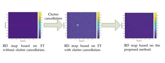
3. The Clutter Cancellation and Proposed Long Time Integration Algorithm

3.1. The Principle of Extensive Cancellation Algorithm

Unlike the traditional active radar, a reference antenna is required in passive radar for collecting the direct path signal that is transmitted by illuminators as the reference signal to accomplish the cross-correction. The surveillance antenna is mainly applied to capture the target echo; however, it is inevitably polluted by the direct-path and multipath signals. The strong clutter will degrade the target detection performance. Hence, it is critical to remove the clutter from the captured data before cross-correlation.
The sampled signal in surveillance channel is
s s u r v = [ s s u r v ( 0 ) s s u r v ( 1 ) s s u r v ( n ) s s u r v ( N 1 ) ] T
where N is the number of samples within the CPI.
Assuming that the clutter echoes are backscattered from the first R range cells, it is needed to extract the N + R 1 samples of the signal in reference channel:
s r e f = [ s r e f ( R + 1 ) s r e f ( 0 ) s r e f ( 1 ) s r e f ( n ) s r e f ( N 1 ) ] T
The signal model of ECA is for exploring by minimizing the residual signal power after clutter cancellation, thus
min α { s s u r v X α 2 }
with
X = B [ Λ P S r e f Λ 1 S r e f S r e f Λ 1 S r e f Λ P S r e f ]
where B is an incidence matrix that selects the last N rows of the matrix,
B = { b i j } i = 1 , , N   j = 1 , , N + R 1 ,   b i j = { 1 i = j R 1 0 o t h e r w i s e
Λ P is the diagonal matrix corresponding to the p-th Doppler cell.
S r e f = [ s r e f D s r e f D 2 s r e f D R 1 s r e f ]
where D is a 0/1 permutation matrix that applies a delay of a single sample that is defined as:
D = { d i j } i , j = 1 , , N + R 1 ,   d i j = { 1 i = j + 1 0 o t h e r w i s e
The columns of the matrix X define a M-dimensional clutter subspace, where M = ( 2 P + 1 ) R . The filter coefficients α = [ α 0   α 1     α R 1 ] T are evaluated based on the least square approach and it can be expressed as
α = ( X H X ) 1 X H s s u r v
The surveillance signal after clutter cancellation can be expressed as
s E C A = s s u r v X α = [ I N X ( X H X ) 1 X H ] s s u r v = P s s u r v
where P is the projection matrix projecting the surveillance channel signal in the subspace orthogonal to the clutter subspace.
After clutter cancellation, the received signals in surveillance channel are target echoes and thermal noise. Subsequently, cross-correlation and KT are applied to accomplish the range compression and range cell migrations, respectively.

3.2. The Proposed Long Time Integration Algorithm

It is worth noticing that DC and DRM that are related to the motion of the air target are constant during the CPI. The ratio of DRM and DC are defined as relative acceleration (RA), which can be expressed as
μ = f d m r f d c
Subsequently, (9) can be rewritten as
s ( t ^ m ) = A exp ( j 2 π λ ( R 0 + λ f d c t ^ m + 1 2 λ μ f d c t ^ m 2 ) ) = A exp ( j 2 π λ ( R 0 + λ f d c t ^ m ( 1 + 1 2 μ t ^ m 2 ) ) )
If the Doppler is constant during the CPI, FT can be applied to obtain the coherent integration processing gain. The target echo after cross-correlation and KT is denoted as S ( m , n ) , where m is the slow time and n is the fast time. We denote the range-Doppler map as I, the FT matrix as F, and the process of the coherent integration can be expressed as
I = F S
For a coherent integration containing M pulses, the FT matrix can be written as
F = W m m
where W = exp ( j 2 π M ) , m , m = 0 , 1 , 2 , , M 1 . Each m value corresponds to a row vector in the FT matrix. Subsequently, the integration component for quadratic phase terms in (20) can be expressed as
F c = W ( m M / 2 ) m μ / 2 / P R F
According to (23), the compensation component can be constructed with the variation of m and m . The size of the matrix F c is the same as F . The FT matrix containing the Doppler shift compensation is
F = F F c
where denotes Hadamard product and F is named as the long-time integration Fourier transform (LIFT) matrix. Subsequently, the coherent integration process can be expressed as
I = F S
The above analysis is based on the fact that the RA is already known. However, the ratio is unknown for the target and it needs to be estimated in advance.
Equation (9) indicates that the Doppler frequency can be described by a linear frequency modulated signal. Many parameter estimation methods can be applied to estimate the RA, such as fractional Fourier transform (FrFT) and Lv’s distribution [33,34]. Here, FrFT is used for parameter estimation. The definition of the FrFT for signal x ( t ) is
X p ( u ) = - x ( t ) K p ( u , t ) d t
K p ( u , t ) = { δ ( u t ) p = ( 2 n ± 1 ) π δ ( u t )   p = 2 n π   1 j cot p exp ( j π ( u 2 + t 2 ) cot p 2 u t csc p )   p n π
where K p ( u , t ) is the transform kernel that is defined as (27) and n = 1 , 2 . The result of the transformation concentrates the chirp signal energy on the specific point in the FrFT plane. Additionally, the parameters of the LFM signal can be obtained by
f ˜ d c = u csc p / T f ˜ d m r = ( c o t p ) . P R F T
Subsequently, the estimated RA can be calculated by
μ ˜ = f ˜ d m r / f ˜ d c = P R F cos p / u
However, the estimated value is inaccurate due to the interfere and noise. Here, we define a new variable to evaluate the coherent integration performance. The definition of energy integration ratio (EIR) is
ρ = E ( μ ˜ ) E
where E ( μ ˜ ) is the signal power of the Doppler cell that target located after coherent integration and E is the total signal power of the target echo after clutter cancellation. It can be noticed that ρ < 1 and a larger ρ indicates a better integration effect. Hence, the accurate μ ˜ can be obtained by maximizing the ρ .
Detailed implementation procedures of the proposed processing technique are given, as follows:
Step 1: Remove the direct and multipath signal from the target echo signal;
Step 2: Calculate the cross-correlation between the target echo signal and the reference signal;
Step 3: Estimate the coarse RA based on FrFT;
Step 4: Estimate the accurate RA through maximizing the EIR; and,
Step 5: Compensate the quadratic phase terms that are caused by the motion of the target and long time integration in the LIFT matrix.
In summary, Figure 3 illustrates the flowchart of the proposed processing technique.

4. Simulation Results and Discussion

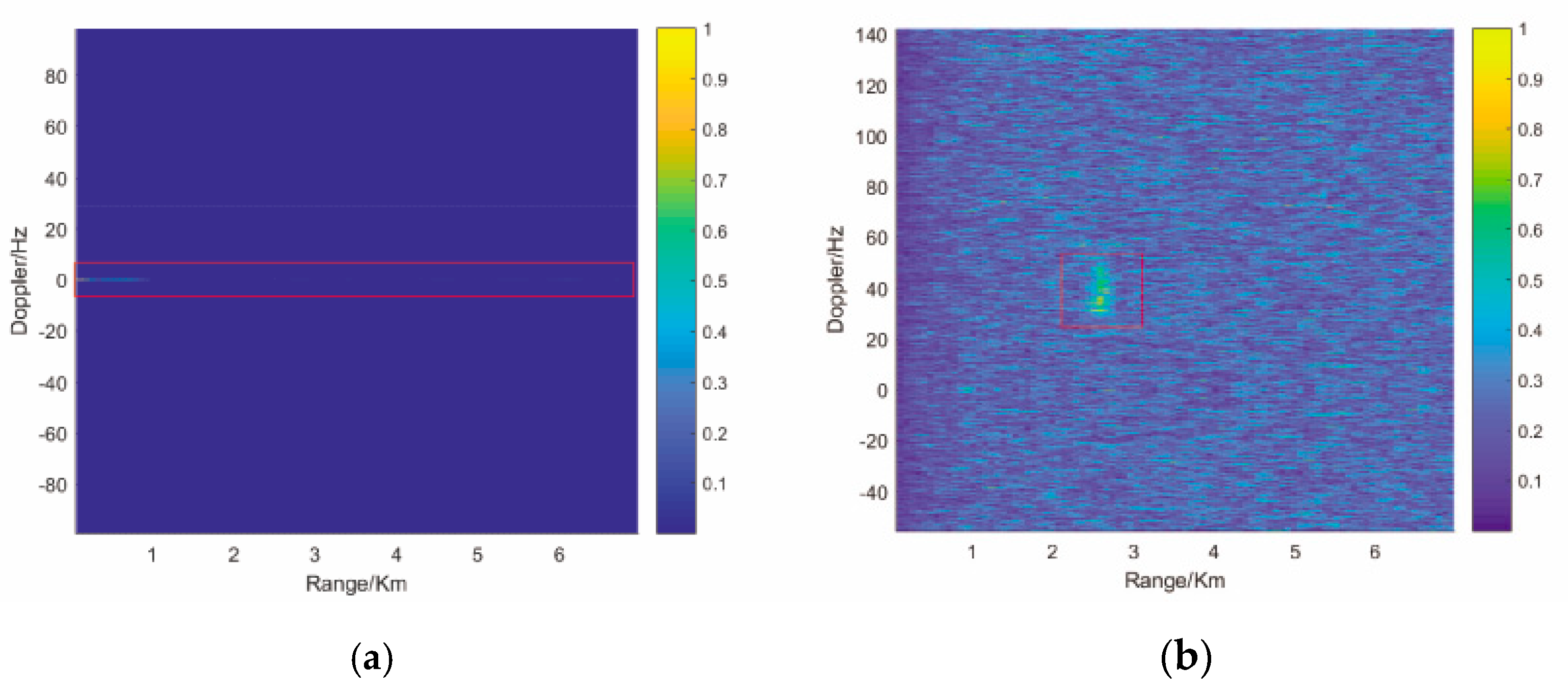
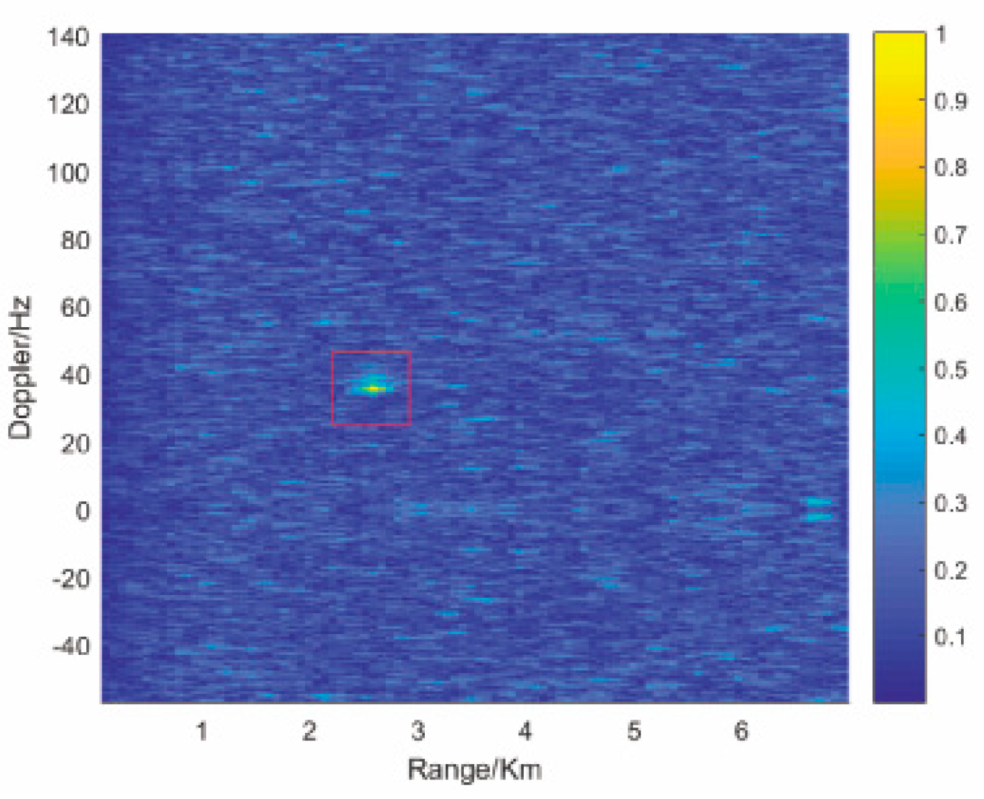
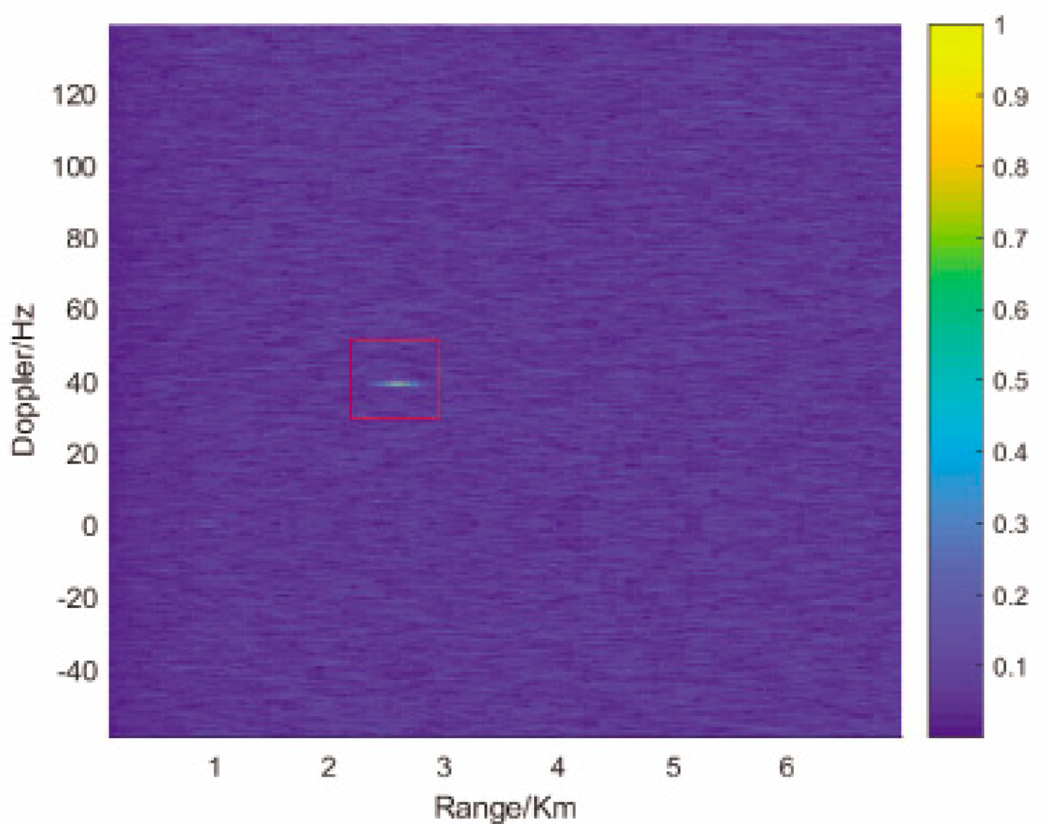
4.1. Simulation Results

In this section, the proposed method is tested by using MATLAB software to simulate the radar system and Table 1 provides the parameter settings of the radar system. The target echo pulses with different motion status are provided in order to verify the effectiveness of the proposed method.
In the simulation, GPS L1 signal is adopted as the transmitter of opportunity. The reason of this choice is that it represents the worst case in terms of signal power. The position of the satellite in the radar coordinate system is (5.59,7.19,18.2) × 106 m and its velocity is (60,100, −20) m/s. Two multipath signals are considered in the simulation. Table 2 illustrates the related parameters of the signals. When considering that Doppler frequency is related to the bistatic angle which is varying during the CPI, the coordinate form of Doppler frequency calculation is given here, as follows:
f d = 1 λ ( P T X P t P T X P t + P R X P t P R X P t ) [ v t x v t y v t z ]
where denotes the modular operation and [ v t x , v t y , v t z ] T is the target instantaneous velocity vector relative to the receiver.

4.1.1. Detection Results of Target with Smooth Motion

We consider the target with smooth motion and the acceleration is set as zero. At first, the conventional detection approach looking for the peak that the RD map got over a CPI is applied to detect the target. The RD map is obtained by performing a slow-time FT for the range-compressed echo. Figure 4 shows the RD map without considering the clutter cancellation. It can be seen that, except for the direct and multi-path echo located in zero Doppler, there is no bright spot that can be associated to the target. It can be deduced that the clutter and low power target echo affect the target detection performance.
Subsequently, we take clutter cancellation into consideration. Figure 5 shows the coherent processing results which both the direct and multipath signal at zero Doppler from the first 50 range cells (4400 m) are cancelled. Figure 5 provides the RD map obtained by the traditional FT. A clear spot that corresponds to the actual position of the target can be identified from Figure 5. However, the target energy has not been correctly gathered in the Doppler dimension due to the long integration time. The Doppler frequency of the target migrate several Doppler cells. When the echo signal is low, the target cannot be detected effectively. Moreover, the spread Doppler will affect the following parameter extraction.
Subsequently, the long time integration method that is based on modified radon Fourier transform (MFRT) is applied as comparison. Figure 6 shows the RD map obtained by MFRT. When compared with the RD map in Figure 5, it can be seen that the Doppler spread has been effectively eliminated. However, a slight spread is still existing in Doppler dimension. It can be deduced that the spread is caused by the parameter estimation error.
Next, the new proposed method is applied to deal with the data. Firstly, Figure 7a shows the instantaneous Doppler frequency versus the slow time. The red curve shown in Figure 7a is the real instantaneous Doppler frequency during the CPI, and the blue one is the result after curve fitting. It can be seen that the Doppler frequency is time varying and a slow-time FFT cannot effectively integrate the target energy. Figure 7b shows the errors between the real and fitting Doppler, from which it is seen that the errors are increased with the coherent integration time. The maximum error is 0.12 Doppler cell within the CPI, which can be negligible. It can also be noticed that the second-order expansion is sufficient for describing the Doppler variation during the dwell time.
Figure 8 is the parameter estimation result of signal in 33rd range cell by FrFT. The search interval of the rotation angle p was set to [ 0 , π ] with a step length of 0.005 π . The estimation result indicates that the DR and DMR are 3.14 and −56.12, respectively. The rough RA can be calculated according (21) and it is −0.056. The accurate RA is obtained by maximizing the EIR and the search interval is set to [ 0.066 , 0.046 ] , with a step length of 0.001. Figure 9 gives the EIR versus the RA, from which we can see that when the RA equals −0.061, the EIR is the largest. A more accurate RA can be obtained by a smaller step length, which means a longer computational time.
Figure 10 shows the coherent processing results obtained by the proposed processing technique. It can be seen from Figure 10 that the target energy is correctly accumulated over the CPI. As evident, a bright spot that is well-gathered in both range and Doppler dimensions can be noticed in the RD map, and the Doppler spreads in Figure 5 and Figure 6 have been eliminated effectively.
Figure 11 presents the Doppler cross-section of 33rd range cell to further illustrate the effectiveness of the new proposed method. As is apparent, the new proposed method has effectively integrated the signal energy during the long dwell time. A clear peak can be individuated in the red curve. Specifically, it is seen that an improvement of more than 10 dB is obtained. Such an improvement indicates the effectiveness and robustness of the proposed processing technique.

4.1.2. Detection Results of Target with Constant Acceleration

Usually, the motion of the air target is not smooth, and the acceleration must be considered. In this section, the proposed technique is tested by the target with constant acceleration. We set the acceleration of the target as (−3, −5, 1) m/s2, while the velocity and initial position of the target remain unchanged. The SNR of the target echo is set as −46 dB. ECA cancels the clutter from the first 50 range cells.
Figure 12a is the detection result that is based on FT without clutter cancellation. As can be seen, the target cannot be identified due to the strong direct and multipath signals. Figure 12b provides the RD map obtained by FT with clutter cancellation, from which we can see that the target echo has not been accumulated effectively. Although the target can be identified in the RD map, the Doppler spans several resolution cells. Figure 13 shows an RD map obtained by the MFRT. The target echoes have been gathered and a bright spot can be identified in the map. However, the Doppler spread has not been eliminated effectively.
Figure 14a is the Doppler variation during the CPI. When comparing with Figure 7a, the Doppler changes more severely due to the maneuvering of the target. The maximum curve fitting error is 1.8 Doppler cells and it can be negligible in the subsequent processing.
Next, the proposed processing technique is applied to obtain a high coherent integration gain. The coarse RA that is estimated by FrFT is −0.0079. The accurate RA is obtained by maximizing the EIR and the search interval is set to [ 0.089 , 0.069 ] , with a step length of 0.001. The running results indicate that, when the RA equals −0.0083, the EIR achieves maximum.
The signal to background ratio has been improved due to the enhanced energy concentration by the proposed method. The RD map that is given in Figure 15 also indicates that the target echoes have been accumulated in both range and Doppler dimensions. A bright spot can be identified in the RD map.
When compared with the traditional target detection method, the proposed method can obtain a higher coherent integration gain, and a longer detection range is guaranteed. Both of the the simulation results presented above indicate the effectiveness of the proposed processing technique.

4.2. Discussion

In this part, the system link budget will be analyzed. Investigating the maximum detection range of this system as a function of the coherent integration time is the main objective of this analysis.
According to the bistatic radar function, the SNR for the echo signal is
S N R i n = ρ G r λ 2 σ η ( 4 π ) 2 R R 2 P n
where Table 3 provides the parameters of the radar system. Next, we take the signal processing gain into consideration. The whole signal processing gain G s p can be written as:
G s p = B T c T c o h T c
where B T c and T c o h T c , respectively, denote the range and azimuth processing gain. After the two-dimensional integration processing, the SNR of the echo signal is:
S N R o u t = S N R i n G s p = ρ G r λ 2 σ η ( 4 π ) 2 R R 2 P n B T c o h
We set the minimum SNR for the target detection is S N R min = 8   dB and the coherent time T c o h = 3   s . Subsequently, the detection of the GNSS_based passive radar system is 3.5 km.
A large-scale antenna with long integration interval is highly recommended to further enhance the detection range of the GNSS_based radar system. Moreover, any point on the earth is illuminated by more than 32 satellites simultaneously, the detection range can also be enhanced by utilizing multiple satellites. Research on the exploitation of multiple satellites to increase the detection range is our future work.

5. Conclusions

In this paper, we address the detection of air targets by means of the passive bistatic radar that is based on low-EIRP GPS satellite. Extensive cancellation algorithm (ECA) which project the surveillance channel signal in the subspace orthogonal to the clutter subspace is firstly applied in GNSS-based bistatic radar. Subsequently, a new coherent processing method that is based on LIFT is proposed for long time integration. The parameter, RA, is defined to describe the Doppler variation during the dwell time. Based on RA, the quadratic phase terms that are caused by the longtime integration can be compensated in the LIFT matrix. A rough estimation of RA is obtained by FrFT and an accurate one is obtained through the optimal detection results. The proposed method can effectively accumulate the target echo during the CPI when compared with the traditional integration method. Simulation experiments verify the excellent performance of the proposed processing method. Our future work focuses on the targets with complex motion and explores the target detection and tracking under low SNR.

Author Contributions

Conceptualization, B.W. and Z.Z.; methodology, B.W.; software, B.W.; validation, B.W.; writing—original draft preparation, B.W.; writing—review and editing, H.C., Z.Z. and B.T.; visualization, B.W.; supervision, H.C.; project administration, B.T.; funding acquisition, B.T. All authors have read and agreed to the published version of the manuscript.

Funding

This research was funded by National Natural Science Foundation of China grant number 41975005.

Institutional Review Board Statement

Not applicable.

Informed Consent Statement

Not applicable.

Data Availability Statement

Not applicable.

Acknowledgments

The authors would like to thank the editors and the reviewers for their valuable suggestions.

Conflicts of Interest

The authors declare no conflict of interest.

Abbreviations

The following abbreviations are used in this manuscript:
GNSSglobal navigation satellite system
ECAextensive cancellation algorithm
LIFTlong-time integration Fourier transform
RArelative acceleration
PBRpassive bistatic radar
LMSleast mean square
NLMSnormalized least mean square
RLSrecursive least square
LSleast square
EIRPeffective isotropic radiated power
CPIcoherent processing interval
FrFTfractional Fourier transform
SNRsignal to noise ratio
DCDoppler centroid
DMRDoppler modulated rate
FTFourier transform
EIRenergy integration ratio
RDrange Doppler

References

  1. Zeng, H.; Chen, J.; Wang, P.; Liu, W.; Zhou, X.; Yang, W. Moving Target Detection in Multi-Static GNSS-Based Passive Radar Based on Multi-Bernoulli Filter. Remote Sens. 2020, 12, 3495. [Google Scholar]
  2. He, Z.-Y.; Yang, Y.; Chen, W.; Weng, D.-J. Moving Target Imaging Using GNSS-Based Passive Bistatic Synthetic Aperture Radar. Remote Sens. 2020, 12, 3356. [Google Scholar]
  3. Hu, C.; Liu, C.; Wang, R.; Chen, L.; Wang, L. Detection and SISAR Imaging of Aircrafts Using GNSS Forward Scatter Radar: Signal Modeling and Experimental Validation. IEEE Trans. Aerosp. Electr. Syst. 2017, 53, 2077–2093. [Google Scholar]
  4. Noviello, C.; Esposito, G.; Fasano, G.; Renga, A.; Soldovieri, F.; Catapano, I. Small-UAV Radar Imaging System Performance with GPS and CDGPS Based Motion Compensation. Remote Sens. 2020, 12, 3463. [Google Scholar]
  5. Wang, Y.; Bao, Q.; Wang, D.; Chen, Z. An Experimental Study of Passive Bistatic Radar Using Uncooperative Radar as a Transmitter. IEEE Geosci. Remote Sens. Lett. 2015, 12, 1868–1872. [Google Scholar]
  6. Zeng, H.; Wang, P.; Chen, J.; Liu, W.; Ge, L. A Novel General Imaging Formation Algorithm for GNSS-Based Bistatic SAR. Sensors 2016, 16, 1–15. [Google Scholar]
  7. Colone, F.; Bongioanni, C.; Lombardo, P. Multifrequency integration in FM radio-based passive bistatic radar. Part I: Target detection. IEEE Aerosp. Electr. Syst. Mag. 2013, 28, 28–39. [Google Scholar]
  8. Malanowski, M.; Kulpa, K.; Kulpa, J.; Samczynski, P.; Misiurewicz, J. Analysis of detection range of FM-based passive radar. IET Radar Sonar Navig. 2014, 8, 153–159. [Google Scholar]
  9. Howland, P.; Maksimiuk, D.E.; Reitsma, G. FM radio based bistatic radar. Proc.-Radar Sonar Navig. 2005, 152, 107–115. [Google Scholar]
  10. Martelli, T.; Colone, F.; Tilli, E.; di Lallo, A. Multi-frequency target detection techniques for DVB-T based passive radars sensors. Sensors 2016, 10, 1594. [Google Scholar] [CrossRef] [Green Version]
  11. Griffiths, H.D.; Long, N.R.W. Television-based Bistatic Radar. IEE Proc. F Commun. Radar Signal Process. 1986, 133, 649–657. [Google Scholar]
  12. Guo, H.; Woodbridge, K.; Baker, C.J. Evaluation of WIFI Beacon Transmissions for Wireless Based Passive R adar. In Proceedings of the 2008 IEEE Radar Conference, Rome, Italy, 26–30 May 2008; pp. 1–6. [Google Scholar]
  13. Colone, F.; Falcone, P.; Bongioanni, C.; Long, P.L. WiFi-based passive bistatic radar: Data processing schemes and experimental results. IEEE Trans. Aerosp. Electr. Syst. 2012, 48, 1061–1079. [Google Scholar]
  14. Zemmari, R.; Broetje, M.; Battistello, G.; Nickel, U. GSM passive coherent location system: Performance prediction and measurement evaluation. IET Radar Sonar Navig. 2014, 8, 94–105. [Google Scholar]
  15. Ma, H.; Antoniou, M.; Pastina, D.; Santi, F.; Pieralice, F.; Bucciarelli, M.; Cherniakov, M. Maritime moving target indication using passive GNSS-based bistatic radar. IEEE Trans. Aerosp. Electr. Syst. 2018, 54, 115–130. [Google Scholar]
  16. Hui, M.; Michail, A.; Stove, A.G.; Winkel, J.; Cherniakov, M. Maritime Moving Target Localization Using Passive GNSS-Based Multistatic Radar. IEEE Trans. Geosci. Remote Sens. 2018, 56, 4808–4819. [Google Scholar]
  17. Pastina, D.; Santi, F.; Pieralice, F.; Bucciarelli, M.; Ma, H.; Tzagkas, D.; Antoniou, M.N.; Cherniakov, M. Maritime moving target long time integration for GNSS-based passive bistatic radar. IEEE Trans. Aerosp. Electr. Syst. 2018, 6, 1–12. [Google Scholar]
  18. Tan, D.K.P.; Lesturgie, M.; Sun, H.; Lu, Y. Space time interference analysis and suppression for airborne passive radar using transmissions of opportunity. IET Radar Sonar Navig. 2014, 8, 142–152. [Google Scholar]
  19. Ma, Y.; Shan, T.; Zhang, Y.D.; Amin, M.G.; Tao, R.; Feng, Y. A novel two-dimensional sparse-weight NLMS filtering scheme for passive bistatic radar. IEEE Geosci. Remote Sens. Lett. 2016, 13, 676–680. [Google Scholar]
  20. Zhu, X.-L.; Zhang, X.-D. Adaptive RLS algorithm for blind source separation using a natural gradient. IEEE Signal Process. Lett. 2002, 9, 432–435. [Google Scholar]
  21. Colone, F.; O’Hagan, D.W.; Lombardo, P.; Baker, C.J. A Multistage Processing Algorithm for Disturbance Removal and Target Detection in Passive Bistatic Radar. IEEE Trans. Aerosp. Electr. Syst. 2009, 45, 698–722. [Google Scholar]
  22. Colone, F.; Palmarini, C.; Martelli, T.; Tilli, E. Sliding extensive cancellation algorithm for disturbance removal in passive radar. IEEE Trans. Aerosp. Electron. Syst. 2016, 52, 1309–1326. [Google Scholar]
  23. Zhao, Z.; Zhou, X.; Zhu, S.; Hong, S. Reduced complexity multipath clutter rejection approach for DRM-based HF passive bistatic radar. IEEE Access 2017, 5, 20228–20234. [Google Scholar]
  24. Rohman, P.A.; Nishimoto, M. Ground clutter suppression in GPR using framing based mean removal and subspace decomposition. In Proceedings of the 2017 International Symposium on Antennas and Propagation (ISAP), Phuket, Thailand, 30 October–2 November 2017; pp. 1–2. [Google Scholar]
  25. Cardillo, E.; Li, C.; Caddemi, A. Vital Sign Detection and Radar Self-Motion Cancellation Through Clutter Identification. IEEE Trans. Microw. Theory Tech. 2021. [Google Scholar] [CrossRef]
  26. Zeng, H.-C.; Chen, J.; Wang, P.-B.; Yang, W.; Liu, W. 2-D Coherent Integration Processing and Detecting of Aircrafts Using GNSS-Based Passive Radar. Remote Sens. 2018, 99, 1164. [Google Scholar]
  27. Tao, R.; Deng, B.; Wang, Y. Research progress of the fractional Fourier transform in signal processing. Sci. China Inf. Sci. 2006, 49, 1–25. [Google Scholar]
  28. Xu, J.; Yan, L.; Zhou, X.; Long, T.; Xia, X.-G.; Wang, Y.-L.; Farina, A.; Xai, X.-G. Adaptive Radon-Fourier Transform for Weak Radar Target Detection. IEEE Trans. Aerosp. Electr. Syst. 2018, 99, 686–697. [Google Scholar]
  29. He, Z.; Yang, Y.; Chen, W. A Hybrid integration method for moving target detection with GNSS-based passive radar. IEEE J. Sel. Top. Appl. Earth Obs. Remote Sens. 2020, 99, 1. [Google Scholar]
  30. Li, Z.; Santi, F.; Pastina, D.; Lombardo, P. Passive Radar Array with Low-Power Satellite Illuminators Based on Fractional Fourier Transform. IEEE Sens. J. 2017, 17, 8378–8394. [Google Scholar]
  31. Zhou, X.; Wang, P.; Chen, J.; Men, Z.; Liu, W.; Zeng, H.A. Modified Radon Fourier Transform for GNSS-Based Bistatic Radar Target Detection. IEEE Geosci. Remote Sens. Lett. 2020, 1–5. [Google Scholar] [CrossRef]
  32. Perry, R.P.; DiPietro, R.C.; Fante, R.L. SAR imaging of moving targets. IEEE Trans. Aerosp. Electron. Syst. 1999, 35, 188–200. [Google Scholar]
  33. Lv, X.; Bi, G.; Wan, C.; Xing, M. Lv’s distribution: Principle, implementation, properties, and performance. IEEE Trans. Signal Process. 2011, 59, 3576–3591. [Google Scholar]
  34. Li, X.; Cui, G.; Yi, W.; Kong, L. Coherent Integration for Maneuvering Target Detection Based on Radon-Lv’s Distribution. IEEE Signal Process. Lett. 2015, 22, 1467–1471. [Google Scholar]
Figure 1. Geometric configuration of Global Navigation Satellite Systems_based (GNSS_based) bistatic radar.
Remotesensing 13 00701 g001
Figure 2. Two-dimensional rearranged data.
Remotesensing 13 00701 g002
Figure 3. Flowchart of the new imaging approach.
Remotesensing 13 00701 g003
Figure 4. RD map based on Fourier transform (FT) without clutter cancellation.
Remotesensing 13 00701 g004
Figure 5. RD map based on FT with clutter cancellation.
Remotesensing 13 00701 g005
Figure 6. RD map based on modified radon Fourier transform (MFRT).
Remotesensing 13 00701 g006
Figure 7. Doppler variation during the coherent processing interval (CPI). (a) Doppler variation and curve fitting result. (b) Curve fitting error.
Remotesensing 13 00701 g007
Figure 8. Fractional Fourier transform (FrFT) result of the 33rd range cell.
Remotesensing 13 00701 g008
Figure 9. Energy integration ratio (EIR) versus the RA.
Remotesensing 13 00701 g009
Figure 10. Coherent processing results based on the proposed method.
Remotesensing 13 00701 g010
Figure 11. Doppler cross-section of the target.
Remotesensing 13 00701 g011
Figure 12. Coherent processing results based on FT. (a) Detection result without clutter cancellation. (b) Detection result with clutter cancellation.
Remotesensing 13 00701 g012
Figure 13. RD map based on MFRT.
Remotesensing 13 00701 g013
Figure 14. Doppler variation during the CPI. (a) Doppler variation and curve fitting result. (b) Curve fitting error.
Remotesensing 13 00701 g014
Figure 15. Coherent processing results based on the proposed method.
Remotesensing 13 00701 g015
Table 1. Parameters of the radar system.
ParameterSetting ValueParameterSetting Value
Carrier frequency1575.42 MHzBandwidth1.023 MHz
Complex sampling rate4.092 MHzPulse repeat frequency1000 Hz
Pulse number3000Range resolution146.6 m
Table 2. Related simulation parameter.
ParameterSNR (dB)Sample Delay
Direct signal00
Multipath 1−7.965
Multipath 2−6.029
Target echo−4033
Table 3. System link budget parameter.
ParameterSymbolSetting Value
Power density ρ −158 dBw
Wavelength λ 0.19 m
Code duration T c 1 ms
Code bandwidth B 1.023 MHz
Receiver antenna gain G r 35 dB
RCS σ 20 dB
Noise power P n −143 dB
System loss factor η 0.5
Coherent time T c o h 3 s
Publisher’s Note: MDPI stays neutral with regard to jurisdictional claims in published maps and institutional affiliations.

