Abstract
Atmospheric compensation (AC) allows the retrieval of the reflectance from the measured at-sensor radiance and is a fundamental and critical task for the quantitative exploitation of hyperspectral data. Recently, a learning-based (LB) approach, named LBAC, has been proposed for the AC of airborne hyperspectral data in the visible and near-infrared (VNIR) spectral range. LBAC makes use of a parametric regression function whose parameters are learned by a strategy based on synthetic data that accounts for (1) a physics-based model for the radiative transfer, (2) the variability of the surface reflectance spectra, and (3) the effects of random noise and spectral miscalibration errors. In this work we extend LBAC with respect to two different aspects: (1) the platform for data acquisition and (2) the spectral range covered by the sensor. Particularly, we propose the extension of LBAC to spaceborne hyperspectral sensors operating in the VNIR and short-wave infrared (SWIR) portion of the electromagnetic spectrum. We specifically refer to the sensor of the PRISMA (PRecursore IperSpettrale della Missione Applicativa) mission, and the recent Earth Observation mission of the Italian Space Agency that offers a great opportunity to improve the knowledge on the scientific and commercial applications of spaceborne hyperspectral data. In addition, we introduce a curve fitting-based procedure for the estimation of column water vapor content of the atmosphere that directly exploits the reflectance data provided by LBAC. Results obtained on four different PRISMA hyperspectral images are presented and discussed.
1. Introduction
Hyperspectral sensors (HSs) offer the opportunity of analyzing the chemical and physical composition of the remote sensed scene thanks to their ability of measuring the spectrum of the observed pixels in a large number of contiguous and narrow spectral channels [1]. In particular, spaceborne sensors allow the exploitation of the potential of hyperspectral technology for large-scale monitoring of the earth [2]. The set of Earth Observation (EO) applications enabled by spaceborne HSs includes [3,4,5,6] detailed environmental monitoring, forest analysis, precision agriculture, inland and coastal water monitoring, raw material exploration and mining, soil degradation, and analysis.
Despite the technological advances, hyperspectral satellites are still poorly represented in spaceborne missions compared to multispectral ones [2]. In this context, the Italian Space Agency (ASI) EO mission named PRISMA (PRecursore IperSpettrale della Missione Applicativa, [7,8,9,10]) offers a great opportunity to improve the knowledge about the scientific and commercial applications of spaceborne hyperspectral data. PRISMA, launched in March 2019 [11], includes a pushbroom hyperspectral camera covering the portion of the electromagnetic spectrum ranging from 400 nm to 2500 nm with 10 nm spectral sampling. Specifically, the hyperspectral sensor is composed of two partially overlapped spectrometers operating in the Visible, Near InfraRed (VNIR), and ShortWave InfraRed (SWIR) spectral ranges, respectively [10]. The sensor acquires scenes of 30 km × 30 km with a Ground Sampling Distance (GSD) of 30 m.
One of the critical issues in the exploitation of hyperspectral remotely sensed data is represented by the distortion effects due to the atmosphere in the radiative transfer path [12]. The information about the composition of the observed material is contained in its spectral reflectance. Remote sensing sensors measure the at-sensor spectral radiance that can be considered as an altered version of the spectral reflectance where distortion is due to the effects of the solar illumination and the atmosphere composition. To derive the spectral reflectance of the observed material, those effects must be properly compensated by means of a process called Atmospheric Compensation (AC, [13,14,15,16]. In the VNIR-SWIR spectral range, atmospheric effects mostly depend on [13,14,15] (a) the absorption of water vapor, (b) the aerosol extinction, and (c) the absorption of uniformly mixed gases such as oxygen (O2), ozone (O3), carbon dioxide (CO2) and methane (CH4).
The most effective and reliable approach to the AC of hyperspectral data is the Physics-based (PB) one [13,14,15,16,17,18] that exploits an analytical model of the radiative transfer in the atmosphere (Radiative Transfer Model-RTM). PB methods follow a common approach [14] where, first the parameters characterizing the atmosphere (mainly the visibility and the column water vapor concentration ) are estimated from the available data, and then the spectral radiometric quantities in the adopted RTM are derived by means of a specific radiative transfer code (e.g., Modtran [19], and, finally, the spectral reflectance of each image pixel is derived by inverting the RTM. Often, to remove the effects of random noise and miscalibration artifacts from atmospherically compensated data, they are processed by means of a filtering procedure generally known as spectral polishing [16].
In a recently published work [20], a new approach for AC of VNIR hyperspectral data was introduced. It is called the learning-based atmospheric compensation (LBAC) approach and makes use of machine learning methods to directly estimate the spectral reflectance from the at-sensor radiance accounting for the variability induced by one or more unknown parameters of the RTM and by-passing their estimation. Specifically, LBAC derives the spectral reflectance from the at-sensor spectral radiance by means of a parametric regression function whose parameters are determined through a specific learning strategy that exploits simulated data to account for the variability of both the atmosphere and the surface spectral reflectance. The learning strategy is specifically designed to take noise into account in order to make the regression function robust to its effects. The approach introduced in [20] is quite general and different types of parametric regression functions can be used, including those characterized by complex architectures such as deep neural networks. In [20], a first parametric function based on multilinear regression was tested on real airborne hyperspectral data acquired in the VNIR spectral range and several results were presented and discussed along with an extensive analysis over simulated data.
In this work, we focus on the extension of the previous analysis of LBAC results in two directions: (a) we consider hyperspectral data acquired from a spaceborne platform, and (b) we consider an extended spectral range including the SWIR, where the atmosphere has stronger water absorption windows than those in the VNIR spectral region. It is worth noting that, though the LBAC algorithm considered in this work uses the same regression model proposed in [20], the parameter matrix that defines the specific regression function is changed both in terms of cardinality and values. Such a matrix is obtained in the learning phase using a training set that differs from that in [20] for two main aspects. First, the training set is here obtained by simulating the atmospheric effects in the SWIR spectral range and not only in the VNIR spectral range. Then, in order to account for satellite acquisition conditions, atmospheric layers up to an altitude of 100 km have been considered and the description of the acquisition geometry has been enriched with the inclusion of the sensor viewing angle and the relative azimuth angle between the incident solar direction and the direction of propagation of the scattered radiance. In this work, we refer to the PRISMA data domain, and, for this purpose, we analyze images acquired by the hyperspectral camera of the PRISMA mission. In addition, we propose a retrieval algorithm that exploits LBAC outputs in combination with a curve fitting approach to obtain per-pixel estimates of from PRISMA radiance data. It is worth noting that here we focus on the extension of the LBAC method to the specific case of modern spaceborne hyperspectral missions with particular reference to the PRISMA mission. The reader is referred to [20] for the detailed description of the LBAC procedure.
This paper is organized as follows. In Section 2 we summarize the LBAC algorithm and provide implementation details for its extension to spaceborne sensors and to the SWIR spectral range. In Section 3, we introduce the procedure that exploits LBAC outputs for the estimation of values in each image pixel. Finally, in Section 4, we present and discuss results obtained by applying the LBAC to real PRISMA images.
2. LBAC Algorithm
The LBAC algorithm applied to VNIR-SWIR satellite hyperspectral data is based on the following RTM [15]. Denoted by as the at-sensor radiance vector (where is the number of sensor channels), and assuming a Lambertian model for the description of the observed surface, can be expressed as:
where is the solar zenith angle and denotes the ground reflected radiance, i.e., the contribution of the solar radiation that after the interaction with the surface is captured by the sensor. The description of the radiometric quantities in Equation (1) is summarized in Table 1 We assume that the vector of the spectral radiance from adjacent regions is available and modelled as [15,18]. For the sake of conciseness, in Equation (1) the parameters specifying the acquisition conditions (acquisition geometry and atmosphere) are grouped in the vector .

Table 1.
Description of the radiometric quantities in Equation (1).
On the basis of the smooth behavior observed in the spectral reflectance of most of the natural and artificial materials [16,21], the vector is assumed as lying into a vector subspace with rank lower than that of the original data space (. Thus, it can be expressed as with denoting one of the possible basis matrices of the above-mentioned subspace. In the derivation of LBAC [20], is obtained by applying a procedure based on Singular Value Decomposition to the data of a spectral reflectance library . The spectral library contains more than 3000 measured spectral reflectances of several artificial materials, vegetation, water, soils, and minerals and it was obtained by merging three available spectral libraries: ASTER (Advanced Spaceborne Thermal Emission Reflection Radiometer, [22], USGS (United States Geological Survey-version released in 2007, [23] and ANGERS [24].
LBAC estimates directly from the at-sensor radiance of the observed pixel and that from adjacent regions regardless of the spatially varying values of , and without the calculation of the radiometric quantities. The only atmospheric parameter to be estimated is . is, generally, obtained from the analyzed data [13,18] by applying a linear and space invariant filter whose impulse response approximates the atmospheric Point Spread Function (PSF). In the implementation of the LBAC algorithm we use the impulse response proposed in [25].
Specifically, for each image pixel, LBAC receives and as input and provides as output the estimates of the vector components and of the spectral reflectance of the observed surface. The output is obtained by means of a multiple linear regression function:
The parameter matrix . is obtained by means of a specific learning strategy that minimizes the following loss function:
where and . denote the -norm and the Frobenius norm, respectively.
The learning strategy exploits a training set of simulated triplets generated according to the RTM in Equation (1). The simulation strategy uses Modtran to generate the radiometric quantities in Equation (1) and the spectral library for the generation of the spectral reflectance of the observed surface and of its adjacent surfaces. These are generated by applying the Linear Mixture Model to randomly selected elements of . Both the selected spectra and the mixing coefficients are randomly chosen [20].
In simulating the training sample for the learning phase, the Modtran parameter related to is randomly varied according to a uniform distribution in the range . The rest of the Modtran parameters are kept constant. We refer to: (a) the parameters MODEL and IHAZE that specify the geographical and seasonal model and the aerosol model; (b) the visibility ; (c) the total column amounts of O2, O3, CO2, and CH4. As to the parameters related to the acquisition geometry, in [20], with reference to typical airborne applications, the sensor height and the solar zenith angle () were considered. Here, referring to spaceborne applications, the height of the sensor is irrelevant (all the atmospheric layers included in Modtran are considered) and the acquisition geometry is defined by , the sensor viewing angle () and the relative azimuth angle between the incident solar direction and the direction of propagation of the scattered radiance ().
Various regression functions are trained by varying the above-mentioned parameters. In this work, for the parameters MODEL, IHAZE, and we consider the same values as in [20]. For we consider values in the range [0,180] deg with a step of 20 deg and for , values in the range [−21,21] deg with a step of 1 deg. The extremes of the latter range are in accordance with the maximum off-nadir pointing of the PRISMA mission [10]. For the total column amounts of O2, O3, CO2, and CH4., we consider the default Modtran values determined by the parameter MODEL. Notice that the regressors applied to a given hyperspectral image, are chosen from the set of all the trained regressors on the basis of the specific a priori known acquisition conditions (geographical area, acquisition date, and time, and acquisition geometry).
It is worth noting that, in order to apply LBAC to the PRISMA data, the general architecture of the algorithm has not been modified with respect to that proposed in [20] and recalled in Equation (2). What is actually changed is the simulation of the training set which also takes into account the effects of the atmosphere in the SWIR spectral range. Of course, the simulated training sets are mapped in the sensor spectral domain by accounting for the specific Spectral Response Function of the sensor channels of the PRISMA hyperspectral sensor.
One of the advantages offered by LBAC is its robustness to spectral mis-calibration errors and random noise, which is achieved by considering such sources of disturbance in the algorithm training phase. Noise has been simulated according to the realistic signal-dependent noise model described in [26,27]. In simulating the training set, noise realizations are added to radiance vectors with different values of the Signal to Noise Ratio (SNR) drawn from a uniform distribution in the range . The current version of the LBAC algorithm does not account for the effects of terrain elevation.
2.1. Visibility Estimation
LBAC assumes the knowledge of the parameter that is fundamental for selecting the specific regression model to be used. In practice, the value of is not known and must be estimated from the analyzed image. In [20], an estimation method was proposed based on dark pixels analysis [28]. It relies on the assumption that, denoted as a certain set of bands not affected by water vapor and gases absorption, the image contains, for each band in , at least one pixel where the contribution of the ground reflected radiance () is negligible.
Denoting with , the vector of the darkest value of the image in each band of , it can be viewed as an approximation of the upwelling atmospheric spectral radiance , which depends on the specific acquisition conditions of the analyzed image and, in particular, on . The above-mentioned approximation is compared with a Look-Up Table (LUT) of vectors simulated by Modtran for different values of , to obtain the estimate of the visibility.
In this work, the algorithm in [20] has been modified in some of its parts for the extension to satellite data.
Firstly, the algorithm proposed in [20], was designed for airborne applications (small scene) and provides a single visibility estimate for the entire image. In the case of PRISMA data, given the spatial extent of the observed scene (30 km × 30 km), constant visibility is unlikely to occur. Thus, the visibility estimation algorithm is applied locally by considering non-overlapping image patches of 20 × 20 pixels (600 m × 600 m). This choice is in line with the strategy adopted by the PRISMA L2C data processor as reported in [29].
Furthermore, different algorithms are applied to land and water areas on the basis of a pre-classification of the entire image. Specifically, for land areas, includes the first 32 channels of the PRISMA hyperspectral sensor corresponding to the central wavelengths in the range . For water areas, is the set of all the bands with central wavelengths above 650 nm not affected by water and gases (O2, CO2, and CH4) absorption. The latter choice is motivated by the fact that water-leaving reflectance is almost zero in the near- and short-wave infrared spectral range.
In the case of land areas, where the probability of occurrence of dark pixels is generally low, is obtained by averaging the 10 darkest pixels detected in that region of the image. For water areas, a greater number of samples can be considered to estimate the visibility. Thus, is obtained by averaging all the water pixels in the selected image region in order to mitigate noise effects.
In both cases, visibility is estimated by minimizing, with respect to , the following loss function:
where is the vector of RTM parameters excluding , is the number of bands in and is the Heaviside step function. The first term in Equation (4) measures the relative distance between and , while the second term accounts for the physical non-negative constraint . The minimization of the function in Equation (4) is carried out by considering values of ranging from 10 km to 100 km.
It is worth noting that the dark pixel method, when applied to land images, provides good results in the region containing shadowed pixels, dark vegetation pixels or, in general, low reflectance pixels (at least in the set of bands ). It tends to underestimate in image sub-regions where all the pixels correspond to bright materials (e.g., desert areas). To mitigate the underestimation of , after the local estimation procedure, a 3 × 3 bidimensional median filter is applied to the resulting visibility estimation matrix to filter out potential outliers. Values of the estimated visibility lower than 10 km are discarded and replaced by the average visibility obtained in the rest of the image pixels. This strategy is similar to that adopted by other methods proposed in the literature and based on dark pixels.
Notice that, in land-water transition patches (e.g., those corresponding to coastal regions), visibility is estimated by considering the procedure designed for water pixels.
It is worth stressing that, as opposed to water vapor, that has absorption effects characterized by distinctive spectral shapes over narrow intervals, atmospheric aerosols determine spectrally smooth perturbations that can be difficult to disentangle from changes in surface reflectance. Despite the recent advances in AC methods, estimating visibility remains an open and challenging problem [16]. Algorithms that work well under all the possible conditions are not currently available [16].
One possible way to tackle this problem is to involve in the visibility estimation process aerosol thickness products from other satellite missions specifically conceived for this purpose (e.g., Sentinel 3 L2 [30], Terra/Modis [31].
3. CWV Retrieval Based on LBAC Results
LBAC is specifically conceived to retrieve the surface spectral reflectance regardless of the values in the atmosphere. It does not require the estimates of the atmospheric parameters as input. However, in some EO applications, it is important to estimate , because it is a tracer for tropospheric changes, and it is important for climate prediction and global circulation models determination [32]. For this reason, we have developed a new algorithm that exploits the reflectance obtained by LBAC (regardless of the values) to estimate . Such a strategy is opposite to those adopted in traditional AC algorithms that perform estimations as a preliminary step for RTM model inversion. Common methods for retrieval is the Atmospheric Pre-corrected Differential Absorption algorithm (APDA, [29] and the curve fitting techniques [15,33]. APDA exploits the at-sensor radiance values in three groups of channels: the measurement channels with a spectral central wavelength falling within an atmospheric water vapor absorption region (typically around 820 nm or 940 nm), and two “reference” channels corresponding to the wavelengths located at each side of the water absorption band where absorption due to CWV is almost negligible. Those at-sensor radiance data are combined to compute the “depth” of the absorption feature that is related to CWV. The computed “depth” is compared with a pre-calculated look-up table to obtain the estimate of the CWV parameter. APDA makes use of the simplifying hypothesis that the spectral reflectance in the measurement channel has a fixed value (0.4) regardless of the observed surface.
Spectral curve fitting [33] is an alternative approach that searches for the best match between the radiance measured in the water absorption bands and that generated according to the RTM by assuming the spectral reflectance in those bands as linearly dependent on the wavelengths. In reality, the reflectance is never a perfect linear continuum; more complex surface reflectance shapes can distort both ratios and spectral fits. To deal with this problem, in [15] a low-rank approximation of the spectral reflectance in the water absorption band was proposed.
In this work, we propose a curve fitting approach where the reflectance values in the considered water absorption bands are those provided by the LBAC algorithms. Specifically, denoting as a set of sensor channels falling in the water absorption bands, a estimate for each image pixel is obtained as the minimum of the following loss function:
where and are, respectively, the estimate of the spectral reflectance provided by the LBAC, and the estimate of the visibility given by the procedure in Section 2.1 in the region of the image comprising the pixel under consideration. The superscript indicates that the vectors and are considered in the spectral channels included in . and are the measured and the RTM derived at-sensor spectral radiance in the pixel under consideration, respectively. The latter is obtained through Equation (1) by assuming and with the radiometric quantities (Table 1) obtained by Modtran. In the expression of the at-sensor spectral radiance derived by applying the RTM, we have explicitly separated the atmospheric parameters and from the rest of the parameters in (grouped in ). is derived for several values of by using the corresponding radiometric quantities that are pre-calculated and stored in a LUT. estimation is finally obtained by numerically minimizing the objective function in Equation (5) over the vectors derived on a discrete set of values for ranging from to .
In applying the retrieval algorithm to PRISMA hyperspectral data, is set so as to include the sensor channels falling in the water absorption spectral windows around 820 nm, 940 nm, and 1130 nm.
4. Experimental Results on PRISMA Data
In this section, we discuss the results obtained by applying the AC procedure described in the previous sections to different hyperspectral images of the PRISMA mission. Specifically, we process the radiometrically calibrated radiance data stored in the Level 1 PRISMA data product [11].
4.1. Experimental Setup and Data Description
In Table 2 we summarize the PRISMA hyperspectral sensor specifications. The hyperspectral sensor is composed of two spectrometers operating in the VNIR and the SWIR spectral range, respectively. The wavelengths covered by the two spectrometers are partially overlapped. In our experiments, we combined the data in the overlapped region of the covered spectral range thus obtaining a total number of spectral channels equal to 230.
Table 2.
PRISMA sensor specifications.
It is worth noting that, dealing with remotely sensed data, in situ measurements for AC algorithms validation are generally not available, especially in the case of satellite missions where the acquisition of the ground truth is further complicated by the low spatial resolution of the sensor. For this reason, our analysis is carried out by comparing the results provided by the proposed algorithm with the spectral reflectance image (L2C product, [9,11] included in the PRISMA data product. The L2C data are obtained by a state-of-the-art PB algorithm (AC PRISMA algorithm, hereinafter) that retrieves the visibility by using the Dark Dense Vegetation technique [28] and estimates on a per-pixel basis by using an algorithm in the class of the differential absorption techniques [34].
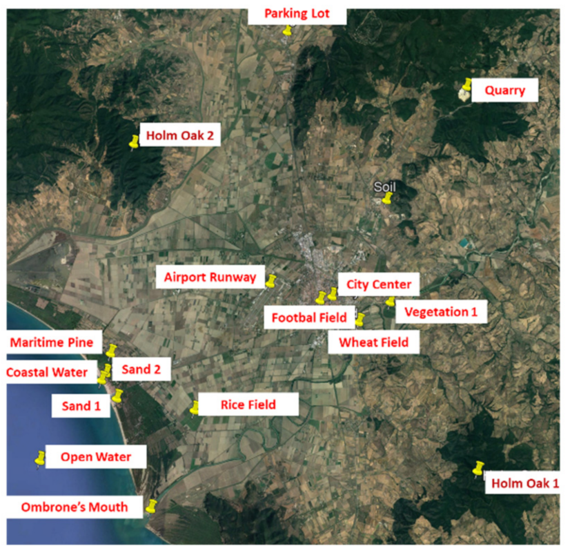
Our experiments focus on four images concerning the same scene and are collected at different times with different acquisition conditions. The scene includes several application scenarios such as urban, rural, and coastal regions and is a good test case for the proposed analysis. The scene has a spatial extent of and is centered near the city of Grosseto, in the south of Tuscany, Italy. In Figure 1 we show a high spatial resolution image of the region of interest taken by Google Earth. In the same image, we have marked the position of some “targets” that will be adopted to discuss the results. Selected targets include both natural surfaces and artificial surfaces.

Figure 1.
Image of the scene of interest taken by Google Earth. Landmarks indicate the position of the natural and artificial surfaces selected to discuss the results.
Table 3 shows, for each image, (a) the acquisition date, (b) the solar zenith angle , (c) the sensor viewing angle , (d) the relative azimuth angle between the incident solar direction and the direction of propagation of the scattered radiance , and (e) the cloud cover percentage. The angles reported in Table 3 are averaged over all the pixels of each image. Notice that the images named DAY2, DAY3, and DAY4 were collected approximately with the same solar zenith angle and sensor viewing angle and are relatively close in time. DAY1 data were acquired at a temporal distance greater than two months from the others and with a different acquisition geometry. As an example, Figure 2 shows the PRISMA true color (Red Green Blue: RGB) composite image taken on 8 July 2020 (DAY4).
Table 3.
Acquisition date and acquisition geometry parameters for the images chosen for the experiments.
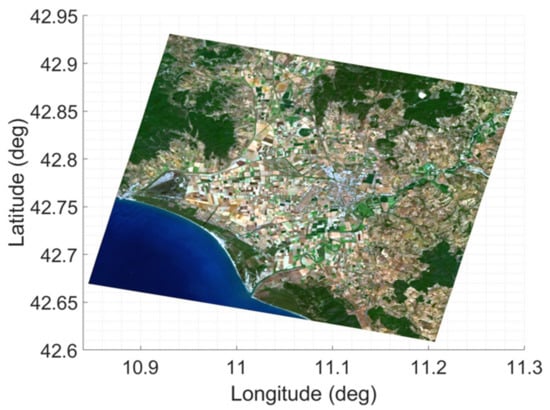
Figure 2.
PRISMA true color (Red Green Blue: RGB) composite image taken on 8 July 2020 (DAY4).
On the basis of the acquisition time of the images, in the learning phase of the LBAC algorithm and in the visibility estimation algorithm, we adopted the LUTs derived by considering the Mid-Latitude Summer Modtran model. Furthermore, on the basis of the characteristic of the scene, we have considered two distinct aerosol models (parameter IHAZE of Modtran): the rural aerosol model for land pixels and the maritime aerosol model for pixels of the Tyrrhenian Sea. The basis matrix of the reflectance subspace is obtained by the procedure in [20,35] assuming a rank of 40.
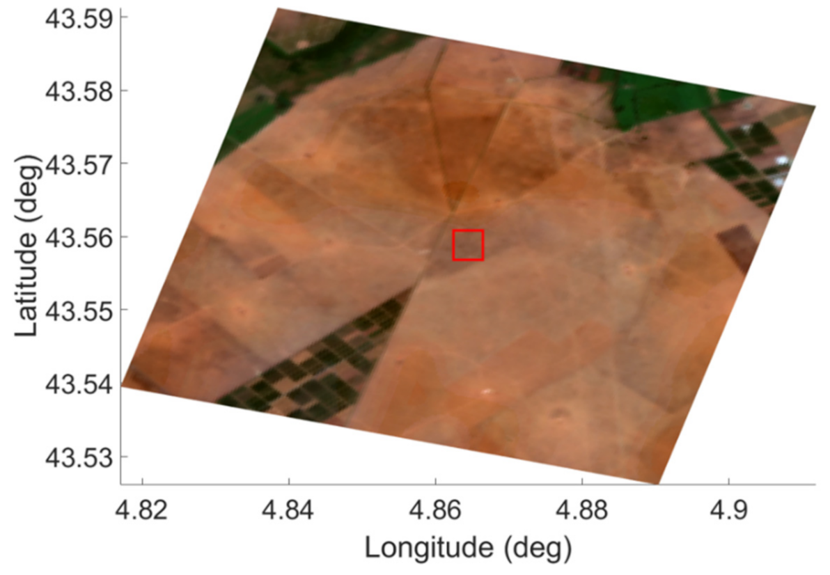
Before analyzing the results obtained on the above-mentioned images, we show the first example concerning a different image that is chosen because it is one of the rare cases in which in situ measurements are available. Specifically, we refer to the image acquired on 8 August 2020 (at 10:47) over the La Crau site in France, where one of the measurement stations of the RadCalNet network [36] operates. RadCalNet is an initiative of the Working Group on Calibration and Validation of the Committee on Earth Observation Satellites (CEOS), aimed at collecting in situ reflectance and atmospheric measurements to aid in the post-launch radiometric calibration and validation of optical imaging sensor data. La Crau station measures data representative of a very small area (compared to the PRISMA GSD) corresponding to a disk of 30 m radius on latitude 43.55885 degrees and longitude 4.864472 degrees covered by pebbly soil with sparse vegetation. In situ spectral reflectance measurements were performed by an ASD FieldSpec-4 spectroradiometer mounted on a tripod with a time interval of 30 min between 09:00 to 15:00 local standard time. The reflectance spectra and the measurement uncertainty in the spectral range from 400 nm to 2410 nm are made available. Note that the La Crau site was not specifically conceived for validation of PRISMA L2C data products and in general for L2 data from spaceborne sensors. To the best of our knowledge, a calibration/validation site specifically designed for PRISMA data is not yet available. Consequently, La Crau data cannot be used to assess the performance of an AC algorithm applied to PRISMA data, but can only be adopted to give an example of the goodness of the AC results.
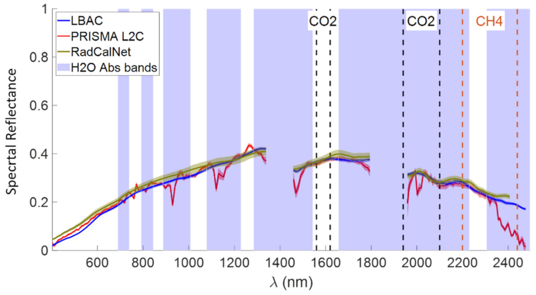
In Figure 3, we show the true color composite (RGB) representation of a portion of the PRISMA image collected on 8 August 2020 on the La Crau site; the red box indicates the region containing the measurement field. In Figure 4, the in situ reflectance spectra, measured at the same time of the PRISMA overpass, are compared in terms of error plot with the spectra provided by the LBAC and those included in the L2C PRISMA image. To consider the uncertainty about the pixel coordinates of the measurement field, we consider for both the LBAC results and the PRISMA L2C data an area of 5 × 5 pixels centered on the site coordinates. In the figure, the absorption bands due to CO2 are delimited by black dashed vertical lines, and the absorption spectral window due to CH4 is delimited by red dashed vertical lines. The blue transparent patches indicate the water absorption bands. Notice that for the spectra in Figure 4, and for all the spectra shown in the rest of the paper, we do not consider the reflectance values in the water absorption bands near 1370 nm and 1880 nm because all the solar radiation is absorbed by the water molecules in the atmosphere.
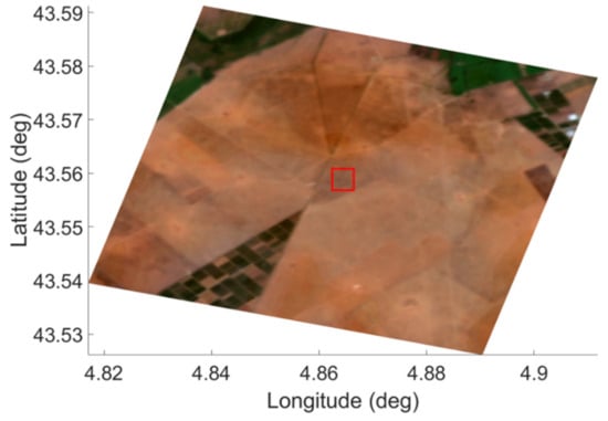
Figure 3.
RGB representation of a portion of the PRISMA image on the La Crau site. The red box indicates the area including the measurement field.
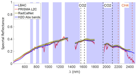
Figure 4.
Error plots of the spectral reflectance from RadCalNet, LBAC, and PRISMA L2C.
Results in Figure 4 show that both the LBAC and the AC PRISMA algorithm provide reflectance spectra very similar to the measured one with the mean relative errors in the order of 7% and 13%, respectively. The shape of the spectral reflectance obtained by both algorithms is very close to that measured on the ground. However, in this example, the LBAC outperforms the AC PRISMA algorithm. The LBAC reflectance closely follows the smooth behavior of the in situ reflectance, while the L2C PRISMA data exhibit artifacts (high-frequency variations) that are more evident in (a) the water absorption bands around 940 nm, 1130 nm, and above 2300 nm, and (b) in the CO2 absorption band around 2100 nm. The possible causes of those effects will be discussed in the next section.
4.2. Reflectance Analysis
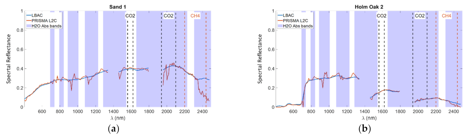
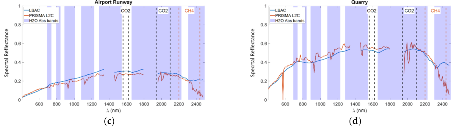
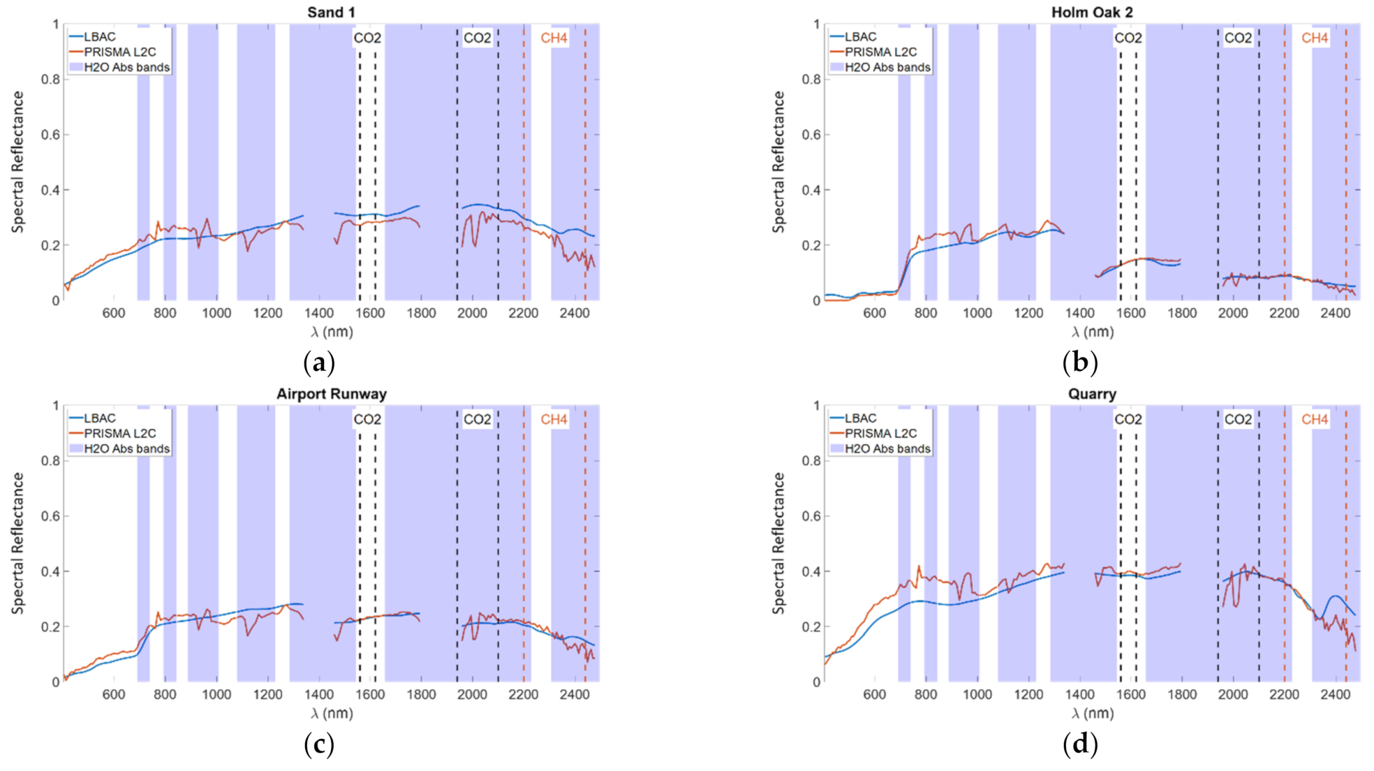
We start this sub-section by discussing the results concerning the DAY4 image and, specifically, four targets corresponding to both natural and artificial surfaces. As to the natural surfaces, we consider two pixels belonging to a beach (Sand 1) and to a holm oak forest (Holm Oak 2), respectively. The artificial surface pixels are selected from the airport runway (Airport Runway) and the rock quarry (Quarry), in the upper right part of the image. Figure 5a–d graphically compare, for each target, the spectral reflectance obtained by the LBAC (blue plot) with the L2C PRISMA product (red plot).
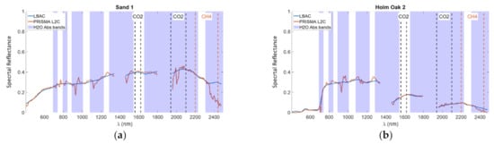
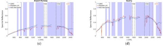
Figure 5.
DAY4. Graphical comparison of the spectral reflectance obtained by the LBAC and the PRISMA L2C product for the targets: (a) Sand 1, (b) Holm Oak 2, (c) Airport Runway, and (d) Quarry. The transparent blue patches indicate the water absorption bands. In the figures the CO2 and the CH4 absorption bands are also indicated.
Several conclusions can be drawn from the results in Figure 5a–d. We can see that the general behavior of the spectra derived by the two AC algorithms is quite similar, and, in both the cases, the main absorption effects due to water vapor, CO2 and CH4 are substantially compensated. The LBAC reflectance’s are smoother than those obtained by the AC PRISMA algorithm.
It is well-known that below 2500 nm, the spectral reflectance of most natural and man-made surfaces hardly ever shows narrow absorption bands even at the high spectral resolutions characterizing hyperspectral sensors. Specifically, several studies and experimental measurements [16,21] show that the spectral rate of change of the reflectance is much slower than that of the corresponding radiance. PB algorithms often provide atmospherically compensated data characterized by spectral artifacts, especially in the strongest absorption bands. These artifacts are generally due to different causes [16], such as systematic errors in the atmospheric absorption model, uncertainties in the solar reference spectrum, spectral residual calibration errors, and non-perfect radiometric calibration of the radiance data. In addition, non-systematic errors are induced by random variations due to photon noise and readout noise in the detector electronics. The presence of those artifacts motivates the practice of applying spectral polishing algorithms to the retrieved reflectance spectra in order to smooth them [21,33].
With reference to the experiment under consideration, we can observe that the AC PRISMA algorithm, which does not include (to the best of our knowledge) a spectral polishing procedure, seems to be not immune to the above-mentioned problems. The provided reflectance spectra exhibit systematic artifacts that suggest the possible presence of small errors in the calibration process or in the atmospheric model. We specifically refer to the sharp variations in the two water absorption bands around 940 nm and 1130 nm, and in the CO2 absorption band around 2100 nm.
Conversely, the LBAC results do not exhibit such kinds of artifacts and show better robustness to potential systematic and non-systematic spectral artifacts. This result is intrinsically related to the adopted learning strategy which relies on a database containing the measured reflectance spectrum of more than 3000 man-made materials, vegetation, water, soils, and minerals. The spectra in the database are smooth and do not have high-frequency variations in the spectral domain. Furthermore, enclosing the main sources of noise occurring in the hyperspectral data in the learning mechanism, makes the LBAC robust to incorrect calibration errors and random noise. The specific learning strategy behind the LBAC gives the algorithm an inherent polishing ability which is quite useful in many application fields such as land use/land cover, water quality, hydrology studies of snow and ice, basic mineralogical analyses, and some terrestrial and aquatic ecosystem investigations. Thus, in most applications, it is certainly a strength of LBAC and makes it a very promising approach, especially to process the low signal-to-noise ratio data and non-perfectly calibrated images. However, that intrinsic polishing effect could be a limit of LBAC in those applications where one is interested in searching materials whose reflectance is characterized by narrow-band spectral features or, in general, not well represented as a linear combination of the spectra in the database . This is, for example, the case of specific gas plumes, canopy chemistry, or environmental contaminants. In those cases, LBAC, in its current form, may not preserve the relevant spectral features. In general, when the reflectance of a given material is not well represented as a combination of the spectra in , one may lose the features that allow the discrimination of that material. This can occur also in the case of man-made target detection applications, when the signature of the target of interest could have an “anomalous” spectral behavior, in the sense that it cannot be obtained as a linear combination of the spectra in .
However, the approach in [20] is quite general and several modifications within the learning-based framework can be made to extend the capabilities of the resulting algorithm. For instance, regression functions more complicated than linear ones (e.g., deep neural networks) can be adopted to explore non-linear structures in the data. Another possible modification may concern the database adopted in the learning phase and for the representation of the reflectance subspace. For example, the database could be application-driven and populated with data including the spectral features that are significant for the application of interest. Possible solutions to the drawbacks of the LBAC version considered in this paper are under investigation and they are the focus of our ongoing activity.
To provide evidence of the effectiveness of the proposed approach in the analyzed image (DAY4), we have computed the Squared Error (SE) between the reflectance of each pixel estimated by the LBAC and that given by the AC PRISMA algorithm:
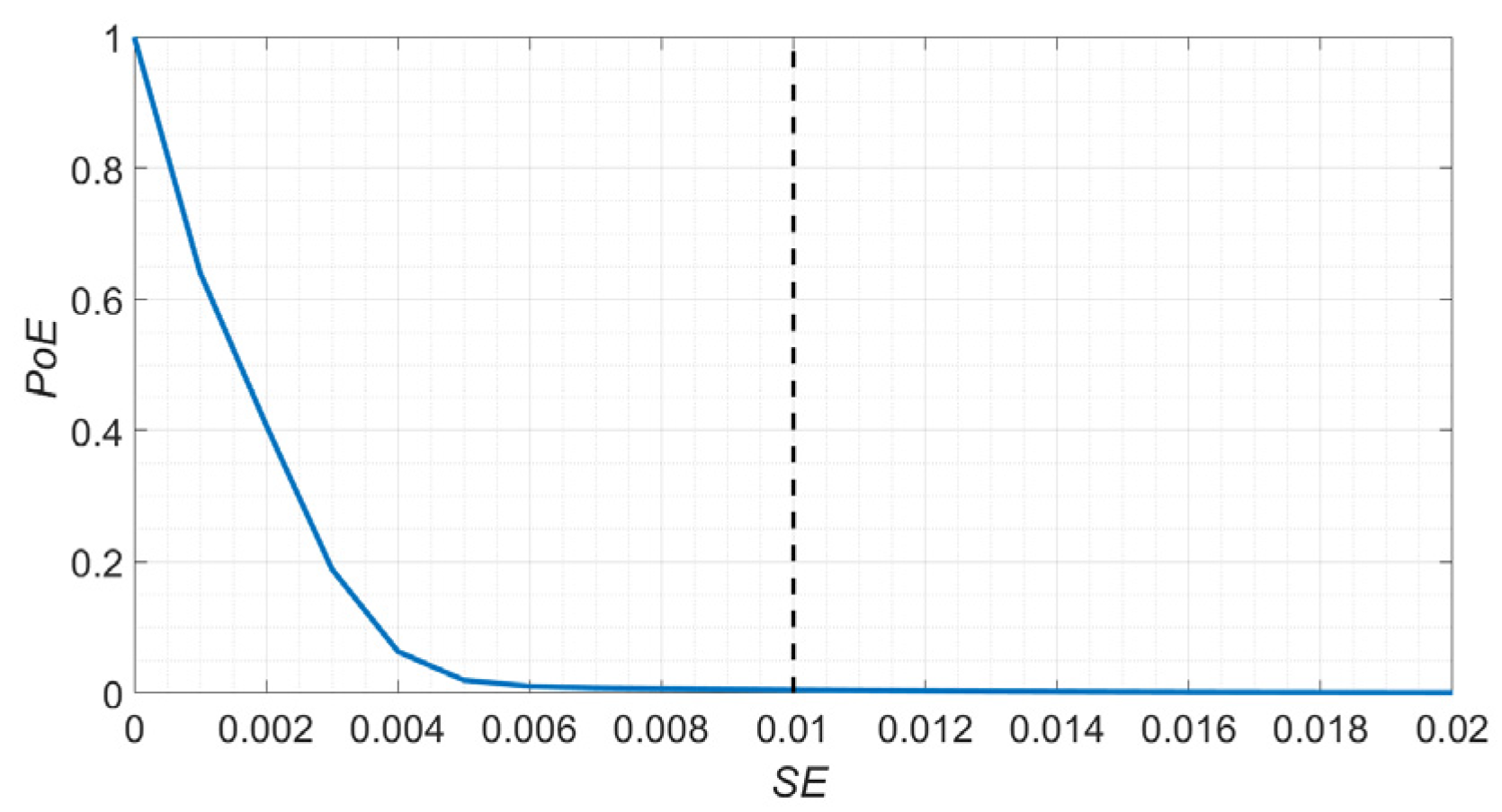
In Equation (6), and are the coordinates of the image pixel, is the number of spectral bands, is the reflectance estimated by LBAC in the pixel and is the reflectance provided by the AC PRISMA algorithm on the same pixel. The Mean SE (MSE) obtained by averaging the SE on the whole DAY4 image is very low and equal to . In order to provide information about the spread of the distribution of , we consider its Probability of Exceedance () defined as the complement of the cumulative distribution function () estimated on the whole image, i.e., . of for DAY4 image (Figure 6) shows that most of the image pixels have lower than , and the percentage of image pixels with greater than is lower than 0.47% ().
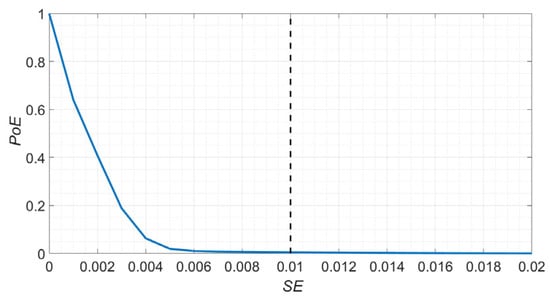
Figure 6.
Value of the PoE of SE for the DAY 4 image.
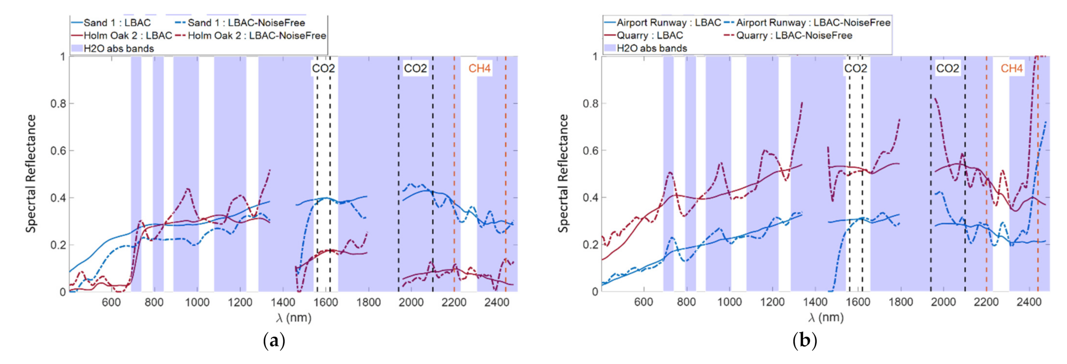
As to the benefits linked to the inclusion of the noise sources in the learning strategy, it was deeply investigated on simulated data in [20], by analyzing the results obtained by the version of the LBAC trained without taking into account noise. Results in Figure 7a,b provide further evidence. In those figures, we compare the reflectance spectra obtained by applying both the LBAC and its version trained without considering noise (LBAC-NoiseFree). The poor performance of the LBAC–NoiseFree is clear proof of the importance of introducing noise in the learning phase.
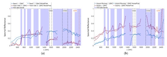
Figure 7.
DAY4. Comparison of the results provided by LBAC and LBAC-NoiseFree on the targets: (a) Sand 1, Holm Oak 2, and (b) Airport Runway, Quarry.
Another conclusion is that, opposite to traditional PB methods, the LBAC is insensitive to bad pixels occurring in the image. This is evident in Figure 5b,d. Specifically, the sharp and narrow transitions to zero in the PRISMA L2C spectrum of Holm Oak 2 around 700 nm and Quarry at 570 nm are caused by bad pixels that are properly flagged in the PRISMA data products. Notice that the LBAC automatically reconstructs the observed spectra in those bad bands without exploiting the information about their location in the image.
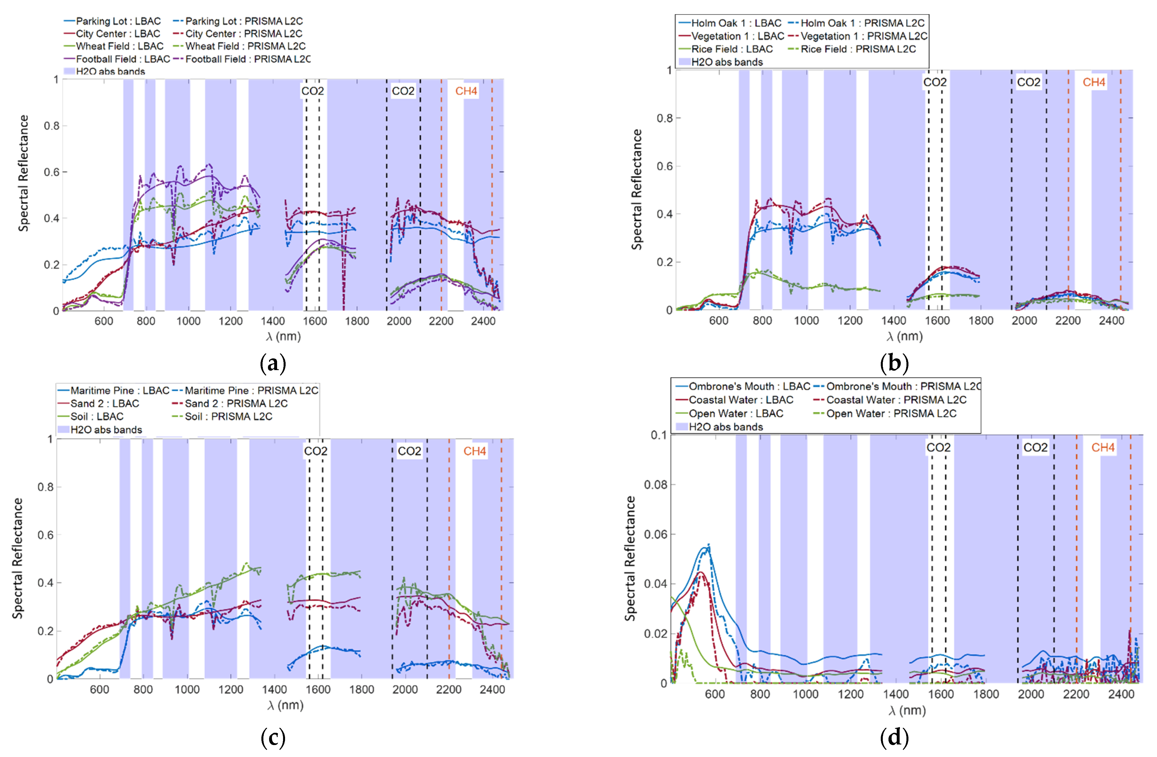
For completeness, in Figure 8 we summarize the results obtained on all the targets considered in this experiment. Results in Figure 8 confirm all the previous conclusions.
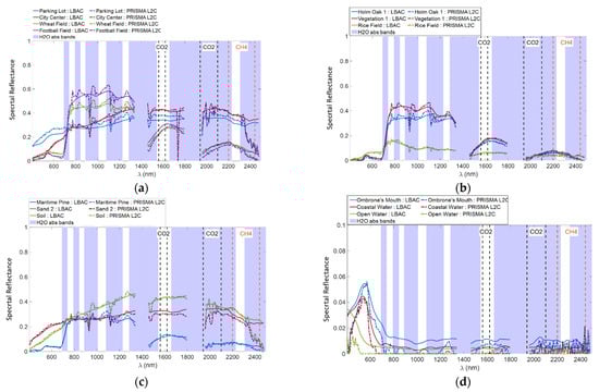
Figure 8.
DAY4. Graphical comparison of the spectral reflectance obtained by the LBAC and the PRISMA L2C product for the targets: (a) Parking Lot, City Center, Wheat Field and Football Field; (b) Holm Oak 1, Vegetation 1, and Rice Field; (c) Maritime Pine, Sand2, and Soil, (d) Ombrone’s Mouth, Coastal Water, and Open Water. The transparent blue patches indicate the water absorption bands. In the figures, the CO2 and the CH4 absorption bands are also indicated.
An analysis similar to that described in the previous part of this section has been carried out on the DAY1 image that was acquired under different atmospheric and viewing conditions. A synthesis of the results obtained is reported in the following. Specifically, in Figure 9 we compare the spectra derived by the LBAC with those provided by the PRISMA L2C product for the same targets considered in the previous experiment: Holm Oak 2, Sand 1, Airport Runway, and Quarry. We note that the spectra derived by the LBAC and by the AC PRISMA algorithm follow the same general trend and that in both cases the main absorption effects are compensated. However, we note a slight difference in the derived spectra in the channels corresponding to wavelengths falling in the visible spectral range between 600 nm and 900 nm. In absence of ground truth data, we cannot determine which of the two results is more correct. We can only make hypotheses about the causes of that misalignment. For instance, it could be determined (1) by a difference in the derivation of the LUTs adopted by the two algorithms, (2) by the fact that the LBAC, in its current version, does not account for the terrain elevation, (3) errors in the visibility estimation. However, the MSE obtained all over the image is and the analysis of the shows that the percentage of image pixels with greater than is lower than 0.092% ().
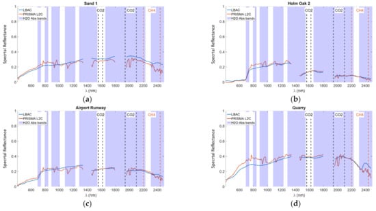
Figure 9.
DAY1. Graphical comparison between the spectral reflectance obtained by the LBAC and the PRISMA L2C product for the targets: (a) Sand 1, (b) Holm Oak 2, (c) Airport Runway, (d) Quarry. The transparent blue patches indicate the water absorption bands. In the figures, the CO2 and the CH4 absorption bands are also indicated.
As in the previous experiment, we note that PRISMA L2C data exhibit possible artifacts in the water absorption bands around 940 nm and 1130 nm and in the CO2 absorption band around 2100 nm. Such artifacts seem systematic and support the thesis of potential residual errors in the radiometric calibration of the data in the absorption bands or errors in the model of the atmospheric radiometric quantities. The non-systematic variations can be generated by random noise affecting the measurements. LBAC, providing smoother spectra, confirms its robustness to both residual calibration errors and random noise. The above considerations can be extended to all the targets analyzed in our experiments whose results are not reported here for brevity.
It is worth noting that, in all the results shown (included those of the La Crau site), there is a difference between the spectra provided by the LBAC and those of the PRISMA L2C product in the 2400 nm water absorption band. The difference could be due to an imperfect compensation, in the PRISMA L2C product, of the strong water absorption effect. This possible interpretation is motivated in the following. As is shown in the next part of this section, the DAY1 image was characterized by values (close to 0.5 ) lower than those of the DAY4 image (close to 2 ). Consequently, potential errors in the compensation of water absorption are supposed to have a lower impact on the results of the DAY1 image. Indeed, comparing Figure 5 with Figure 9, we note that the difference between the LBAC spectra and the PRISMA L2C data in the DAY1 image (Figure 9) is strongly reduced with respect to that observed in the results concerning the DAY4 image (Figure 5).
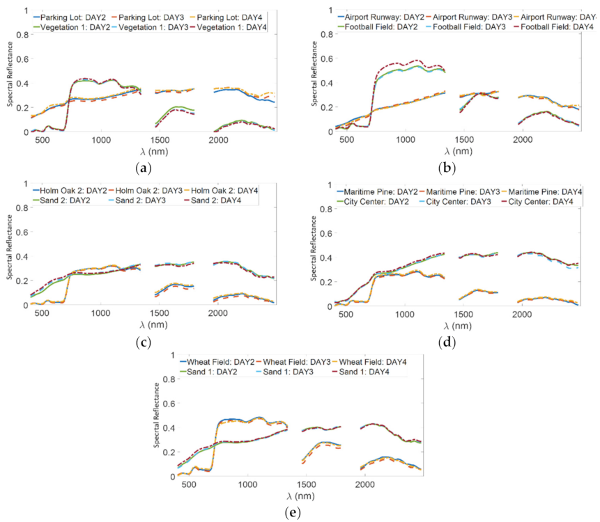
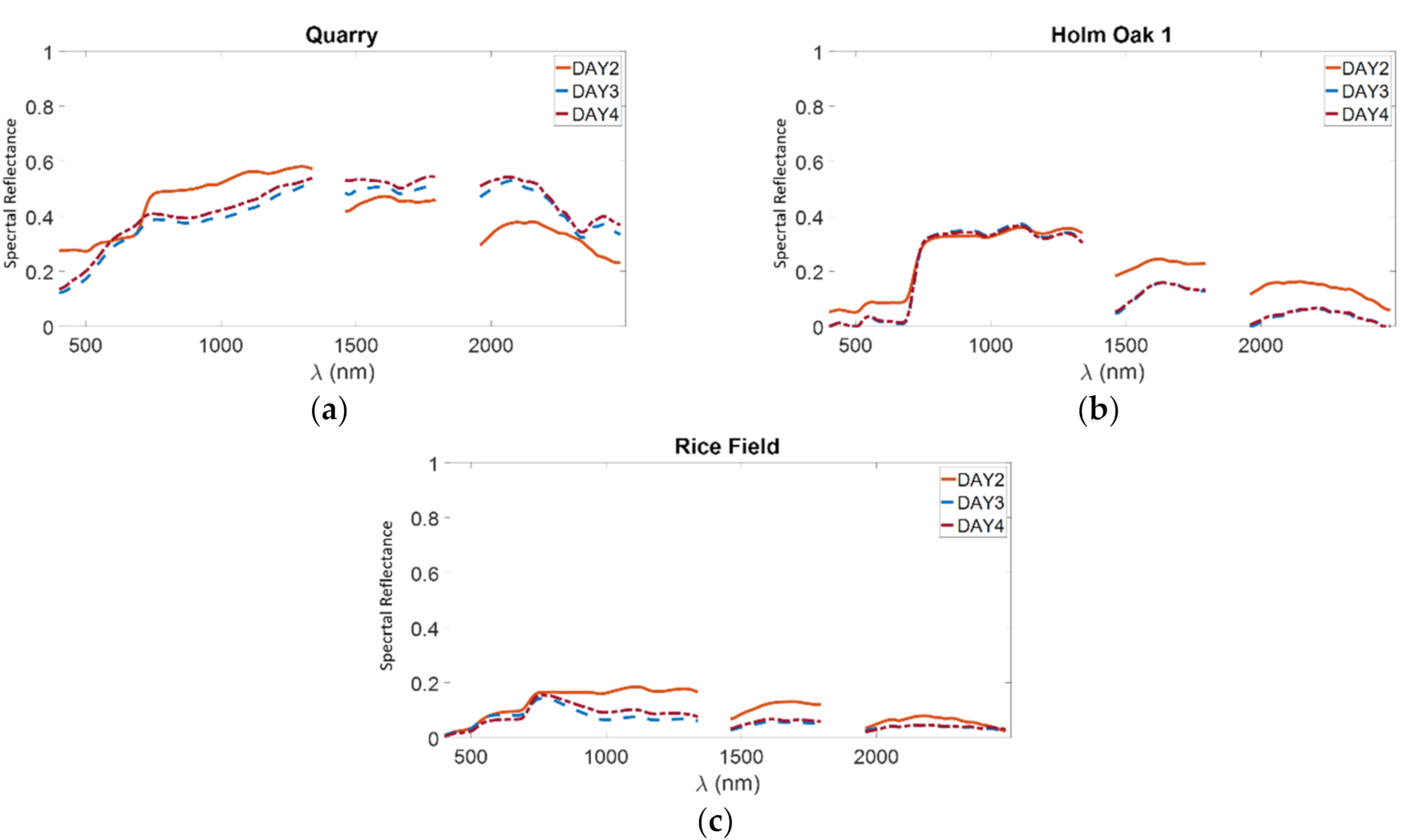
Another noteworthy result regards the three images named DAY2, DAY3, and DAY4. These images were collected approximately in the same period of the year and practically with the same incidence and observation angles. Therefore, the effects of seasonal changes and those of the anisotropic response of the observed surfaces to the incident radiation are expected to be negligible. This means that, if the AC algorithm works well, the reflectance spectra derived for the same surface in the scene in the three images must be very similar. The previous claim is verified by the results obtained by the LBAC on the three images. Specifically, Figure 10 and Figure 11 show the reflectance spectra derived by the LBAC on the three images for all the in-land targets considered in our experiments. Notice that the spectra are practically the same for almost all the targets. The only exception is represented by the targets Quarry, Holm Oak 1, and Rice Field in the DAY2 image (Figure 11). In the case of Holm Oak 1 and Quarry, the difference in the spectra is certainly due to the fact that both the targets were covered by cloud in the DAY 2 image. For the Rice Field target, the variation in the spectra could be due to the greater presence of water in the field at the time of the acquisition of the DAY3 and DAY4 images. Of course, the above discussion also applies to the spectra of the PRISMA L2C data in the three images.
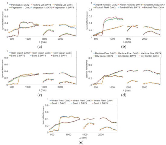
Figure 10.
Comparison of the spectra derived by the LBAC on the considered targets in the three images named DAY2, DAY3, and DAY4 (a–e).
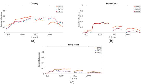
Figure 11.
Comparison of the spectra derived by the LBAC on the targets Quarry (a), Holm Oak 1 (b), and Rice Field (c) in the three images named DAY2, DAY3, and DAY4.
4.3. LBAC Based CWV Retrieval: Results
In this sub-section, we present the results obtained by applying the retrieval algorithm described in Section 3 and based on the LBAC. Such results are compared with the estimates included in the PRISMA L2C product and with those obtained by applying the well-known Atmospherically Pre-corrected Differential Absorption (APDA) technique proposed in [29] that is adopted by several PB atmospheric compensation algorithms. APDA was applied to the water absorption spectral window around 940 nm.
Figure 12 shows, in the form of error bars, the mean values and the standard deviations of the estimates obtained by the means of the LBAC-based procedure, those included in the PRISMA L2C product, and those obtained by APDA. We excluded the estimates from water pixels where the three procedures do not provide reliable results because of the low signal-to-noise ratio in the water absorption bands. In all the considered cases, the proposed algorithm provides values quite close to those included in the PRISMA L2C product and those derived by APDA. Specifically, the LBAC-based procedure attains values of very similar to those provided by APDA. Both the algorithms give estimated values greater than (approximately 20%) those provided by the PRISMA AC algorithm. However, the estimates from the three algorithms are highly correlated. The correlation coefficients between the LBAC and the PRISMA L2C are 0.72 for DAY1, 0.93 for DAY2, 0.89 for DAY3, and 0.91 for DAY4. Those between the LBAC and APDA are 0.73 for DAY1, 0.93 for DAY2, 0.9 for DAY3, and 0.92 for DAY4. The APDA and PRISMA L2C products, both exploiting the differential absorption approach, have correlation coefficients greater than 0.95 in all the considered images. For completeness, in Figure 13 we show the (estimated) probability density functions (pdf) for the values obtained by the three algorithms on the four images. For each image, the pdf of the estimates obtained by the proposed procedure and by the PRISMA L2C product have approximately the same shape, but they seem to differ for a shift. This is especially true for the DAY2, DAY3, and DAY4 images. As for the comparison between the LBAC-based procedure and the APDA, we note that the pdfs are very close in shape and position.
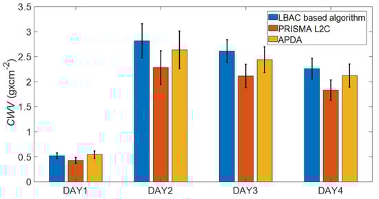
Figure 12.
Mean values and standard deviations of CWV estimates from the LBAC-based algorithm and the PRISMA L2C product.
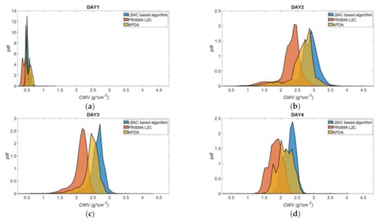
Figure 13.
Estimated probability density function (pdf) of the CWV values provided by the LBAC-based procedure and the PRISMA L2C product on: (a) DAY1 image, (b) DAY2 image, (c) DAY3 image, and (d) DAY4 image.
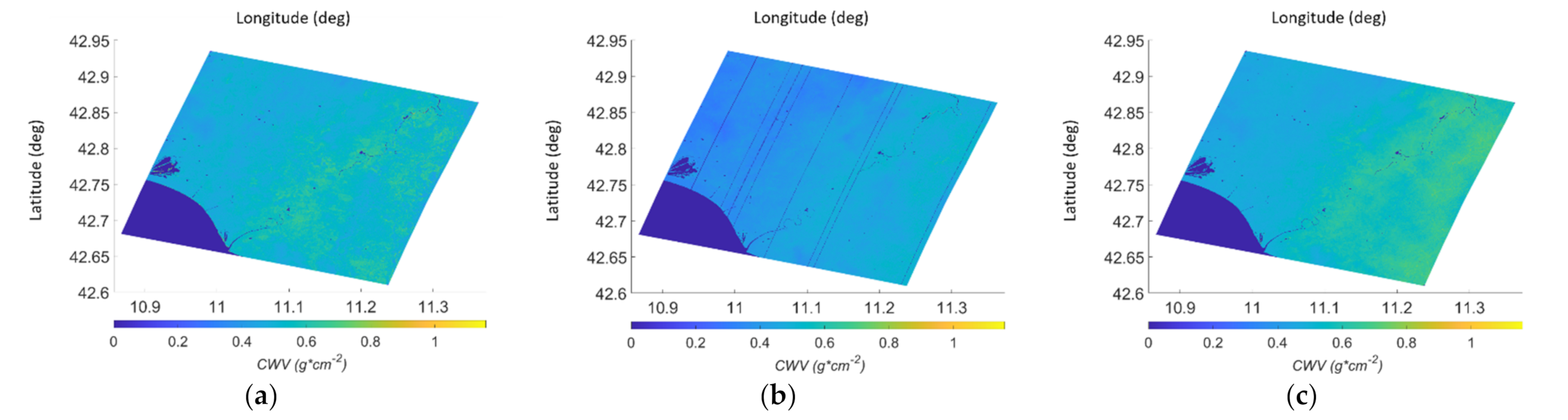
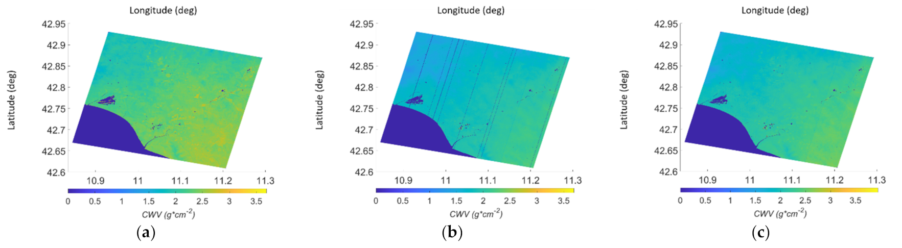
As an example, in Figure 14 and Figure 15 we show the maps for the DAY1 image (Figure 14) and the DAY4 image (Figure 15) obtained by the proposed technique, those included in the PRISMA L2C data and those obtained by the APDA algorithm. In all the maps, the water pixels are masked. Notice that the stripes in the cross-track direction appearing in the map included in the PRISMA L2C product (Figure 14b and Figure 15b) correspond to bad pixels that are properly indicated in the provided product.
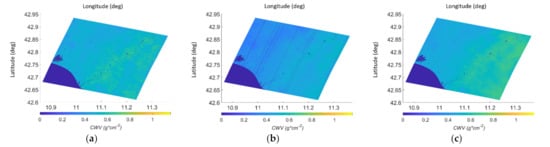
Figure 14.
DAY1: (a) CWV map obtained by the proposed procedure; (b) CWV map from the PRISMA L2C product; (c) CWV map obtained by the APDA algorithm.

Figure 15.
DAY4: (a) CWV map obtained by the proposed procedure; (b) CWV map from the PRISMA L2C product; (c) CWV map obtained by the APDA algorithm.
5. Conclusions
The intent of this paper is to present an extension of the recently proposed LBAC algorithm to data acquired by a satellite hyperspectral sensor operating in the VNIR and SWIR spectral intervals, along with a discussion of the results obtained on the first available data of the hyperspectral EO mission PRISMA. After a brief summary of the algorithm, we have emphasized the modifications made for its extension to satellite data and to the SWIR spectral domain. Furthermore, we have introduced a curve fitting-based retrieval procedure that exploits the reflectance estimates provided by LBAC.
Results on four different PRISMA images of the same scene have been presented and discussed. As a consequence of the lack of reference data and ground truth information, a qualitative analysis has been performed by comparing the results provided by the learning-based approach with those distributed by ASI as part of the PRISMA products. The analysis confirmed most of the conclusions drawn from the application of the LBAC to VNIR airborne hyperspectral data and showed that the LBAC can be effectively applied also to process VNIR-SWIR satellite data. In particular, the smooth behavior of the LBAC-retrieved spectra confirmed the robustness of the algorithm to random noise and residual radiometric and spectral calibration errors. Results of the retrieval algorithm are quite correlated to those included in the PRISMA L2C product. However, we observed a systematic difference between the values provided by the LBAC-based estimation algorithm and the PRISMA L2C products. In the absence of ground truth data, it is not possible to draw quantitative conclusions on the performance of the two algorithms.
In light of the results of the LBAC on the VNIR airborne data [20] and on the VNIR-SWIR satellite data, we can state that it is a promising unconventional approach to atmospheric compensation especially when perfect radiometric/spectral calibration cannot be obtained. LBAC adds to the plethora of existing AC methods with its strengths and weaknesses. As claimed by several authors, an AC algorithm that works the best in all conditions does not exist and the availability of alternative methods enriches the opportunity of choosing the most suitable solution for the case of interest.
The promising results of LBAC encourage further efforts to improve its performance and to extend its capabilities by including (a) terrain elevation, (b) anisotropic response of the surface to the incident radiation, and (c) more complicated aerosol profiles. Surely, one of the issues that needs to be further investigated is related to the estimation of the visibility. In the current version of the algorithm, it is obtained by a dark pixel-based approach. It is in general effective in regions containing a surface with very low spectral reflectance in specific spectral bands, but it tends to underestimate the visibility in the absence of dark pixels. We are studying new visibility estimation strategies that involve and exploit information provided by other satellite missions that supply global aerosol optical thickness products validated by means of in situ measurements. For instance, we would like to exploit data from the Moderate Resolution Imaging Spectroradiometer (MODIS) aboard NASA’s Aqua and Terra satellites, and the Visible Infrared Imaging Radiometer Suite (VIIRS) aboard the joint NASA/NOAA Suomi National Polar-orbiting Partnership (Suomi NPP) and NOAA-20 satellites.
It is worth noting that the LBAC provides good results on spectra having a smooth behavior, as in the case of most natural and man-made materials, but it might be less accurate in estimating the reflectance of materials featuring narrow spectral features, such as gases or minerals, or, in general, for those materials whose spectral behavior cannot be obtained as a linear combination of the spectra included in the adopted database. Possible solutions to this problem include the use of more complete databases that could be enriched or modified by a priori knowledge in order to match the specific characteristics of the scene under analysis. For instance, an “application-driven” spectral library might be used, populated, or enriched with specific spectra of interest in the considered application scenario. The analysis of such kinds of solutions is the subject of our ongoing activities.
Author Contributions
Conceptualization, N.A. and M.D.; methodology, N.A.; software, N.A. and G.P.; validation, N.A.; formal analysis, N.A.; investigation, N.A. and G.P.; resources, G.C.; data curation, N.A. and G.C.; writing—original draft preparation, N.A.; writing—review and editing, N.A.; supervision, M.D., G.P. and G.C.; project administration, G.C. All authors have read and agreed to the published version of the manuscript.
Funding
This research received no external funding.
Institutional Review Board Statement
Not applicable.
Informed Consent Statement
Not applicable.
Data Availability Statement
Not applicable.
Acknowledgments
This project was carried out using PRISMA products, © of the Italian Space Agency (ASI), delivered under an ASI License to use.
Conflicts of Interest
The authors declare no conflict of interest.
References
- Chang, C.-I. (Ed.) Hyperspectral Data Exploitation: Theory and Applications; John Wiley & Sons: Hoboken, NJ, USA, 2007. [Google Scholar]
- Transon, J.; d’Andrimont, R.; Maugnard, A.; Defourny, P. Survey of Hyperspectral Earth Observation Applications from Space in the Sentinel-2 Context. Remote Sens. 2018, 10, 157. [Google Scholar] [CrossRef] [Green Version]
- van der Meer, F.D.; van der Werff, H.M.A.; van Ruitenbeek, F.J.A.; Hecker, C.A.; Bakker, W.H.; Noomen, M.F.; van der Meijde, M.; Carranza, E.J.M.; de Smeth, J.B.; Woldai, T. Multi- and Hyperspectral Geologic Remote Sensing: A Review. Int. J. Appl. Earth Obs. Geoinform. 2012, 14, 112–128. [Google Scholar] [CrossRef]
- Thenkabail, P.S.; Gumma, M.K.; Teluguntla, P.; Mohammed, I.A. Hyperspectral remote sensing of vegetation and agricultural crops. Photogramm. Eng. Remote Sens. 2014, 80, 697–709. [Google Scholar]
- Adam, E.; Mutanga, E.O.; Rugege, D. Multispectral and Hyperspectral Remote Sensing for Identification and Mapping of Wetland Vegetation: A Review. Wetl. Ecol. Manag. 2010, 18, 281–296. [Google Scholar] [CrossRef]
- Dekker, A.; Brando, V.; Anstee, J.; Pinnel, N.; Held, A. Preliminary assessment of the performance of Hyperion in coastal waters. Cal/Val activities in Moreton Bay, Queensland, Australia. In Proceedings of the IEEE 2001 International Geoscience and Remote Sensing Symposium (IGARSS), Sydney, Australia, 9–13 July 2001; Volume 6, pp. 2665–2667. [Google Scholar]
- Pignatti, S.; Acito, N.; Amato, U.; Casa, R.; de Bonis, R.; Diani, M.; Laneve, G.; Matteoli, S.; Palombo, A.; Pascucci, S.; et al. Development of algorithms and products for supporting the Italian hyperspectral PRISMA mission: The SAP4PRISMA project. In Proceedings of the IEEE International Geoscience and Remote Sensing Symposium, IGARSS ’12, Munich, Germany, 22–27 July 2012; pp. 127–130. [Google Scholar]
- Pignatti, S.; Palombo, A.; Pascucci, S.; Romano, F.; Santini, F.; Simoniello, T.; Amato, U.; Cuomo, V.; Acito, N.; Diani, M.; et al. The PRISMA hyperspectral mission: Science activities and opportunities for agriculture and land monitoring. In Proceedings of the IEEE International Geoscience and Remote Sensing Symposium, IGARSS ’13, Melbourne, VIC, Australia, 21–26 July 2013; pp. 4558–4661. [Google Scholar]
- Guarini, R.; Loizzo, R.; Facchinetti, C.; Longo, F.; Ponticelli, B.; Faraci, M.; Dami, M.; Cosi, M.; Amoruso, L.; de Pasquale, V.; et al. Prisma Hyperspectral Mission Products. In Proceedings of the IEEE International Geoscience and Remote Sensing Symposium, IGARSS ’18, Valencia, Spain, 22–27 July 2018; pp. 179–182. [Google Scholar]
- Loizzo, R.; Daraio, M.; Guarini, R.; Longo, F.; Lorusso, R.; Dini, L.; Lopinto, E. Prisma Mission Status and Perspective. In Proceedings of the IEEE International Geoscience and Remote Sensing Symposium, IGARSS ’19, Yokohama, Japan, 28 July–2 August 2019; pp. 4503–4506. [Google Scholar]
- Available online: http://prisma-i.it/index.php/en/ (accessed on 16 July 2020).
- Schott, J.R. Remote Sensing: The Image Chain Approach, 2nd ed.; Oxford University Press: New York, NY, USA, 2007. [Google Scholar]
- Acito, N.; Diani, M. Unsupervised Atmospheric Compensation of airborne hyperspectral images in the VNIR spectral range. IEEE Trans. Geosci. Remote Sens. 2018, 56, 3924–3940. [Google Scholar] [CrossRef]
- Ientilucci, E.J.; Adler-Golden, S. Atmospheric compensation of hyperspectral data: An overview and review of In-Scene and Physics-Based approaches. IEEE Geosci. Remote Sens. Mag. 2019, 7, 31–50. [Google Scholar] [CrossRef]
- Acito, N.; Diani, M. Atmospheric Column Water Vapor Retrieval from Hyperspectral VNIR Data Based on Low-Rank Subspace Projection. IEEE Trans. Geosci. Remote Sens. 2018, 56, 3924–3940. [Google Scholar] [CrossRef]
- Thompson, D.R.; Guanter, L.; Berk, A.; Gao, B.-C.; Richter, R.; Schläpfer, D.; Thome, K.J. Retrieval of Atmospheric Parameters and Surface Reflectance form Visible and Shortwave Infrared Imaging Spectroscopy Data. Surv. Geophys. 2019, 40, 333–360. [Google Scholar] [CrossRef] [Green Version]
- Kruse, F.A. Comparison of ATREM, ACORN, and FLAASH atmospheric corrections using low-altitude AVIRIS data of Boulder, CO. In Summaries of 13th JPL Airborne Geoscience Workshop; Jet Propulsion Lab.: Pasadena, CA, USA, 2004. [Google Scholar]
- Richter, R.; Schlaepfer, D. Geo-atmospheric processing of airborne imaging spectrometry data. Part 2: Atmospheric/topographic correction. Int. J. Remote Sens. 2002, 23, 2631–2649. [Google Scholar] [CrossRef]
- Berk, A.; Bernstein, L.S.; Robertson, D.C. MODTRAN: A Moderate Resolution Model for LOWTRAN 7. In Spectral Sciences; GLTR890122; National Technical Reports Library: Burlington, MA, USA, 1989. [Google Scholar]
- Acito, N.; Diani, M.; Corsini, G. Learning-based approach for atmospheric compensation of VNIR hyperspectral data. IEEE Trans. Geosci. Remote Sens. 2021, 59, 4218–4232. [Google Scholar] [CrossRef]
- Schläpfer, D.; Richter, R. Spectral polishing of high resolution imaging spectroscopy data. In Proceedings of the 7th SIG-IS workshop on imaging spectroscopy, Edinburgh, UK; 2011; p. 7. Available online: http://daniel-schlaepfer.ch/pdf/Schlaepfer_IS2011_polish.pdf (accessed on 27 July 2021).
- Baldridge, A.M.; Hook, S.J.; Grove, C.I.; Rivera, G. The ASTER Spectral Library Version 2.0. Remote Sens. Environ. 2009, 113, 711–715. [Google Scholar] [CrossRef]
- Clark, R.N.; Swayze, G.A.; Wise, R.A.; Live, K.E.; Hoefen, T.M.; Kokaly, R.F.; Sutley, S.J. USGS Digital Spectral Library splib06a: U.S. Geol. Surv. Data Ser. 2007, 231. [Google Scholar]
- Available online: http://opticleaf.ipgp.fr/index.php?page (accessed on 27 July 2021).
- Reinersman, P.N.; Carder, K.L. Monte Carlo simulation of the atmospheric point-spread function with application to correction for adjacency effect. Appl. Opt. 1995, 34, 4453–4471. [Google Scholar] [CrossRef] [PubMed]
- Skauli, T. Sensor noise informed representation of hyperspectral data, with benefits for image storage and processing. Opt. Express 2011, 19, 13031–13046. [Google Scholar] [CrossRef] [PubMed]
- Acito, N.; Diani, M.; Corsini, G. Signal-Dependent Noise Modeling and Model Parameter Estimation in Hyperspectral Images. IEEE Trans. Geos. Remote Sens. 2011, 49, 2957–2971. [Google Scholar] [CrossRef]
- Richter, R.; Schlaepfer, D.; Muller, A. An automatic atmospheric correction algorithm for visible/NIR imagery. Int. J. Remote Sens. 2006, 27, 2077–2085. [Google Scholar] [CrossRef]
- Available online: http://prisma.asi.it/missionselect/docs/PRISMA%20Product%20Specifications_Is2_3.pdf (accessed on 9 April 2021).
- Available online: https://sentinel.esa.int/web/sentinel/missions/sentinel-3 (accessed on 7 January 2021).
- Available online: https://ladsweb.modaps.eosdis.nasa.gov/missions-and-measurements/science-domain/aerosol (accessed on 7 January 2021).
- Sherwood, S.C.; Roca, R.; Weckwerth, T.M.; Andronova, N.G. Tropospheric water vapor, convection and Climate. Rev. Geophys. 2010, 48, 1–29. [Google Scholar] [CrossRef] [Green Version]
- Gao, B.C.; Goetz, A.F.H. Column atmospheric water vapor and vegetation liquid water retrievals from airborne imaging spectrometer data. J. Geophys. Res. Atmos. 1990, 95, 3549–3564. [Google Scholar] [CrossRef]
- Schlaepfer, D.; Borel, C.C.; Keller, J.; Itten, K.I. Atmospheric Precorrected Differential Absorption Technique to Retrieve Columnar Water Vapor. Remote Sens. Environ. 1998, 65, 353–366. [Google Scholar] [CrossRef]
- Gao, B.C.; Liu, M. A fast smoothing algorithm for post-processing of surface reflectance spectra retrieved from airborne imaging spectrometer data. Sensor 2013, 13, 13879–13891. [Google Scholar] [CrossRef] [PubMed]
- Available online: https://www.radcalnet.org/ (accessed on 16 April 2021).


Publisher’s Note: MDPI stays neutral with regard to jurisdictional claims in published maps and institutional affiliations. |
© 2021 by the authors. Licensee MDPI, Basel, Switzerland. This article is an open access article distributed under the terms and conditions of the Creative Commons Attribution (CC BY) license (https://creativecommons.org/licenses/by/4.0/).