Abstract
Ground-based multichannel microwave radiometers (GMRs) can observe the atmospheric microwave radiation brightness temperature at K-bands and V-bands and provide atmospheric temperature and humidity profiles with a relatively high temporal resolution. Currently, microwave radiometers are operated in many countries to observe the atmospheric temperature and humidity profiles. However, a theoretical analysis showed that a radiometer can be used to observe solar radiation. In this work, we improved the control algorithm and software of the antenna servo control system of the GMR so that it could track and observe the sun and we use this upgraded GMR to observe solar microwave radiation. During the observation, the GMR accurately tracked the sun and responded to the variation in solar radiation. Furthermore, we studied the feasibility for application of the GMR to measure the absolute brightness temperature (TB) of the sun. The results from the solar observation data at 22.235, 26.235, and 30.000 GHz showed that the GMR could accurately measure the TB of the sun. The derived solar TB measurements were 9950 ± 334, 10,351 ± 370, and 9217 ± 375 K at three frequencies. In a comparison with previous studies, we obtained average percentage deviations of 9.1%, 5.3%, and 4.5% at 22.235, 26.235, and 30.0 GHz, respectively. The results demonstrated that the TB of the sun retrieved from the GMR agreed well with the previous results in the literature. In addition, we also found that the GMR responded to the variation in sunspots and a positive relationship existed between the solar TB and the sunspot number. According to these results, it was demonstrated that the solar observation technique can broaden the field usage of GMR.
1. Introduction
The sun is an important source of the energy for the earth and the atmospheric system and the sun continuously emits radio emissions at all wavelengths. The solar brightness temperature (TB) represents a basic property of the solar atmosphere. At millimeter and submillimeter wavelengths, the solar emission primarily originates in the chromosphere, which is an approximate blackbody of 6000 to 20,000 K. Solar emission measurements at multi-frequencies are useful for emissions that arise from different layers of the solar atmosphere [1]. Additionally, the observations of the thermal radio emission of the sun at millimeter wavelengths are important in evaluations of theoretical atmospheric and surface models [2,3,4].
The measurements of the solar TB at the microwave and millimeter bands have a long history and a number of observational results and methods have been reported to have utilized interferometers and large telescopes at different frequencies [4,5,6,7,8]. Although interferometers and telescopes can achieve higher spatial resolution information, these devices are large, complex, and expensive.
A ground-based multichannel microwave radiometer (GMR) is a typical atmospheric passive remote sensing device that can continuously measure the atmospheric microwave radiation TB at the K-bands and V-bands. It is able to rapidly retrieve and provide high temporal atmospheric temperature, humidity, water vapor, and cloud liquid water profiles, as well as integrated water vapor and cloud liquid water. Many studies have shown that the results of atmospheric temperature and humidity profiles retrieved from the measured TB of the GMR have been consistent with the observation of the radiosonde [9,10,11,12,13,14].
Currently, GMRs are widely used for meteorology, air-quality and climate monitoring, and wave-propagation studies in many countries [9,10,11,12,13,14,15,16]. The GMR has become a popular and important instrument in the last few decades for remotely sensing the atmosphere [12,15,16]. In addition, based on the theory of atmospheric radiation and TB remote sensing using GMR, Wang et al. (2014) proposed a method to measure the microwave radiation of a hot air cylinder caused by lightning. Jiang et al. (2018, 2019) observed microwave heating and the duration of artificial rocket-triggered lightning using a GMR [17,18,19]. Marzano et al. (2016) and Mattioli et al. (2016) attempted to observe solar radiation and to measure the brightness temperature of solar radiation [1,20] and these were new applications of the technology. In general, GMR is only used to measure the TB of the atmosphere at the K-bands and V-bands; it has rarely been used to measure the characteristics of solar radiation [1]. However, a theoretical analysis and experiment demonstrated that the radiometer could respond to variations in solar radiation [1,20,21]. Therefore, in this study, we attempt to automatically track and observe the sun using a GMR and the results of these observations will broaden the field usage of GMRs.
In order to observe solar radiation, we made improvements in the control algorithm and the software of the antenna servo control system of the GMR so that it can point and track the sun automatically. Thus, it can be used to observe and study the TB reaching antenna due to the sun and even to monitor the variation in solar microwave radiation. In addition, the sun is a good natural source and the solar monitoring method can be used to measure the antenna pattern, monitor the antenna alignment, and to evaluate the receiver stability of the GMR in operational field applications [1,21]. This solar observation method demonstrates a potential application for GMR system stability assessments and broadens the application field of the radiometer.
In this study, we introduced an experiment and theory that solar radiation can be remotely sensed by using the GMR and propose a method to measure the antenna pattern and absolute TB of the sun by using the GMR; the results are compared with previously available results. In addition, sensitivity analysis is proposed to examine the predicted performances with respect to the solar TB uncertainties. In order to estimate solar TB, long-term solar observations were performed using a GMR installed at the Xi’an field experimental site (34.091°N, 108.89°E) in China from December 2019 to February 2020. The long-term observation results demonstrated that the method of measuring the solar TB with the GMR had the advantages of simple operation and feasibility. During the experiment, we found that the GMR can be used to monitor the variations in the solar microwave radiation and that it can also respond to the variation in sunspots during active episodes. Based on this experiment and on the solar observations collected, it is shown that the field usage of the GMR can broaden and enhance the field of solar observations.
2. Materials and Methods
2.1. Principle of the Solar TB Measurement Using a GMR
In general, a GMR can be used to observe the TB of the atmosphere and the antenna cannot be aimed near the sun. When the antenna is pointed at the sky and the sun is not in the beam, the atmospheric TB can be calculated as follows:
where and are the antenna azimuth and the elevation angle, respectively; and are the atmospheric mean radiating temperature and the cosmic background TB (= 2.75 K), respectively; and is the atmospheric opacity of each direction and it can be calculated by using the observed TB of the sky. It can be used according to the following previously published method [22,23,24].
Traditionally, Tm can be calculated by using a radiative transfer model (MonoRTM, version 5.4) and the radiosonde profile as follows:
where is the absorption coefficient; and and are the physical temperature profile and the total opacity along the slant path, respectively. has slight angular dependence and this effect can be ignored for low-opacity channels [25].
The observed TB of the sun found using the radiometer can be estimated by using the radiative transfer equation. When the antenna is pointed at the sun, the TB received from both the sun and the atmosphere can be calculated as follows [1,22,26]:
where is the average TB of the sun; and and are the solid angles of the sun and antenna, respectively.
After the calibration of the atmospheric opacity and considering that the atmospheric opacity is zero (), the maximum TB increment, , without atmospheric attenuation by the radiometer can be obtained by subtracting (1) from (4), as described as follows.
Measurements in the direction of the sun and in another direction (sky background) are differentiated to obtain an estimate of the solar TB increment. This is the simplified model for estimating the TB increment reaching antenna due to solar radiation [1,20]. Since the antenna size of a GMR is relatively small and the beam subtending solid angle is larger than that subtended by the solar disk, only the average TB of the sun can be observed and determined.
In general, the solar solid angle can be easily calculated [1,20], but the antenna solid angle is difficult to determine. However, we can assume a Gaussian antenna pattern to calculate the antenna solid angle [27].
2.2. Atmospheric Mean Radiating Temperature
In general, must be determined prior to an observation in real-time. However, it cannot be determined from the GMR itself. In order to reduce the uncertainties, can be predicted from the surface air temperature, pressure, and relative humidity by using linear regression analysis [1,23]. It can be estimated by the following equation:
where , , and denote the temperature, relative humidity, and pressure of the ground, respectively, and , , , and are the regression coefficients.
In order to evaluate the accuracy of the regression results, the accuracy of the regression data was quantified statistically by using the mean bias (BIAS) and root-mean-square error (RMS) as follows:
where represents the number of samples; indicates the i-th sample; denotes the regression value; and is the simulation result obtained by using the radiative transfer model. The and were used to evaluate the deviation between the regression value and the simulation results by using the radiative transfer model.
2.3. Measurement of the Antenna Pattern
The antenna pattern measurement is important for reliable and accurate solar TB measurements and it is typically evaluated in a microwave anechoic chamber. However, measurement using an anechoic chamber is complex and this traditional method cannot be used to measure the antenna pattern in operational field applications after installation.
The existing research demonstrates that the sun can be used to measure the antenna pattern, calibrate antenna pointing, and to verify the performance and stability of the receiver system [21,28,29,30]. The sun can be seen as a point source for the antenna pattern measurement and, by assuming a Gaussian antenna pattern, the normalized antenna pattern can be given as follows [24,25]:
where is the antenna pattern; and are the solar azimuth and elevation angle radial distance from the antenna beam center, respectively; and is the 3 dB antenna half-power beamwidth.
The antenna of the GMR is a relatively small antenna and the antenna solid angle is larger than the solar solid angle. By considering the relationship between the antenna beamwidth and the angular diameter of the sun, we can only measure the average TB of the sun by using the GMR. Since the solar disk does not completely surround the antenna beam, the ratio between the TB increment received by the antenna and the TB of the sun is proportional to the ratio of the solar solid angle to the antenna solid angle [22]. The ratio is an important factor required to calculate the TB of the sun.
According to Equation (5), we must accurately calculate the ratio of the solar solid angle relative to the antenna solid angle in order to calculate the solar TB. The ratio represents the sun filled-beam factor of the GMR antenna. In general, this ratio is typically difficult to calculate. However, by assuming a Gaussian antenna pattern, we can easily determine the ratio. Thus, the ratio of the solar solid angle to the antenna solid angle, , can be given as follows [27,28]:
where is the angular radius of the sun and it is a function of the Earth-Sun distance; and the ratio, , represents the sun filled-beam efficiency of the GMR antenna.
During scanning of the sun at the azimuth and the elevation by the GMR, the antenna pattern, beamwidth, and the maximum TB increment can be easily fitted by using the least-square method. That is to say that the sun can be used to measure the antenna pattern of the radiometer and the sun filled-beam factor of the GMR antenna. Considering that the beamwidths of the GMR are less than 5°, we simulated the relationship between the sun filled-beam factor and the antenna beamwidth. Since the beamwidths of the GMR are in the order of 3–5° at the K-band, the sun filled-beam factor was less than 0.02.
2.4. Calibration of the Earth-Sun Distance
Since the orbit of the earth around the sun is elliptical and the angular radius of the sun is a periodic function of the Earth-Sun distance, the observed TB of the sun are modulated by the changing Earth-sun distance [31]. According to the relationship between the sun and the earth, the angular radius of the sun has to be calculated as follows:
where and are the solar radius and the Earth-Sun distance. Since the earth’s orbit is an ellipse, the angular radius of the sun varies with the Earth-Sun distance and we must calibrate the variation. In polar coordinates, the equation of the elliptical orbit of Earth can be given by the following [32]:
where and are the eccentricity (=0.01672) and the length of the semi-major axis of earth orbit, respectively; is the polar angle; and and are the periodic functions of time. According to the Kepler’s laws and the equation of the elliptical orbit, we can obtain a good approximation expression [32,33]:
where is a time since 1 January; and is the duration of the year. When the orbit of the earth is circular, the eccentricity is equal to 0.
According to Equations (12) and (13), we can use an iterative method for computing the and for each day and the relationship between the polar angle and time is approximately linear. It was found from the result of the simulation calculation that if we assume a circular orbit, the maximum error of the polar angle calculation is approximately 2°.
2.5. Data and Instrument for Observations
The MWP967KV GMR used for this observation was developed by our research team and continuously observes the atmospheric TB in the 21 K-band and 14 V-band frequencies. In addition, it can retrieve the atmospheric temperature, humidity, and cloud liquid water structure of the troposphere by using the neural-network retrieval algorithm. The GMR can measure the surface temperature, humidity, and pressure and it includes an infrared radiometer and a rain detector to observe the cloud-base temperature and rain time. In addition, it is calibrated by using liquid nitrogen (LN2), hot load, a noise diode, and the Tipping curve method. These corrections have been found to largely reduce or avoid calibration uncertainties [21,34].
The GMR also contains a high-precision elevation and azimuth stepping scanning system to scan the sky and the angular resolution is 0.1° for both the elevation and azimuth. In order to scan the sun, we improved the control algorithm and software of the antenna servo control system so that it could point and track the sun. After upgrading, the GMR can measure the TB at any antenna position and the solar observation was performed by using the upgraded GMR installed at the Xi’an field experimental site in China, as shown in Figure 1. The period considered in this study was from December 2019 to February 2021. During the observation, the GMR underwent regular maintenance and the LN2 calibrations were performed twice a year.
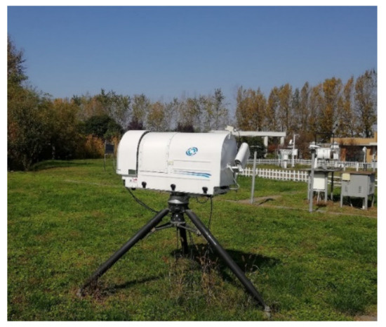
Figure 1.
The microwave radiometer (MWP967KV) used in this experiment.
The upgraded GMR works on two modes: the meteorological observation mode and the solar observation mode. Generally, the GMR works on the meteorological observation mode to observe the atmospheric temperature and humidity profiles.
The solar observation was made by collecting drift scans through the center of the solar disk by using the Polar Plane Indicator (PPI) and Range Height Indicator (RHI) and scanning was conducted by adding the step angle. In addition, a number of scanning points were made to correct for small residual pointing errors. In addition, the antenna was adjusted so that the sun was completely out of path of the beam. The sky was scanned using RHI scanning and these scanning data were used to calibrate the atmospheric opacity at different elevations by using the Tipping method [23].
Since the sun was moving along the sky within the scanning time interval, we needed to re-calculate the solar azimuth and elevation prior to changing the antenna pointing position in real-time. This was used to derive the relative position between the antenna beam pointing position and the sun for each observation. During the experiment, the solar observations were typically performed once or twice a week on sunny days. The sun was observed for more than 3 h a day and the observations were repeated every 10 min.
3. Results
3.1. Mean Radiative Temperature
In order to predict the mean radiative temperature, a regression analysis based on regressions of all of seasons was conducted and we only refer to those regressions performed during clear skies from 2014 to 2019 in Xi’an, China. We could find a correlation between the simulated mean radiative temperature from radiative transfer model and the regression mean radiative temperature from the surface meteorological observations. The regression results are shown in Table 1 and Figure 2. As can be observed, the correlation coefficients of are 0.971, 0.982, and 0.979 for each frequency and the slops are 0.9434, 0.964, and 0.9593; therefore, the fit was slightly worse for the situations with clear-skies.

Table 1.
Regression coefficients and BIAS and RMS of calculating Tm , , , and are the regression coefficients. The BIAS means the mean bias and the RMS means the root-mean-square error.
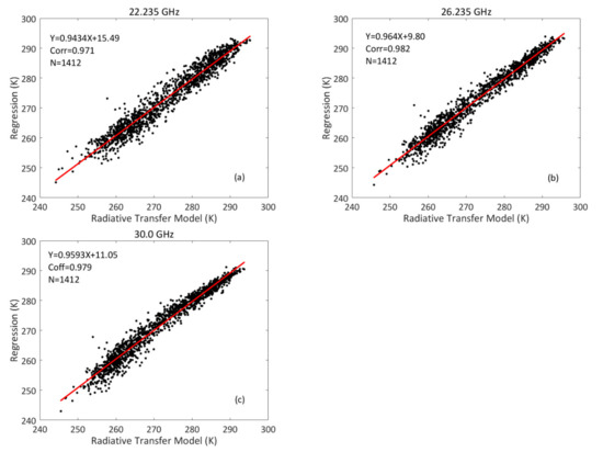
Figure 2.
The mean radiative temperature at different frequencies. A comparison of the regression method and radiative transfer model using the sounding profiles when the sky was clear. The sample size (N), the correlation (Coff), and the fitting are shown. (a) 22.235 GHz, (b) 26.235 GHz, and (c) 30.0 GHz.
Considering the importance of small variations in , we calculated the BIAS and RMS. The results for each of the frequencies are presented in Table 1. The BIAS were 2.09, 1.66, and 1.75 K and the RMS were 2.65, 2.17, and 2.26 with respect to the three frequencies.
3.2. Observation of the Solar TB Increment
On a sunny day, when we scan the sun at a fixed elevation with GMR in azimuth, we can assume that the atmospheric attenuation is a constant and can be easily calculated and calibrated by using Equation (2). Some observation examples at the three frequencies are shown in Figure 3. The results demonstrated that the observation curves (circled by the dashed line) were a Gaussian function and the maximum value indicates that the antenna was pointed to the center of the sun. According to Equation (9), the scanning curve is the antenna pattern. When the sun was scanned by the GMR at an elevation, the antenna azimuth angle was equal to the solar azimuth and it was a fixed value. However, the atmospheric attenuation was not a constant and it had a different value as the antenna elevation. Some elevation scanning examples are shown in Figure 4. Compared with Figure 3, the azimuth and elevation scanning results had some obvious difference that depended on the atmospheric attenuations at different elevation angles. The atmospheric attenuation was more obvious with a lower elevation and it is shown in Figure 4 (blue dotted line).
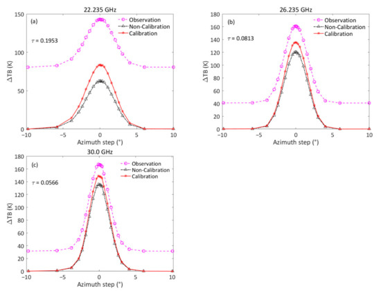
Figure 3.
An example of the solar azimuth scanning observation on 18 June 2020, 12:00 a.m. (local time). The azimuth angle distortion was calibrated. The pink dashed line is the scanning points value. The red solid line is the TB increment after the atmospheric attenuation calibration and the black dash-dotted line is for the observational TB increment without the atmospheric attenuation calibration. The markers represent the observed data and the origin represents the center of the sun. The left axis is the solar TB increments (ΔTB) at different azimuths. (a) 22.235 GHz, (b) 26.235 GHz, and (c) 30.0 GHz.
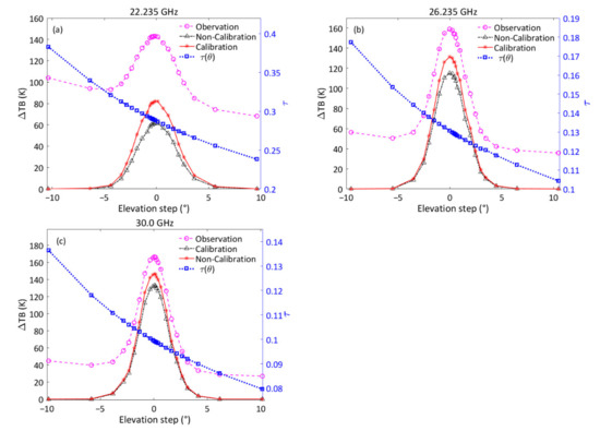
Figure 4.
An example of the solar azimuth scanning observation on 18 June 2020, 17:10 p.m. (local time). The pink dashed line is the scanning point values. The red solid line is the TB increment after the atmospheric attenuation calibration and the black dash-dotted line is for the observational TB increments without the atmospheric attenuation calibration. The blue dotted line is the atmospheric attenuations at different elevations. The markers represent the observed data and the origin represents the center of the sun. The left axis is the solar TB increment (ΔTB) at different elevations and the right axis is the atmospheric opacity (τ) at different elevations. (a) 22.235 GHz, (b) 26.235 GHz, and (c) 30.0 GHz.
During the solar scanning observation, the observed TB increment of the sun was observed after atmospheric attenuation. If we did not calibrate the attenuation, the solar TB increment would be smaller than the real value and this is shown in Figure 3 and Figure 4 (red solid and black dash-dotted lines). In a comparison of the process of the azimuth and elevation scanning, the atmospheric attenuation calibration is obviously important. The scanning results showed the following: (1) The azimuth scanning observation points showed good consistency with the results from a fitting of the Gaussian function. The elevation scanning points were not a perfect Gaussian function and the sky radiation TB and the solar TB increment were larger with a lower elevation (pink dashed line in Figure 4). (2) The maximum value of the solar TB increment was different for each frequency and they were related to the antenna beamwidth. In addition, the TB increment was more obvious with a narrower beamwidth. (3) In order to measure the absolute solar TB, the atmospheric attenuation had to be calculated at different elevations. During the elevation scanning, the results showed good agreement with the Gaussian function after the calibration of the atmospheric attenuation at different elevations (red solid line in Figure 4).
3.3. Measurement of the Antenna Pattern
The GMR antenna pattern measurement is important for an accurate solar TB measurement. We used the GMR to track and scan the sun at various frequencies. Since the beginning of December 2019, sun tracking and monitoring were performed on sunny days. It was found that the GMR could observe the TB increment arising from solar radiation. In order to reduce the impact of the atmospheric refraction and the side lobes of the antenna beam, observations at low elevations were avoided (<25°).
During the observation, the sun can be assumed a point source for the antenna and can be treated as a homogeneous disk with an approximate angular diameter of 0.53°. According to Equation (9), the antenna pattern can be easily fitted by the least-square method by using solar scanning data after calibration of the atmospheric attenuation. During the sun scanning, the atmospheric attenuation is very obvious for the solar radiation and the effect of the attenuation.
After calibrating the atmospheric attenuation, we obtained the solar TB increment when the antenna beam was pointed near the sun and the antenna beamwidth was obtained with the results from a fitting of the Gaussian function. Figure 5 and Figure 6 show some examples of the solar observation values with azimuth and elevation scanning at three frequencies and the antenna pattern could fit in accordance with the Gaussian function. The results showed that the scanning data was relatively symmetrical and the peak TB increment was inversely proportional to the beamwidth.
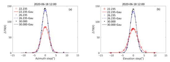
Figure 5.
An example of the solar scanning observation on 18 June 2020, 12:00 a.m. (local time). The angle distortion was calibrated. The solar elevation was 78.1°.The markers are for the observed TB increments and the lines are for fitting with the Gaussian function by using the least-square method. The origin represents the center of the sun. (a) Azimuth scanning and (b) elevation scanning.
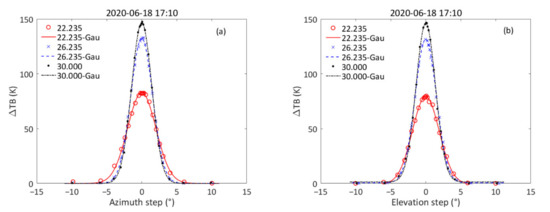
Figure 6.
The same as Figure 5 but for 18 June 2020, 17:10 p.m. (local time). The angle distortion was calibrated and the solar elevation was 31.5°. (a) Azimuth scanning, and (b) Elevation scanning.
In order to study the effect of the different elevations for the scanning observation, we continuously scanned the sun throughout the day at different solar elevation angles. Figure 7 shows the daily variations in the peak TB increments, the beamwidth, and the ratio, R, on 18 June 2020, as shown in Table 2. No elevation dependence of the TB increment, beamwidth, and the ratio, R, could be found. Based on the statistical data, the maximum standard deviation (STD) of the TB increment was 1.54 K at 30.0 GHz and the maximum STD of the beamwidth was 0.1° at 22.235 GHz. The low STD found for the GMR demonstrated the stability of the sun-based monitoring and the GMR receiving system.
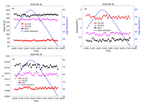
Figure 7.
The daily variation of the maximum TB increment and beamwidth on 18 June 2020. The “Peak TB” is the maximum TB increment when the antenna beam points to the center of the sun. The ratio R is the sun filled-beam factor of the GMR antenna. All times were local time. (a) The maximum TB increment, (b) antenna beamwidth, and (c) the ratio R.
Table 2.
The statistical results of the beamwidth and the ratio of the solar solid angle to the antenna solid angle (R) on 18 June 2020 at the three frequencies. The “Peak TB” is the maximum solar TB increment when the antenna beam was pointed to the center of the sun. The “Mean” and “STD” are the mean value and standard deviation, respectively.
3.4. TB of the Sun
Assuming a uniform disk for the sun, we observed and calculated the absolute TB of the sun, which was analyzed by using the data of the daily mean TB and STD on 18 June 2020. The results of the solar TB are shown in Figure 8 and the statistical daily mean and STD of the solar TB are shown in Table 3. The maximum solar TB was 10,119.3 K at 26.235 GHz, and the maximum STD was 396.9 K at 22.235 GHz. As shown in Table 2, the STD of the beamwidth was also the largest value at 22.235 GHz. Figure 8 shows that the solar TB observation did not depend on the variation in the solar elevation. However, the side lobes of the antenna beam may have received the radiation from the ground at the low elevation. For this reason, solar observations should avoid low elevations.
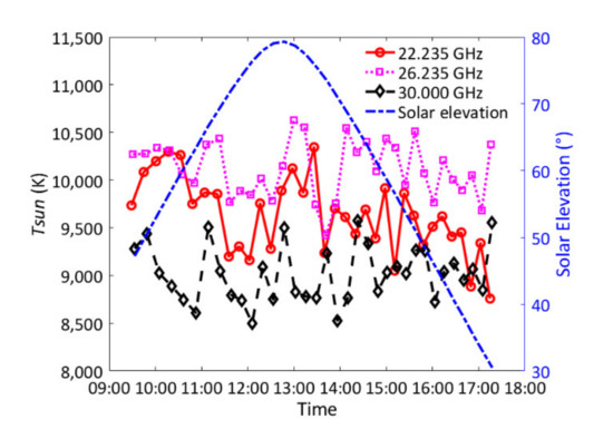
Figure 8.
The variation in the solar TB on 18 June 2020 at 22.235, 26.235, and 30.0 GHz. Tsun is the solar TB.
Table 3.
The statistical results of the solar TB (Tsun) on 18 June 2020 at the three frequencies. The “Mean” and “STD” are the mean value and standard deviation, respectively.
4. Discussion
4.1. Effect of the Mean Radiative Temperature
The mean radiative temperature, , plays a role in many applications of the GMR. The uncertainties in the are typically not a significant factor for zenith observation because the TBs are very small [24]. In a study by Han and Westwater, they presented a comprehensive analysis of the effect of the mean radiative temperature and the regression method provided an observation accuracy of 1.0 K or better for the zenith observation [24]. However, the TB can be large at a low elevation in the Tipping calibration. During the solar observation and considering the sun filled-beam efficiency being less than 0.02, the observation error of the solar TB may be obvious.
Figure 9 shows an example of how the uncertainties affected the observation of the solar TB. In order to evaluate the effect of the , we added some error to the regression . The results showed that the effect was different at different frequencies and when the error of the was 10 K, the solar TB observation error can be around 50–100 K. However, according to our simulation, the uncertainties can be reduced by using the regression method and the solar TB observation error may be less than 50 K. For a solar TB that is over 6000 K, the calibration error can be ignored.
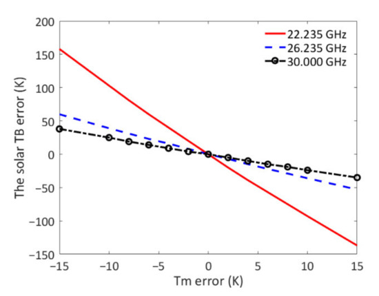
Figure 9.
The mean calibration error on June 18, 2020 at the three frequencies. The calibration errors depend on the mean radiative temperature, Tm. The origin represents the mean radiative temperature according to the regression method, and the error was 0.
4.2. Effect of the Earth-Sun Distance
The orbit of the earth is an ellipse according to the distance between the sun and the earth at the perihelion and aphelion. The Earth-Sun distance varies by approximately 6.5% throughout the year and the angular radius of the sun, , depends on the distance. According to Equation (10) and Equation (11), the ratio, R, can be affected and the Earth-Sun distance is an important factor for the measurement of solar TB.
Figure 10 shows that the ratio, R, varies with the angular radius of the sun and the results showed that the ratio varied by approximately 6.88%, 6.86%, and 6.85% at 22.235, 26.235, and 30.0 GHz, respectively. According to Equation (5) and the TB of the sun, this observation error was very obvious. Therefore, the Earth-Sun distance effect had to be calibrated.
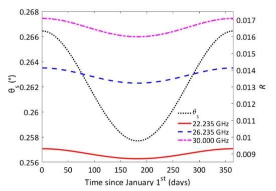
Figure 10.
The ratio, R, varies with the angular radius of the sun throughout the year. is the angular radius of the sun (left axis) and the ratio, R, is the ratio of the solar solid angle to the antenna solid angle (right axis).
4.3. Effect of the Antenna Alignment
The pointing of the antenna beam has an error between the reading of the angle sensor and the actual beam pointing position because of environmental changes and the effect of other factors [35]. During tracking of the sun, the pointing error has to be calibrated and monitored. The traditional calibration methods require other reference sources to calibrate the pointing error, but these traditional methods are expensive and complex. In particular, these methods cannot be used to monitor and calibrate the antenna pointing of a radiometer in operational field applications after installation.
Since the solar position can be accurately predicted, we can calibrate the antenna pointing position by scanning the sun. The calibration angles of the azimuth and elevation are equivalent to the difference between the predicated solar position and the angle measured when the TB received is maximized [35]. The maximum amplitude of the TB increment is received by the GMR when the antenna beam points to the center of the sun. During the beam scanning of the azimuth and elevation, the sun is located using an automatic search method until a maximum TB is found and the pointing bias can be determined by this method. In addition, this result can be used to automatically check and calibrate the pointing of a GMR antenna that is deployed in the field.
Pointing errors can impact the accuracy of the Tipping calibration, but the effect of the pointing error can be reduced by performing the Tipping observation on both sides and the uncertainties caused by a 1° pointing error can be reduced to approximately 0.1° [21]. However, the pointing error cannot be ignored for sun tracking observations. According to the measured antenna pattern in Section 3.3, the solar TB observation error can be simulated. The simulated results showed that the pointing error and the beamwidth dependence of the solar TB increment could be found at each frequency and the uncertainties in the pointing error may cause a significant observation error for the solar TB. The solar TB observation error could be over 20% when the pointing error is around 1°, but if the pointing error is less than 0.2°, the observation error could not exceed 1%. Thus, the pointing error must be calibrated.
In order to further reduce the influence of the pointing error, the solar radiation fluctuation, the observation uncertainty, and the observed TB of the sun by scanning the azimuth and elevation should be fitted by using the least-square method. This can help us to obtain the maximum value position more accurately. In the calibration experiment, we iteratively corrected the azimuth angle and then corrected the elevation angle. Figure 11 shows the real scanning data and the Gaussian fitting curve by using the least-square method and the offset angle can be obtained at the azimuth and elevation. The results showed that the offset angles were different at each frequency. After calibration by using the solar scanning method, the pointing error was less than 0.2° and the effect of the pointing error for the observation can often be reduced significantly [21]. The observation results showed that the solar radiation can be used for monitoring and calibrating the alignment of the GMR antenna.
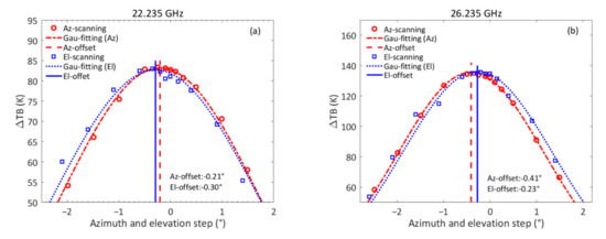
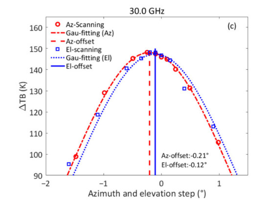
Figure 11.
The real solar scanning and calibrating examples at 22.235, 26.235, and 30.0 GHz and the Gaussian fitting curve using the least-square method. The “Az” and “El” mean the antenna azimuth and elevation, respectively. The “Gau-fitting” means the Gaussian fitting curve using the least-square method. “Offset” means the offset angle of the antenna pointing. The horizontal axis is the rotation angle of the GMR antenna for the azimuth and elevation and the origin represents the center of the sun. The vertical axis is the TB increment. (a)22.35 GHz, (b) 26.235 GHz, and (c) 30.0 GHz.
4.4. Calibration of the Angle Distortion in the Azimuth
When the antenna scans the sun in the azimuth, a rotation of the antenna in the azimuth with a constant elevation is not a great circle in the sky-sphere. The rotation angle is greater than the true azimuth angle in the sky-sphere and there are some distortions in the scanning path [30]. The distortion is more obvious when the antenna elevation increases and it has to be calibrated. Reimann and Hagen studied the calibration method [27] and we calculated the distortion angle by using their method. The results showed that the distortion was small for low-elevation and small-angle rotations in the azimuth. After calibration of the angle distortion, the scanning results were in relatively good agreement at the different solar elevations, as shown by the dashed line in Figure 12.
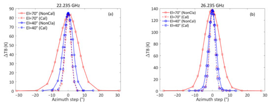
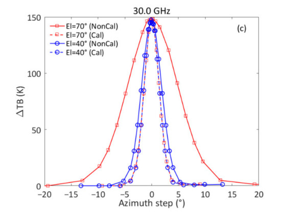
Figure 12.
This is a real example of the scanning angle distortion on 18 June 2020. The azimuth distortion arises from the rotation of the antenna in the azimuth at different solar elevations (40° and 70°). The horizontal axis is the rotation angle of the GMR antenna in the azimuth and the origin represents the center of the sun. The vertical axis is the TB increment. “NonCal” means “before distortion calibration” and “Cal” means “after distortion calibration”. (a) 22.235 GHz, (b) 26.235 GHz, and (c) 30.0 GHz.
According to the simulation result, if we do not calibrate the angle distortion, it can cause a large bias in the beamwidth measurement. Furthermore, the ratios, R, of the solar solid angle to the antenna solid angle and to the calibrated TB of the sun were affected.
4.5. Atmospheric Refraction and the Non-Stratified Atmospheric Condition
During the observation, the observed radiation of the sun was refracted during its propagation through the atmosphere. The atmospheric refraction causes the beam to bend downwards under normal conditions and the antenna azimuth bias does not depend on the refraction. Therefore, the refraction introduces a bias in the solar position and this has to be considered, especially at a low elevation. Huuskonen and Holleman studied the atmospheric refraction model [36] and we can calculate the refraction from their calculation model. In addition, the effect of the refraction for the beam can often be calibrated during the solar scanning observation.
In this study, the refraction curves have been calculated by using different elevations for the U.S. Standard Atmosphere, 1976, and this is shown in Figure 13. The results showed that the atmospheric refraction had a significant influence on the beam pointing, especially for the antenna pointing at the lower elevation. In addition, the radiometer did not have an infinitesimal beamwidth and the side lobes of the antenna beam may have picked up radiation at a low elevation from the ground source. Figure 13 shows that the refraction angle was less than 0.05° when the antenna elevation was greater more than 20°. In the Han and Westwater study [21], this effect could be ignored. For these reasons, a solar observation should avoid low elevation angles.
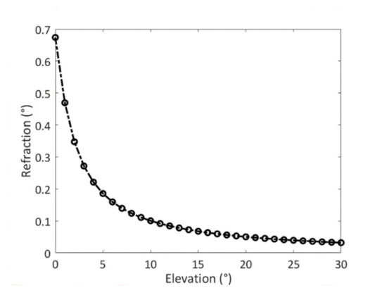
Figure 13.
The refraction curve as a function of elevation was calculated by using the refraction model. The interval between data points is fixed (1°) on the horizontal axis.
During the observation, the Tipping curve calibration and the refraction calibration requires a horizontally stratified atmosphere. This is the reason why the Tipping calibration is typically performed under clear-sky conditions [24]. Therefore, the solar observations were performed on sunny days.
Due to the spatial variations in the cloud and the horizontal inhomogeneity of the water vapor, a large observation uncertainty is produced under a cloudy-sky condition, especially for middle and low clouds. According to our experiment, the effect was not obvious for a high cloud. In order to reduce the effect of a non-stratified atmosphere, observations should be avoided at low elevations.
4.6. Long-Term Observation
Figure 14 shows the annual variation of the daily mean beamwidth, the ratio of the solar solid angle to the antenna solid angle and the solar TB from December 2019 to February 2021 at the three frequencies. The statistical annual mean and standard deviation of the beamwidth and the ratio, R, are shown in Table 4. The results showed that the beamwidth was less than 5°at each frequency. By comparing the difference between the solar method and the traditional method, the difference between the two methods was less than 0.1°. The results of the measurement indicated that the measured beamwidth matched well to the pattern based on the traditional method and the antenna complied with the design specification [21]. The experimental results showed that the method of the antenna pattern measurement based on solar observations had the advantages of simple operation and feasibility in the field.
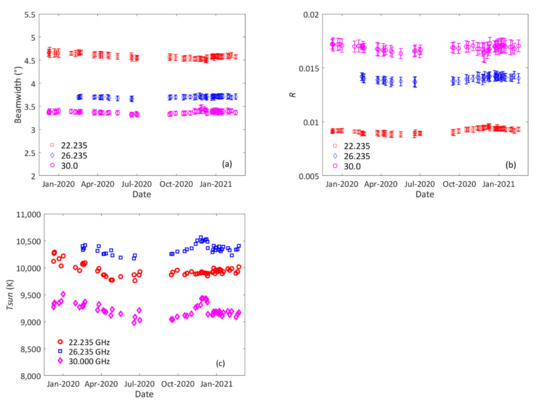
Figure 14.
The annual variation of the daily mean beamwidth, the ratio R, and solar TB. The ratio, R, is the solar solid angle to the antenna solid angle and Tsun is the solar TB at the different frequencies. The markers are the observed daily means. (a) Beamwidth, (b) he ratio R, and (c) the daily mean solar TB.
Table 4.
The statistical results of the beamwidth, the ratio of the solar solid angle to the antenna solid angle (R), and the solar TB (Tsun) from December 2019 to February 2021 at the three frequencies.
After measuring the antenna beamwidth, we calculated the ratio, R, of the solar solid angle to the antenna solid angle according to the Earth-Sun distance and Equation (5). This was based on the calculation the absolute TB of the sun. The antenna pattern characteristics are the most significant factor that affects the estimation. The result showed that the proportion of the sun in the GMR antenna beam was less than 2% at the three frequencies and the ratio was inversely proportional to the beamwidth.
Figure 14 and Table 4 show the annual variation of the daily mean TBs of the sun and the STD from December 2019 to February 2021 at the three frequencies. The TBs of the sun obtained were 9950 ± 334, 10,351 ± 370, and 9217 ± 375 K at 22.235, 26.235, and 30.0 GHz, respectively. The scans under different solar elevations and seasons have been completed in order to study the effect of the solar elevation and seasonal variation on the measurement TBs of the sun and the seasonal and elevation dependence is not obvious.
Figure 14 shows a long time series of solar observations. These results showed the variation of the solar radiation at the different solar elevations and seasons and the measurement results did not have obvious seasonal variations. The long-term observation showed that the method can be used throughout the year. For long-term observations, a little fluctuation in the beamwidth and the ratio, R, demonstrated the long-term stability of the GMR receiving system. This can be used to evaluate the stability of the radiometer according to the previous results [1,21,28,29,37,38]. Therefore, we can observe that the solar radiation observation was revealed to be potentially useful for a GMR system assessment. A long time series of the solar brightness temperature estimates can provide better confidence in the performed estimates that use a GMR.
The TB of the quiet sun has been measured at many frequencies in the microwave band, and the measured results are summarized in papers published by Shimabukuro and Stacey [39]. In order to obtain better comparisons, the measured TB of the sun from 15 to 54.5 GHz were compiled and are plotted in Figure 15. In particular, K-band measurements were available from previous literature [1,37,39]. The results showed that (1) a comparison of the TB at 22.235 GHz with the previous results at 22 and 23.4 GHz showed that the average percentage deviation was 9.1%. (2) A comparison of the TB at 26.235 GHz with the previous result at 25.4 GHz showed that the average percentage deviation was 5.3%. (3) A comparison of the TB at 30.0 GHz with the previous result at 31.4 GHz showed that the average percentage deviation was 4.5%. The results were in relatively good agreement with those found in the literature [1,39]. Mattioli et al. obtained the same results and they also obtained a large percentage deviation at low-frequency [1]. The TB of the sun showed a decreasing behavior with frequency values from approximately 10,000 K down to approximately 6000 K from 15 GHz to 55 GHz, as shown in Figure 15. In addition, the statistical results showed that the measured STD of the solar TB obtained by using the GMR was less than that of former researchers’ results and this result showed that the measured solar TBs obtained from the GMR were more stable.
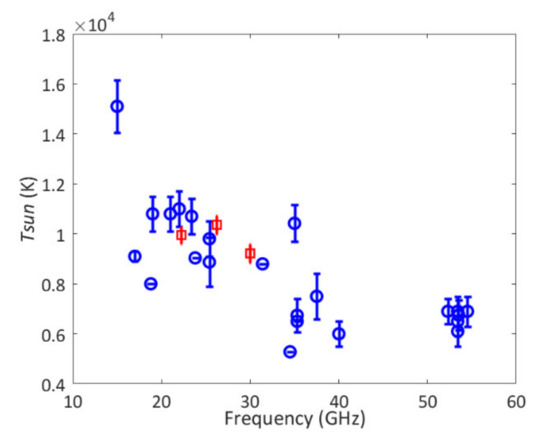
Figure 15.
The solar TB versus frequency. The red rectangle represents the mean solar TB observed by the GMR. The blue circle represents the mean TB summarized by Shimabukuro and Stacey (1968) and Mattioli et al. (2016). Tsun is the solar TB and the error bar represents the standard deviation. Some circles have zero standard deviation because the paper did not give the standard deviation in literature.
4.7. Effect of the Solar Activity
During a long-term observation, we can observe that the TB of the sun is not constant (see Figure 14c). This is because the solar radiation intensity varies on a daily basis and it depends on the solar activity [30]. The sunspot number is a widely-used index of solar activity [31,40]. By comparing the daily mean and the STD of the solar TB with the sunspot number, we found that the daily mean and STD increased significantly in November and December 2020. The obvious variation may have arisen due to the solar activity and because there were many sunspots during these times, as shown in Figure 16. There was a slight correlation between solar activity and solar radiation and a variation from solar activity has been observed in the microwave band [26,41,42,43,44].
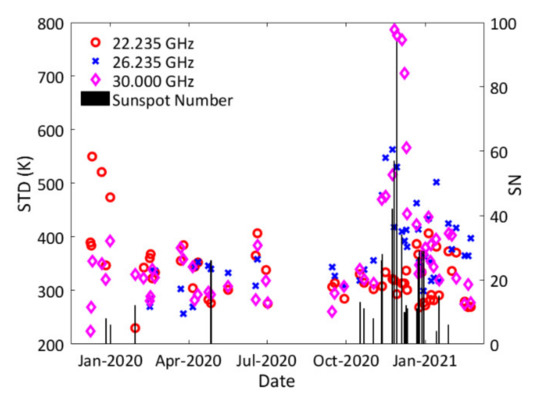
Figure 16.
The correlation between the daily standard deviation (STD) of the solar TB and the sunspot numbers (SN) (Source: WDC-SILSO, Royal Observatory of Belgium, Brussels).
In this study, the TBs of the sun exhibited a slight increase during the solar active episode and the variation was more obvious with a narrower beamwidth at 26.235 and 30.0 GHz (see Figure 14c and Figure 16). We found that the variations in the STD and the daily TB of the sun were more obvious with an increased number of sunspots of greater than 20. That is to say that the fluctuation in the solar TB significantly increased during the solar active episode and this indicated a better sensitivity of the receiver. This demonstrated that, even during active solar episodes, the operational GMR could accurately monitor the radiation signal of the sun. In addition, the sunspots had no obvious effect when measuring the beamwidth and the ratio R (see Figure 14a,b and Figure 15).
In order to study the correlation between the solar TB and the sunspot number, the observation data was fitted with a logarithmic function. A positive relationship existed between the solar TB and the sunspot number, as shown in Figure 17. Hence, the solar observation by the GMR demonstrated a potential application for predicting the sunspot number.
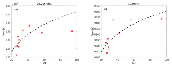
Figure 17.
Correlation between the solar TB and the sunspot number. Tsun is the solar TB and SN is the sunspot number. The dash line is logarithm trend-line fitting; (a) 26.235 GHz and (b) 30.0 GHz.
5. Conclusions
In this paper, we introduced an application for tracking and observing the sun that utilizes the GMR. Based on the theory of thermal radiation and its transfer in the atmosphere, we provided a convenient method to measure the absolute TB of the sun by using observations from the GMR. This method featured simple computation and it obtained results that had close accuracy with other results. Furthermore, we improved the antenna servo control system of the GMR so that it could be used to track and scan the sun. We conducted a long-term attempt to scan and observe the sun by using the upgraded GMR at a Xi’an field experimental site from December 2019 to February 2021.
During the observation, we found that the solar observation method can be used to measure the solar TB increment, the antenna pattern, and the sun filled-beam factor of the GMR antenna at different frequencies. Based on the results, the TB of the sun can be accurately measured by using the GMR at multi-frequency levels. The results showed that the TBs of the sun were 9748 ± 340, 10,240 ± 365, and 9185 ± 370 K at 22.235, 26.235 and 30.0 GHz, respectively. In order to validate our results, the estimated TB of the sun was compared with the previous results from the literature and the results showed that we had obtained average percentage deviations of 9.1%, 5.3%, and 4.5% at 22.235, 26.235, and 30.0 GHz, respectively. These results were consistent with those of previous research.
In order to study the long-term variation in the solar TB, the annual and daily variations in the TB of the sun were analyzed at three frequencies. According to the daily TB of the sun variations, the TB of the sun was not a constant at each frequency and it had a slight fluctuation that the GMR could respond to. In addition, we found that the GMR could also respond to the variation in the sunspots during active episodes and a positive relationship existed between the solar TB and the sunspot number. In addition, the sunspots did not have an obvious effect on the antenna pattern measurement.
By utilizing this method, it was possible to determine the TB of the sun and monitor the solar radiation with the GMR. This means that the GMR can be used to not only observe the atmosphere, but also to monitor the sun. Additionally, the solar radiation method is potentially useful for a GMR system stability assessment. This method develops and extends the application field of the GMR and this will impel the utilization of GMR for monitoring variations in solar microwave radiation.
Author Contributions
Conceptualization, L.L., J.L., and Z.W.; methodology, L.L., J.L., Z.W., and Y.M.; software, L.L..; validation, L.L., L.Z., R.C. and J.Q.; formal analysis, L.L.; resources, L.Z. and R.C.; data curation, L.L.; writing—original draft preparation, L.L., Z.W., and Y.M.; writing—review and editing, L.L., Y.M., and Z.W.; project administration, Z.W. and J.L.; funding acquisition, Z.W. All authors have read and agreed to the published version of the manuscript.
Funding
This research was funded by the National Natural Science Foundation of China (NO.41675028), the Natural Science Foundation of Shanxi Province, China (NO.2020JM-718), the Xi’an Science and Technology Project of Shanxi Province, China (NO. 20SFSF0015), and A Project Funded by the Priority Academic Program Development of Jiangsu Higher Education Institutions (PAPD).
Institutional Review Board Statement
Not applicable.
Informed Consent Statement
Not applicable.
Data Availability Statement
The data presented in this study are available on request from the corresponding author.
Acknowledgments
We are grateful to the Shanxi Provincial Atmospheric Sounding Technical Support Center and Xi’an Meteorological Observation Center of Shaanxi Province, China, for the radiometer installation and for their support.
Conflicts of Interest
The authors declare no conflict of interest.
References
- Mattioli, V.; Milani, L.; Magde, K.M.; Brost, G.A.; Marzano, F.S. Retrieval of Sun Brightness Temperature and Precipitating Cloud Extinction Using Ground-Based Sun-Tracking Microwave Radiometry. IEEE J. Sel. Top. Appl. Earth Obs. Remote. Sens. 2016, 10, 3134–3147. [Google Scholar] [CrossRef]
- Ulich, B.L. Absolute brightness temperature measurements at 2.1-mm wavelength. Icarus 1974, 21, 254–261. [Google Scholar] [CrossRef]
- Gabella, M.; Huuskonen, A.; Sartori, M.; Holleman, I.; Boscacci, M.; Germann, U. Evaluating the Solar Slowly Varying Component at C-Band Using Dual- and Single-Polarization Weather Radars in Europe. Adv. Meteorol. 2017, 2017, 4971765. [Google Scholar] [CrossRef]
- Iwai, K.; Shimojo, M.; Asayama, S.; Minamidani, T.; White, S.; Bastian, T.; Saito, M. The Brightness Temperature of the Quiet Solar Chromosphere at 2.6 mm. Sol. Phys. 2017, 292, 22. [Google Scholar] [CrossRef]
- Ulich, B.; Haast, R. Absolute calibration of millimeter-wavelength spectral line. Astrophys. J. Suppl. Ser. 1976, 30, 247–258. [Google Scholar] [CrossRef]
- Ulich, B.; Davis, J.; Rhodes, P.; Hollis, J. Absolute brightness temperature measurements at 3.5-mm wavelength. IEEE Trans. Antennas Propag. 1980, 28, 367–377. [Google Scholar] [CrossRef]
- Kosugi, T.; Ishiguro, M.; Shibasaki, K. Polar-cap and coronal-hole-associated brightenings of the sun at millimeter wavelengths. Publ. Astron. Soc. Jpn. 1986, 38, 1–11. [Google Scholar]
- White, S.M.; Loukitcheva, M.; Solanki, S.K. High-resolution millimeter-interferometer observations of the solar chromosphere. Astron. Astrophys. 2006, 456, 697–711. [Google Scholar] [CrossRef]
- Ahn, M.-H.; Won, H.Y.; Han, D.; Kim, Y.-H.; Ha, J.-C. Characterization of downwelling radiance measured from a ground-based microwave radiometer using numerical weather prediction model data. Atmos. Meas. Tech. 2016, 9, 281–293. [Google Scholar] [CrossRef]
- Bianco, L.; Friedrich, K.; Wilczak, J.M.; Hazen, D.; Wolfe, D.; Delgado, R.; Oncley, S.P.; Lundquist, J.K. Assessing the accuracy of microwave radiometers and radio acoustic sounding systems for wind energy applications. Atmos. Meas. Tech. 2017, 10, 1707–1721. [Google Scholar] [CrossRef]
- Cadeddu, M.P.; Liljegren, J.C.; Turner, D.D. The atmospheric radiation measurement (ARM) program network of microwave radiometers: Instrumentation, data, and retrievals. Atmos. Meas. Tech. 2013, 6, 2359–2372. [Google Scholar] [CrossRef]
- Xu, G.; Xi, B.; Zhang, W.; Cui, C.; Dong, X.; Liu, Y.; Yan, G. Comparison of atmospheric profiles between microwave radiometer retrievals and radiosonde soundings. J. Geophys. Res. Atmos. 2015, 120, 10313–10323. [Google Scholar] [CrossRef]
- Yang, J.; Min, Q. Retrieval of atmospheric profiles in the New York State Mesonet using one-dimensional variational algorithm. J. Geophys. Res. Atmos. 2018, 123, 7563–7575. [Google Scholar] [CrossRef]
- Cimini, D.; Rosenkranz, P.W.; Tretyakov, M.Y.; Koshelev, M.; Romano, F. Uncertainty of atmospheric microwave absorption model: Impact on ground-based radiometer simulations and retrievals. Atmos. Chem. Phys. Discuss. 2018, 18, 15231–15259. [Google Scholar] [CrossRef]
- Caumont, O.; Cimini, D.; Löhnert, U.; Alados-Arboledas, L.; Bleisch, R.; Buffa, F.; Ferrario, M.E.; Haefele, A.; Huet, T.; Madonna, F.; et al. Assimilation of humidity and temperature observations retrieved from ground-based microwave radiometers into a convective-scale NWP model. Q. J. R. Meteorol. Soc. 2016, 142, 2692–2704. [Google Scholar] [CrossRef]
- Che, Y.; Ma, S.; Xing, F.; Li, S.; Dai, Y. An improvement of the retrieval of temperature and relative humidity profiles from a combination of active and passive remote sensing. Meteorol. Atmos. Phys. 2018, 131, 681–695. [Google Scholar] [CrossRef]
- Wang, Z.; Li, Q.; Hu, F.; Cao, X.; Chu, Y. Remote sensing of lightning by a ground-based microwave radiometer. Atmos. Res. 2014, 150, 143–150. [Google Scholar] [CrossRef]
- Jiang, S.; Pan, Y.; Lei, L.; Ma, L.; Li, Q.; Wang, Z. Remote sensing of the lightning heating effect duration with ground-based microwave radiometer. Atmos. Res. 2018, 205, 26–32. [Google Scholar] [CrossRef]
- Jiang, S.; Wang, Z.; Lei, L.; Pan, Y.; Lyu, W.; Zhang, Y. Preliminary study on the relationship between the brightness temperature pulses observed with a ground-based microwave radiometer and the lightning current integral values. Atmos. Res. 2020, 245, 105072. [Google Scholar] [CrossRef]
- Marzano, F.S.; Mattioli, V.; Milani, L.; Magde, K.M.; Brost, G.A. Sun-Tracking Microwave Radiometry: All-Weather Estimation of Atmospheric Path Attenuation at Ka-, V-, and W-Band. IEEE Trans. Antennas Propag. 2016, 64, 4815–4827. [Google Scholar] [CrossRef]
- Lei, L.; Wang, Z.; Qin, J.; Zhu, L.; Chen, R.; Lu, J.; Ma, Y. Feasibility for Operationally Monitoring Ground-Based Multichannel Microwave Radiometer by Using Solar Observations. Atmosphere 2021, 12, 447. [Google Scholar] [CrossRef]
- D’Orazio, A.; de Sario, M.; Gramegna, T.; Petruzzelli, V.; Prudenzano, F. Optimisation of tipping curve calibration of microwave radiometer. Electron. Lett. 2003, 39, 905. [Google Scholar] [CrossRef]
- Han, Y.; Westwater, E. Analysis and improvement of tipping calibration for ground-based microwave radiometers. IEEE Trans. Geosci. Remote. Sens. 2000, 38, 1260–1276. [Google Scholar] [CrossRef]
- Zhang, M.; Gong, W.; Ma, Y.; Wang, L.; Chen, Z. Transmission and division of total optical depth method: A universal calibration method for Sun photometric measurements. Geophys. Res. Lett. 2016, 43, 2974–2980. [Google Scholar] [CrossRef]
- Schneebeli, M.; Mätzler, C. A calibration scheme for microwave radiometers using tipping curves and Kalman filtering. IEEE Trans. Geosci. Remote Sens. 2009, 47, 4201–4209. [Google Scholar] [CrossRef]
- Coates, R. Measurements of Solar Radiation and Atmospheric Attenuation at 4.3-Millimeters Wavelength. Proc. IRE 1958, 46, 122–126. [Google Scholar] [CrossRef]
- Ulich, B. A radiometric antenna gain calibration method. IEEE Trans. Antennas Propag. 1977, 25, 218–223. [Google Scholar] [CrossRef]
- Holleman, I.; Huuskonen, A.; Kurri, M.; Beekhuis, H. Operational Monitoring of Weather Radar Receiving Chain Using the Sun. J. Atmos. Ocean. Technol. 2010, 27, 159–166. [Google Scholar] [CrossRef]
- Altube, P.; Bech, J.; Argemí, O.; Rigo, T.; Pineda, N. Intercomparison and Potential Synergies of Three Methods for Weather Radar Antenna Pointing Assessment. J. Atmos. Ocean. Technol. 2016, 33, 331–343. [Google Scholar] [CrossRef]
- Reimann, J.; Hagen, M. Antenna Pattern Measurements of Weather Radars Using the Sun and a Point Source. J. Atmos. Ocean. Technol. 2016, 33, 891–898. [Google Scholar] [CrossRef]
- Tapping, K.F. The 10.7cm solar radio flux (F10.7). Space Weather 2013, 11, 394–406. [Google Scholar] [CrossRef]
- Lahaye, T. Measuring the eccentricity of the Earth’s orbit with a nail and a piece of plywood. Eur. J. Phys. 2012, 33, 1167–1178. [Google Scholar] [CrossRef][Green Version]
- Yu, F.J. Calculating the eccentricity of the Earth’s orbit by approximate orbital equation. Coll. Phys. 2017, 36, 23–24. (In Chinese) [Google Scholar]
- Renju, R.; Raju, C.S.; Mathew, N.; Antony, T.; Moorthy, K.K. Microwave radiometer observations of interannual water vapor variability and vertical structure over a tropical station. J. Geophys. Res. Atmos. 2015, 120, 4585–4599. [Google Scholar] [CrossRef]
- Qi, X.; Wang, J.; Zhao, L.; Ji, J. Antenna beam angle calibration method via solar electromagnetic radiation scan. J. Eng. 2019, 2019, 7890–7893. [Google Scholar] [CrossRef]
- Huuskonen, A.; Holleman, I. Determining Weather Radar Antenna Pointing Using Signals Detected from the Sun at Low Antenna Elevations. J. Atmos. Ocean. Technol. 2007, 24, 476–483. [Google Scholar] [CrossRef]
- Darlington, T.; Kitchen, M.; Sugier, J.; de Rohan-Truba, J. Automated real-time monitoring of radar sensitivity and antenna pointing accuracy. In Proceedings of the 31st Conference on Radar Meteorology, Seattle, WA, USA, 6–12 August 2003; pp. 538–541. [Google Scholar]
- Gabella, M.; Leuenberger, A. Dual-Polarization Observations of Slowly Varying Solar Emissions from a Mobile X-Band Radar. Sensors 2017, 17, 1185. [Google Scholar] [CrossRef] [PubMed]
- Shimabukuro, F.I.; Stacey, J.M. Brightness temperature of the quiet Sun at centimeter and millimeter wavelengths. Astrophys. J. 1968, 152, 777–782. [Google Scholar] [CrossRef]
- Xiao, Q.; Wang, S.; Zhang, Z.; Xu, J. Analysis of Sunspot Time Series (1749–2014) by Means of 0–1 Test for Chaos Detection. In Proceedings of the 2015 11th International Conference on Computational Intelligence and Security (CIS), Shenzhen, China, 19–20 December 2015; pp. 215–218. [Google Scholar] [CrossRef]
- Covington, A.E. Micro-Wave Solar Noise Observations During the Partial Eclipse of November 23, 1946. Nature 1947, 159, 405–406. [Google Scholar] [CrossRef]
- Kaufmann, P.; Scalise, E.; Dos Santos, P.M.; Schaal, R.E.; Fortunato, R.A.A. Microwave observations of the 4 January, 1973 solar eclipse. Sol. Phys. 1973, 33, 69–73. [Google Scholar] [CrossRef]
- Chatterjee, T.N.; Datta, S.K.; Datta, A.K.; Chatterjee, S.; Tarafdar, G.; Bera, J.; Rahman, M.; Bera, R.; Mitra, A.; Karmakar, P.K.; et al. Observation of microwave radio Sun during total solar eclipse on October 24, 1995 by Eastern Centre for Research in Astrophysics (ECRA). Indian J. Phys. Sect. B 1996, 70, 169–173. [Google Scholar]
- Sawant, H.S.; Srivastava, N.; Trigoso, H.E.; Sobral, J.H.A.; Fernandes, F.C.R.; Cecatto, J.R.; Subramanian, K.R. Radio Observation of Total Solar Eclipse of November 3, 1994 at Chapecoó (BRZIL). Adv. Space Res. 1997, 20, 2359–2363. [Google Scholar] [CrossRef]


Publisher’s Note: MDPI stays neutral with regard to jurisdictional claims in published maps and institutional affiliations. |
© 2021 by the authors. Licensee MDPI, Basel, Switzerland. This article is an open access article distributed under the terms and conditions of the Creative Commons Attribution (CC BY) license (https://creativecommons.org/licenses/by/4.0/).