Abstract
Nowadays, uncertainties related to the determination of ocean tides remain a major issue for the exploitation of altimetry data in coastal areas. Using Sea Surface Height (SSH) observations from a new GNSS-based system mounted on an Unmanned Surface Vehicle (USV), we develop a crossover methodology to assess tide models under altimetry tracks. To this purpose, we address the Pertuis Charentais area, a semi enclosed sea located in the centre of the Bay of Biscay (France), as a field and modelling case study. We have developed a barotropic model configuration, based on SCHISM platform, using tidal elevations of an up-to-date regional atlas as boundary conditions. To test the impact of boundary conditions, we propose a second configuration where we applied uniform empirical biases in phases and amplitudes on M3 and MN4 constituents. In addition, the survey was designed to highlight the contribution of third and fourth-diurnal waves that are strongly amplified on the shelf and is used to assess model performances under the pass 216 of Sentinel-3A. Our results show that the second configuration reduces the Root-Mean-Square Error (RMSE) of the survey crossover residuals by more than 60%, leading to half of the residuals below 2.5 cm. This improved solution also reduces by 20% the RMSE computed with data from tide gauges located in the inner part of the Pertuis Charentais. Therefore, our study reinforces the importance for coastal tide modelling of an accurate tidal forcing, especially for shallow water waves. We finally discuss the impact of the remaining M4 error on crossover residual heights. By introducing an empirical correction term based on M4 observations at tide gauges, we further reduce the RMSE of crossover residuals by 15–25%. With this innovative study, we demonstrate the interest of combining crossover validation methods and USV systems to spatially extend our understanding of coastal areas dynamics. This will be crucial in the scope of the future SWOT mission, for which the tide correction accuracy must be assessed over the large-extent areas covered by swaths observations.
1. Introduction
Satellite altimetry recently reached an unprecedented level of global coverage with seven missions flying simultaneously. While altimeters have been originally designed for open ocean and have improved our understanding of the large-scale ocean dynamic, the exploitation of coastal altimetry data remains a challenge that mobilizes a large effort in the scientific community. The future Surface Water Ocean Topography (SWOT) mission [1,2] will help to solve this issue and certainly revolutionize our view of the coastal waters by mapping Sea Surface Height (SSH) with an unprecedented spatial resolution. Based on a radar altimeter sending pulses over a surface, classical nadir altimeters (e.g., Jason series) suffer from their large inherent footprint, which perturbates the reflected signal in the presence of land from 10–15 km from coast [3]. Ka-band altimeter (SARAL) and the next generation of Ku-band SAR altimeters (CryoSat-2 and Sentinel-3) have brought the satellite altimetry observations closer to the shore, thanks to a reduced footprint and an enhanced data/L1 processing [4,5]. However, the across track-resolution remains similar to conventional altimeters and the elongated footprint (even if smaller) makes the incidence angle between the satellite track and the shore an important factor for the land contamination issue [5].
The launch of SWOT scheduled in 2022 will improve the spatial coverage by providing 2D SSH fields. The two-dimensional wide swath observations of the ocean surface topography will be performed by SAR interferometry technique based on two SAR antenna separated by a 10 m mast [1]. The benefit will be substantial in coastal zones in regards of the small size of the resolved pixels (on the order of 50 m), which will allow measurements without land contamination. In the nearshore zone, the standard open ocean product will purpose observations at 2 × 2 km resolution, every 2 km with 2 cm of SSH error. In the coastal area, a native resolution of one pixel of 250 m × 250 m every 250 m, will also be available. With the higher spatial resolution “hydrology” product, observations at a finer scale grid will be available in two resolutions (100 m and 250 m), with larger errors (45 cm error in SSH at 100 m2) [6]. Although spatial averaging will be required to reduce its errors, the use of this high-resolution product will improve the restitution of nearshore dynamics at an unprecedented level. Combined to the high spatial coverage, it makes these wide-swath sea-level observations a unique opportunity to study the fine-scale coastal ocean dynamic.
Despite considerable technological advances, one challenging aspect of coastal altimetry is the lack of accuracy in geophysical corrections, which are critical to derive accurate sea-surface height anomalies (SSHA) near the coast. Especially, uncertainties in ocean tide is still a major issue for the exploitation of altimetry in nearshore regions. Most of the time, the tide correction included in altimetry products is derived from global models, for which the accuracy tends to decrease near the coast, in spite of considerable progress over the last decade [7]. Difficulties encountered in modelling the coastal tide are mainly due to its non-linear behaviour caused by changes in depth, shoreline interactions, or varying bottom drag as it propagates onto shallower waters. The distortion of tidal propagation can thus be represented as additional tidal waves, referred to as overtides (e.g., M4 due to the interaction of M2 with itself, or M6 mainly due to the interaction of M2 with M4) or compound tides (resulting from interactions between two or more constituents, e.g., MN4 or MS4) [8]. These interactions are numerous, and a great number of constituents have to be considered in order to accurately reproduce the full tidal signal in shallow regions. Consequently, efforts in developing regional modelling of coastal areas are encouraged, as well as the consideration of ocean/shelf/land as a modelling continuum, for the preparation and exploitation of the future SWOT mission [9]. Considering the small periods and wavelengths associated with the shallow water waves, there is a critical need for observations with short space and time scales to appreciate their spatial variability. While tide models are classically validated against tide gauges confined to the coast, new spatially-extended validation capabilities are emerging with the development of mobile GNSS-based systems. They were originally designed to determine the precise marine geoid and thus link measurements of satellite altimeters to a coastal tide gauge [10,11,12]. Recently, Chupin et al. [13] have demonstrated the ability of the Cyclopée system (a combination of a GNSS antenna and an acoustic altimeter) by mounting an Unmanned Surface Vehicle (USV) to map SSH while in motion. At a fixed point, this system provides similar accuracy than the best tide gauge systems and is therefore a way to expend accurate in-situ observations toward satellite ground tracks.
In this paper, we demonstrate the potential of this new SSH mapping system for assessing tide corrections under altimetry tracks, through a methodology based on crossover measurements. To this end, we address the Pertuis Charentais area, a semi enclosed sea located in the centre of the Bay of Biscay, as a field and modelling case study. A new hydrodynamic model based on SCHISM configuration [14] is developed for the region and described in Section 3.4. Two model configurations, which differ by their tidal forcing, are proposed, and compared in this study. We then assess both model performances against coastal tide gauges and through the crossover measurements methodology developed in this study under the pass 216 of Sentinel-3A, in the Pertuis Charentais.
2. Study Area
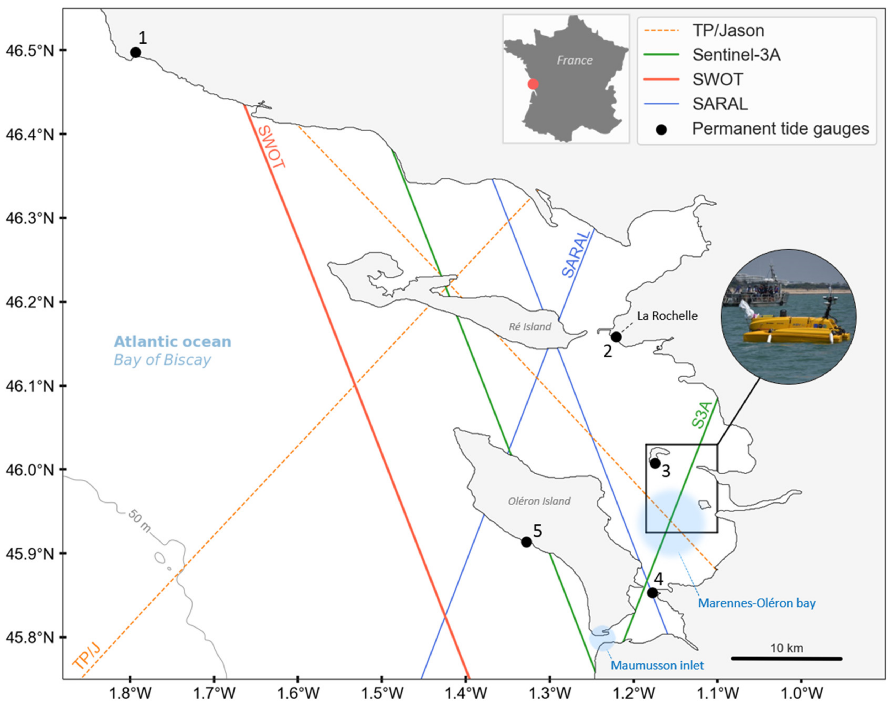
Located in the centre of the French Atlantic coast, in the Bay of Biscay, the Pertuis Charentais area is a sheltered mesotidal coastal zone composed of estuaries, semi-enclosed seas and Islands (Ré and Oléron being the bigger ones, see Figure 1). This particular situation makes it a rich and complex coastal area, which represents a challenge for the exploitation of altimetry measurements as for the good reproducibility of tidal processes by hydrodynamic models.
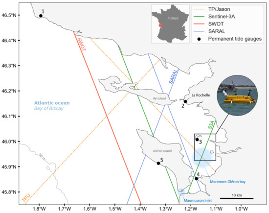
Figure 1.
Overview of the main nominal altimetry tracks and permanent tide gauges in the Pertuis-Charentais area. Permanent tide gauges are represented by black dots: 1—Les Sables d’Olonne (LSDO), 2—La Rochelle La Pallice (LROC), 3—Aix Island (AIX), 4—Bourcefranc-le-Chapus (BOURC) and 5—La Côtinière (COT). Nominal tracks of actual and future altimetric missions are represented by orange (TP/Jason), blue (SARAL/AltiKa), green (Sentinel-3A) and red (SWOT—nadir) lines. The black rectangle is the area where the PAMELi USV survey took place. Two blue areas represent the Maumusson inlet and the Marennes-Oléron bay.
The field campaign described in this paper takes place in the Marennes-Oléron Bay (south-west of the area), which is characterized by large intertidal mudflats areas and connects to the Atlantic Ocean through the Maumusson inlet (Figure 1). A large number of observation resources are available over this area. In particular, it is highly covered by classical nadir altimetry missions (TP/Jason, SARAL, Sentinel 3), as well as the future SWOT mission (Figure 1). On the coast, a large network of in-situ observation sites is maintained with tide gauges and permanent GNSS stations [15], including the permanent observatory of Aix Island [16], located in the northern part of the Marennes-Oléron bay.
From a hydrodynamic point of view, the Kelvin wave propagating northward along the west Atlantic coast induces a semi-diurnal tidal regime in the Pertuis-Charentais area, associated with a weak diurnal modulation and a mean tidal range of 3.75 m [17,18,19]. This high tidal range value is mostly caused by the presence of a large continental shelf, which extends over more than 150 km in front of La Rochelle [19,20]. The M2 wave dominates and is strongly amplified throughout its propagation on this continental shelf [18], reaching 1.79 m at Aix Island (Table 1). In contrast, amplitudes of diurnal waves O1 and K1 (around 0.07 m) are almost constant along the coast [17,18]. Concerning the fourth-diurnal tidal band, the principal waves (M4, MN4 and MS4) experience an important amplification throughout their propagation on the shelf, reaching, respectively, 25, 11 and 10 cm at La Pallice (Table 1). By applying the model of Clarke and Battisti (1981) [17,18,21], it was determined that the central part of the shelf of the Bay of Biscay has a resonant frequency close to the fourth diurnal tidal band. Consequently, these shallow water waves are strongly amplified from the shelf break to the coast (up to one order of magnitude) and the incident tide is already distorted as it propagates onto the Pertuis Charentais [17,18,19]. Regarding the terdiurnal tidal band, the presence of a significant M3 wave is noticeable in this region, with amplitude reaching 3.3 cm at Aix Island. Generated by the third-degree term in the moon’s tidal potential, M3 is usually sub-centimetric in most regions [22]. However, M3 resonance phenomenon have already been reported in some places, including the coast of Brazil and the Great Australian Bight where the amplitude can reach tens of centimeters [22,23].

Table 1.
Amplitude (A) and phase lags (g) of the principal tidal constituents, computed at 5 stations in the Pertuis Charentais area. Shallow water tidal waves are highlighted by the black box.
The Pertuis-Charentais is a flood risk area and, thus, several hydrodynamic modelling studies have already been performed in the region over the last decade. These studies were mainly focused on wind–wave–tide–surge interactions [18,24], for which the tidal modelling remains a key challenge. Due to the important amplification factor associated with the propagation of shallow water waves on the continental shelf, an accurate tidal forcing at the ocean boundary combined with a correct bottom drag parameterization [25] are essential to properly reproduce the sea-level variations in this region.
All these particularities make the Pertuis-Charentais a perfect experimentation field for the exploitation of altimetry data in coastal areas, for which the tidal correction is one of the main issues. This latter point is addressed in the present study, by proposing a new way to spatially-expend the validation of a regional tide model toward a Sentinel-3A pass, by the mean of a an autonomous USV.
3. Materials and Methods
3.1. PAMELi and the Cyclopée System
In this study, we use the USV PAMELi (Plateforme Autonome Multicapteurs pour l’Exploration du Littoral) [13,26], which allows us to extend sea-level observations offshore and even to follow altimetry tracks. Conducted at La Rochelle University, the PAMELi project aims to develop an autonomous multi-sensor platform to better monitor and understand the evolution of the coastal area [13,26]. This coastal marine drone is based on a C-CAT3 Catamaran built by L3Harris ASV, remotely controlled through Wi-Fi, GSM, or VHF communication up to several km. For a complete technical review of this system, the reader is referred to the paper of Chupin et al. [13].
Among the instrumentation that can be mounted on PAMELi, the Cyclopée system is the one dedicated to measure SSH. Installed on the front of PAMELi, this system combines a GNSS antenna (for precise positioning) and an acoustic altimeter (for air-draft measurements) (Figure 2). During our experiment in July 2020, the Cyclopée system was composed of a GNSS Trimble BD940 receiver with a Harxon D-Helix Antenna for absolute positioning, and a SENIX Toughsonic 14 acoustic altimeter for air-draft measurements, both installed on a gyro-stabilization arm (Figure 2). Chupin et al. [13] have shown that, despite absolute bias than can arise from GNSS processing and terrestrial geodesy measurements, the Cyclopée system provides SSH measurements consistent with tide gauge observations at the centimetre level. At a fixed point, its performance is comparable to the classical GNSS buoy system widely used for satellite altimetry calibration. In motion, the acoustic measurements properly monitor air-draft variations (i.e., changes in the distance between the sea-surface and the GNSS antenna), and the system provides accurate sea-level measurement. Thus, the combination of Cyclopée system and PAMELi USV allows to accurately map the SSH in motion, which is used in this study to assess the performance of our new regional tide model at a Sentinel-3A ground track location.

Figure 2.
Mini-Cyclopée measuring system used on PAMELi (USV). To continuously monitor the sea surface height, this sensor combines a geodetic Global Navigation Satellite Systems (GNSS), antenna with an acoustic altimeter which allows for air-draft corrections. The 1 Hz GNSS measurements are represented by the blue curve in the upper right panel, and the lower right panel show the 20 Hz acoustic altimeter observations.
3.2. July 2020 Survey Design
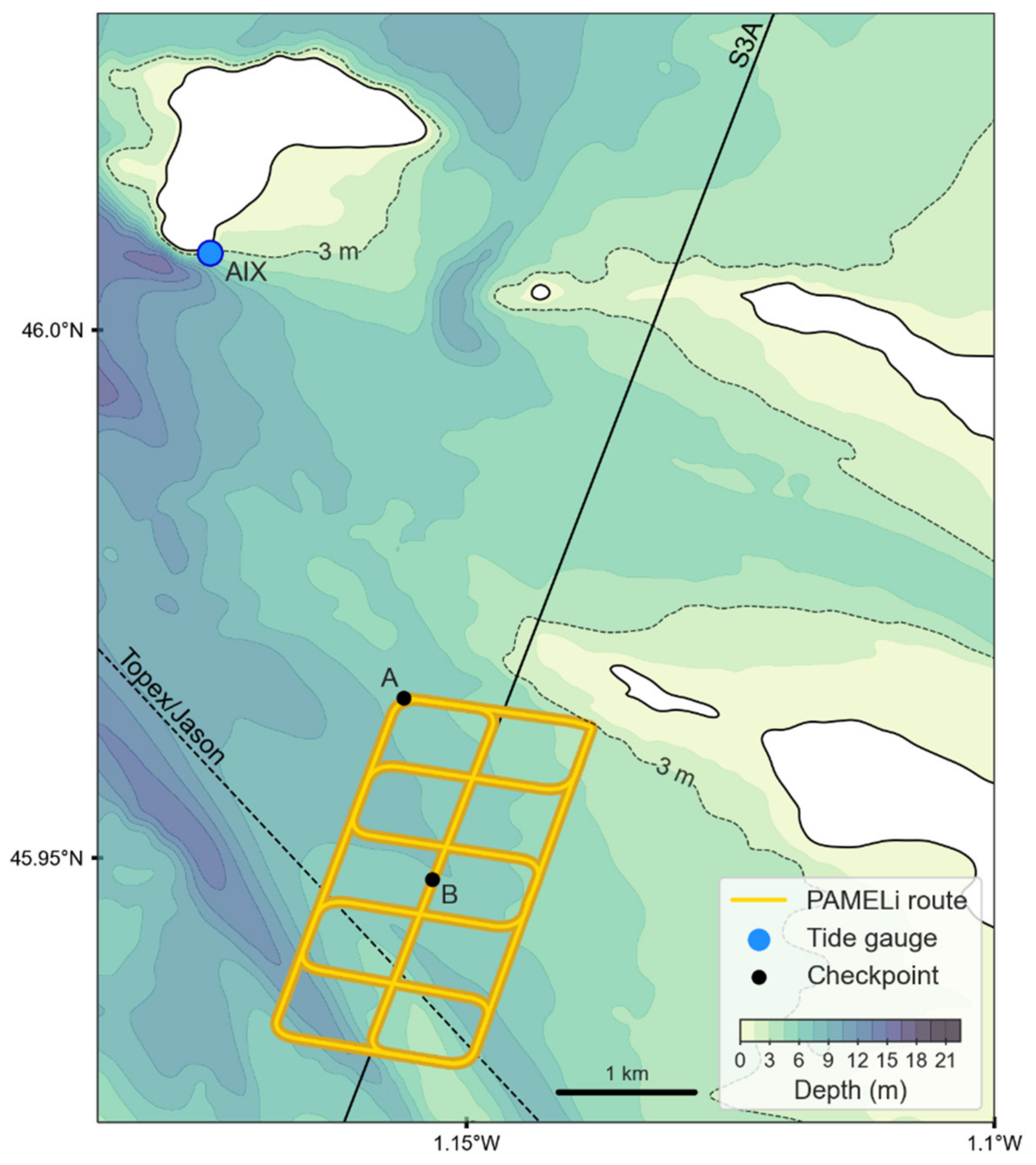
Two PAMELi surveys were performed between 29 and 30 July 2020. The USV main path consists of a route along Sentinel-3A track 216, identically repeated both days with self-intersecting segments. This gridded route is crisscrossed by four segments, separated by 750 m. The geometry configuration of the survey provides crossover measurements with a great variety of time intervals within each day (intra-day crossovers), in addition to the daily revisit between the two days of the survey (inter-day crossovers). Thanks to a precomputed GNSS route, the drone followed the exact same crossover itinerary both days at a constant speed of 3 knots by constantly adjusting its power engine amount. Despite an impact on the power consumption, the drone speed has proved to be very mildly affected by sea-state and wind conditions.
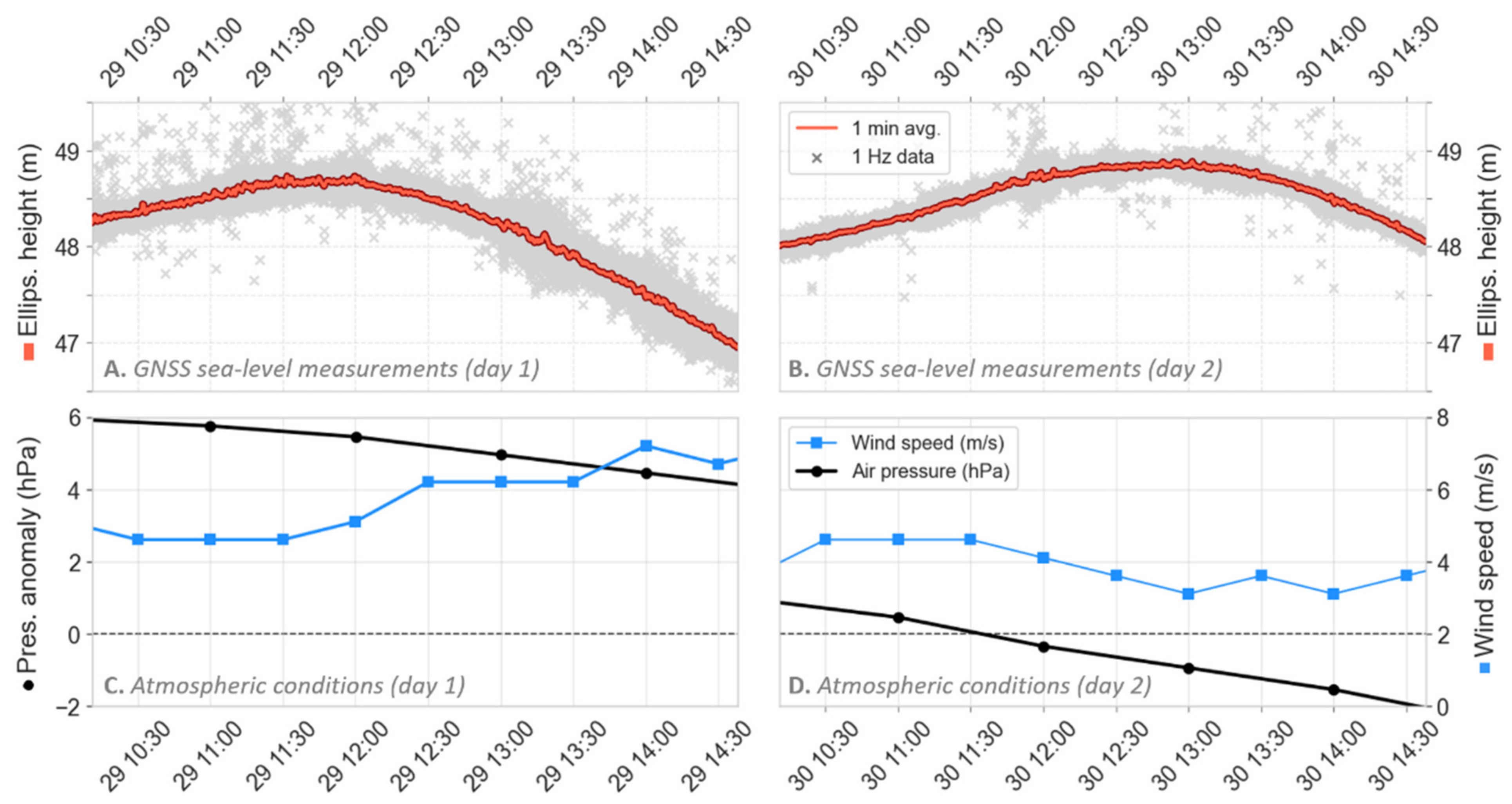
The cross-track distance (1.5 km) of the survey is large enough to cover the across track extent of Sentinel-3A passages, which can expand up to 750 m from the nominal track. The length of the survey is about 3.5 km along the Sentinel-3A track, with a maximal distance of 8.8 km from Aix Island permanent sea-level observatory. We started each survey day with a static session at AIX tide gauge to guarantee the GNSS processing before the start of the main survey. To save power consumption, PAMELi was towed to the starting point (point A in Figure 3) of the survey by the support boat at a constant speed of 6 knots. Then, the survey main route was completed by the drone between 10:10 and 14:40 on each day, constrained by logistical reasons. The 1Hz GNSS measurements from Cyclopée are post-processed with the RTKLIB software [27], using the double-difference method (detailed process in Supplementary Materials, Table S1). The AIX permanent GNSS station is used as a reference base throughout the survey. The baseline length being less than 10 km allows us to discard most of the tropospheric and ionospheric corrections (as well as the orbits and clocks uncertainties). The 1 Hz mean altimeter air-draft and the constant distance between instruments (GNSS and acoustic altimeter) are then subtracted from the GNSS heights to obtain the SSH observations along PAMELi tracks (Figure 4A,B). Finally, SSH measurements are averaged using a 1-min running window, in order to minor the impact of sea-state and GNSS noise on crossover differences (Figure 4A,B). Considering a constant speed of 3 knots during the survey, this 1-min filtering corresponds to a spatial averaging of roughly 300 m. The campaign was conducted during a moderate neap tide cycle associated to 4 m of tidal amplitude, with averaged winds increasing from 4 m·s−1 to 8 m·s−1 on the first day (Figure 4C) and decreasing from 5 m·s−1 to 3 m·s−1 on the second day (Figure 4D). The atmospheric pressure anomaly continuously decreases throughout the campaign from 6 hPa on the first day to −2 hPa on the second, which corresponds to a variation of −8 hPa during the two days of the campaign. Considering the linear inverse barometer assumption, this pressure drop corresponds to a sea-level height difference of roughly 8 cm that needs to be considered in the study.
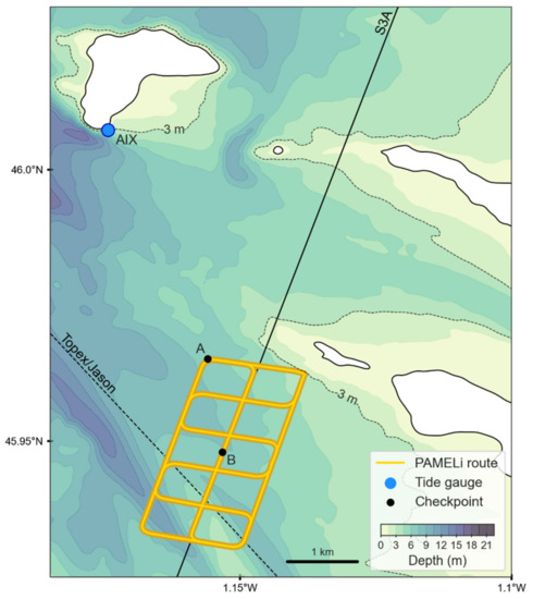
Figure 3.
PAMELi repeated survey during the two days campaign (yellow line). TP/Jason (dashed) and S3A (plain) nominal tracks are indicated by the grey straight lines. Aix island tide gauge (AIX) is represented by a blue circle. A and B black dots represent the starting point of the repeated survey and a reference point located at the middle of the survey extent, respectively. The grey contour is the 3 m isobath in the area.

Figure 4.
Cyclopée SSH measurements during the first (A) and second (B) day of the survey, for raw (1 s) (light grey crosses) and filtered (1 min) (red lines) measurements. These measurements are located at the same geographic position with a time interval of 24 h. Air pressure anomalies (black lines, left axis) and wind speed (blue lines, right axis) are displayed for the first (C) and second (D) day of the campaign (Météo-France data at Chassiron station on Oléron Island).
3.3. Crossover Methodology
The crossover method has been widely used in the early days of precise satellite altimeters to estimate and adjust the radial error of the spacecraft [22]. Since then, this methodology is currently used by the space agencies as a validation tool to assess the accuracy of the altimetry system (measurements and corrections). Following the approach used in [10,11], we propose in the present study an assessment of the residual heights at crossover points, after correcting the sea-level variation from our regional model. We can decompose the instantaneous ellipsoidal sea level as:
where is the ellipsoidal Mean Sea Level, is the Sea-Surface Height Anomaly, and represents the measurements errors, mostly due to instrumental or GNSS processing errors. For two co-located measurements at different times, we can thus determine the height difference :
Developing the sea-level terms from (1), this equation can be further decomposed in a relation where the stationary part (i.e., the MSL) is cancelled by the difference:
were represents the oceanic signal variation between time and (e.g., tides, atmospheric pressure effects, …) that can be estimated from hydrodynamic modelling. Then, after correcting the sea-level variation from the model, we define the crossover residuals as:
with the modeled sea-level difference between t and t + dt. reflects thus the ability of the model to accurately reproduce sea-level difference between two time-delayed measurements; a perfect correction would lead to a residual height containing only instrumental errors. Then, the objective is to use a combination of numerous crossover residuals () as a statistical indicator, for which the distribution can be analyzed to assess the accuracy of the model correction.
Crossover points are defined as a pair of co-located sea level measurements, separated by a time interval (dt). In the following, the term “crossover residual” refers to a residual height corrected from the model (), while “crossover difference” concerns the raw sea-level difference at a crossover point (). In this study, we used a maximum distance criterion of 50 m in order to minimize the influence of horizontal tidal and geoid gradients in crossover residuals. The crossover dataset includes pairs which are geometrical crossovers, but also measurements which are part of tracks that are close enough without necessarily crossing each other. Regarding the time separation criterion, crossover measurements with a time interval lower than 30 min are excluded from the selection in order to keep a residual significant in terms of tidal evolution, and to avoid a huge accumulation of successive measurements in the dataset. These criteria lead to a selection of 20,956 crossovers for the whole survey.
Considering the tidal signal as a summation of periodic waves, one must deal carefully with the time interval associated with crossover measurements, in order to consider the aliasing phenomenon in residuals. The contribution of a given tidal wave will not appear on a crossover difference if the time interval (dt) between the two measurements is similar to the wave period. Consequently, when assessing a tide correction, errors associated to this tidal wave will not be reflected in the residual height distribution. For instance, two measurements separated by dt = 12.42 h (or any multiple) would not reflect the contribution of M2, the major tide contribution in the region. On the other hand, the impact of a tidal wave in the residuals can be maximum for crossovers with a dt equal to the half of the wave period. However, its contribution depends not only on dt but also to the phase shift at the measurement times. In other words, the contribution of one tidal wave is minimized when the time interval corresponds to a phase shift of rad (or any multiple), whereas the maximum contribution can be reached when (but not necessary) the phase shift is rad. Thus, the survey has been designed to favor the representation of fourth-diurnal tidal waves contribution in crossover residuals (Figure S1—Supplementary Materials).
3.4. Model Setup
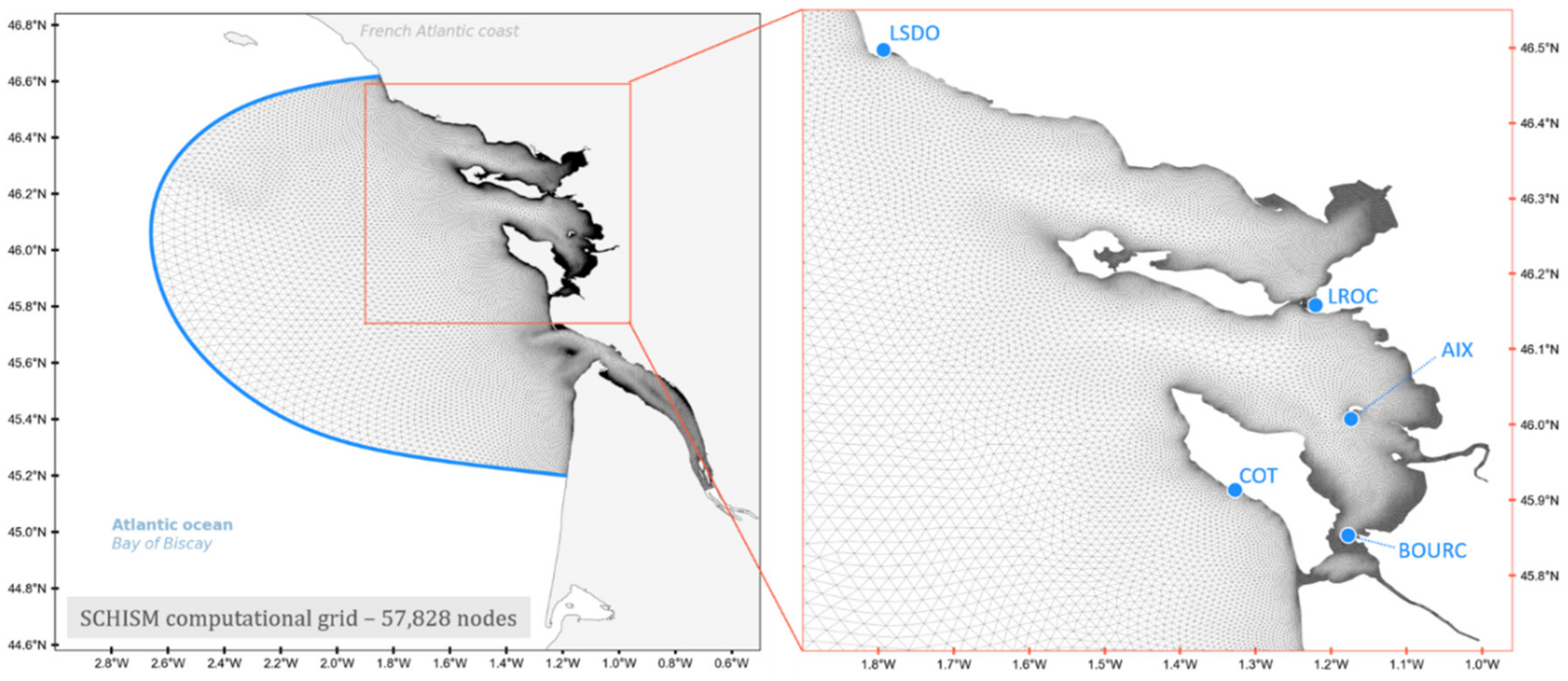
The numerical model used in this study is SCHISM (Semi-implicit Cross-scale Hydroscience Integrated System Model), a derivative product built from the original SELFE [28] with many enhancements and upgrades, including the seamless cross-scale capability from creek to ocean [14]. SCHISM is used here in depth-averaged barotropic mode, where vertically integrated shallow-water equations are solved on a finite-elements grid using Eulerian-Lagrangian (ELM) methods that guarantees high stability and efficiency. For the bathymetry, we use the HOMONIM dataset [29] provided by the French national hydrographic service (Shom). These dataset have a 20-m resolution in the Pertuis Charentais, and is composed of soundings completed by lidar surveys performed in the framework of the Litto3D project [30]. The model was forced over the whole domain by sea-level pressure and wind fields taken from the NCEP Climate Forecast System Reanalysis (CFSRv2) dataset [31]. The grid resolution varies from 3 km further on the shelf to 50 m in the shallower seas of the Pertuis Charentais, resulting in 57,828 nodes and 110,079 elements in total (Figure 5).

Figure 5.
Computational grid (57,828 nodes) used in the two model configurations. The left panel gives an overview of the grid extent over the continental shelf, within the Bay of Biscay, where the open boundary is indicated by the blue line. The right panel displays a close-up view of the Pertuis-Charentais area, with the 5 tide gauges used for model validation (blue labelled dots).
The tidal elevations are prescribed at the ocean boundary from a linear interpolation of the MAREST-NEA atlas, a state-of-the-art solution for the North-East Atlantic region (Shom/LEGOS) which benefits from an enhanced bathymetry developed in the framework of BathyCNES project (Noveltis/CNES) [32]. In detail, 4 of the 38 prescribed are taken from the assimilated solution developed by Noveltis in the framework of the BATHY CNES project (RegAT_NEAB_2019) [32]. The remaining constituents are derived from the hydrodynamic solution that the LEGOS team performed on the same configuration with drying/wetting tides and surges. A complete overview of the selected constituents and their numerical origin (hydrodynamic or assimilated) is proposed in the Supplementary Materials (Table S2).
In this study, we compare the correction from two SCHISM configurations which differ only by their tidal forcing:
- The first one (S) is the configuration described above, for which the tidal forcing are prescribed from the MAREST-NEA solution described above.
- For the second configuration (S+), we add empirical uniform biases in phases and amplitudes at the boundaries for M3 and MN4 constituents: +1.75 cm/−72° (M3) and +2.4 cm/+26° (MN4). These two constituents have a purely hydrodynamic numerical origin in the MAREST-NEA solution. The biases were determined through a careful regional comparison with tidal constituents derived from the Topex-Jason satellite altimetry (XTRACK product [33]) and tide gauges records [15,17] over the Bay of Biscay and the Pertuis-Charentais areas. An overview of this comparative study is shown in Figure S2—Supplementary Materials.
For both configurations, the tidal potential of the eight major constituents (M2, S2, K2, N2, K1, P1, O1, Q1) is applied over the whole domain, although it turned out to have a negligible impact on the simulations, given the limited size of the domain. The bottom friction is formulated through a constant Manning coefficient (n = 0.025) and a 240 s hydrodynamic time-step was selected after sensitivity tests. In the next section, we will assess these two configurations against coastal tide gauges and with the PAMELi crossover measurements methodology.
4. Results
4.1. Tide Gauge Validation
In order to assess the ability of the two model configurations to reproduce tide variability, amplitude and phase of modelled and observed sea-levels are computed for 13 constituents at 5 stations (LSDO, LROC, AIX, BOURC and COT, see Figure 5) using the python implementation of the harmonic analysis from UTide package software [34]. Astronomical and shallow-water constituents included in the analysis are referred to in Table 2.

Table 2.
Constituents included in the tide gauge validation.
For a given constituent, the complex difference is used to assess the tide error and computed as follows:
with the complex difference defined as:
where and are, respectively, the amplitude and the phase of observed (obs) and modelled (mod) tidal constituents. The combined complex error can thus be derived for a given site:
Finally, a global assessment can be given through the Root-Sum-Square (RSS), a combination of the error for all sites and waves:
For each station, the combined complex error of the 2 model configurations are displayed on Figure 6. The first configuration S exhibits good results (blue bars—Figure 6), with complex errors ranging from 4.32 cm (LSDO) to 8.23 cm (AIX station) and an RSS error of 6.24 cm for the 5 stations. By empirically correcting with uniform biases at the model boundary for M3 and MN4 waves, the S+ configuration reduces the errors at the 5 stations (green bars—Figure 6). While maximal site errors of 5.52 cm and 4.65 cm are reached at AIX and BOURC, they range between 2 cm and 3 cm at LSDO, LROC and COT tide gauges. The combination of these complex errors for the 5 stations gives an RSS of 3.83 cm, improving the RSS of the original solution by 2.41 cm.

Figure 6.
Combined complex errors of S (blue) and S+ (green) configurations, for 13 constituents at the 5 stations. The last bar chart (right, in bold) represents the Root-Sum-Square (RSS), combining all sites and all constituents.
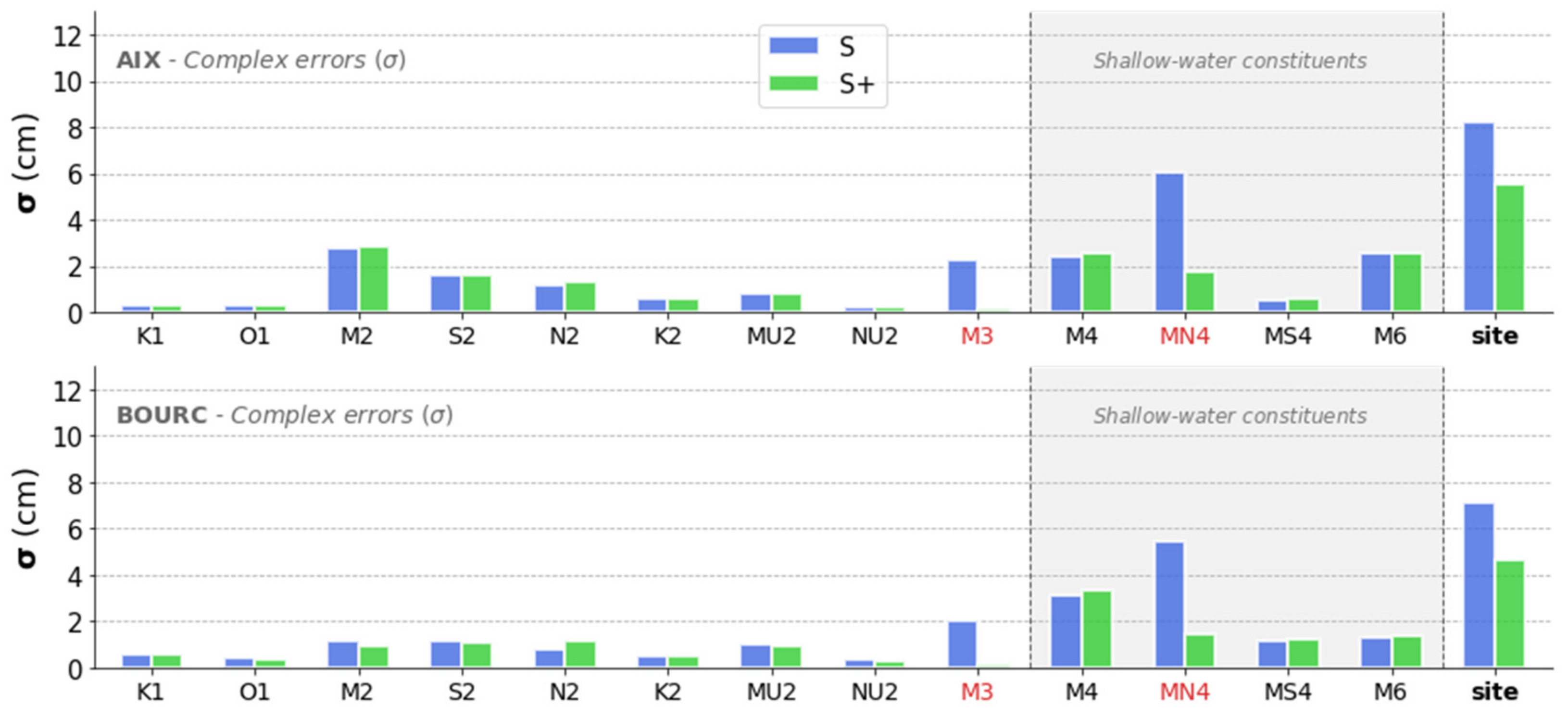
Tidal errors associated to each of the 13 constituents are detailed for AIX and BOURC tide gauges on Figure 7. These stations are particularly relevant since they are the closest to the survey (respectively at the north and the south). A complete overview of complex errors for the 5 stations is available in Supplementary Materials (Table S3). At AIX, the principal lunar constituent M2 and its non-linear overtides M4 and M6 are each associated with a 2–2.5 cm complex error. In proportion to their amplitude, it corresponds to roughly 1%, 8% and 50% of error. The shallow water waves constitute the main contribution to the total error budget, although the error is sensibly reduced in the case of MN4 when applying empirical biases (S+ configuration, green bars on Figure 7). At both sites, the 2 empirical biases on M3 and MN4 substantially improve the solution (Figure 7, last bar chart). While the remaining errors associated to M3 become marginal in S+, a significant error still remains on MN4, between 1.5 cm and 2 cm at BOURC and AIX.
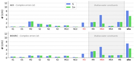
Figure 7.
Complex errors for the 13 major constituents at AIX (top panel) and BOURC (bottom panel) stations. For each constituent, errors associated to each configuration is represented: S (blue) and S+ (green). The last bar chart (right) represents the combined complex error for 13 constituents. Red labels correspond to constituents for which an empirical bias has been applied on the S+ forcing, and the bold right chart is the combined complex error for 13 constituents at the site.
It is noteworthy that complex errors associated to M2 and N2 slightly differ when corrections on M3 and MN4 are applied on S+. These sub-centimetric error differences are caused by a small amplitude reduction on M2 and N2 when applying the MN4 bias. It indicates that the main astronomical constituents are also marginally affected by non-linear interactions with the higher frequency waves they have generated.
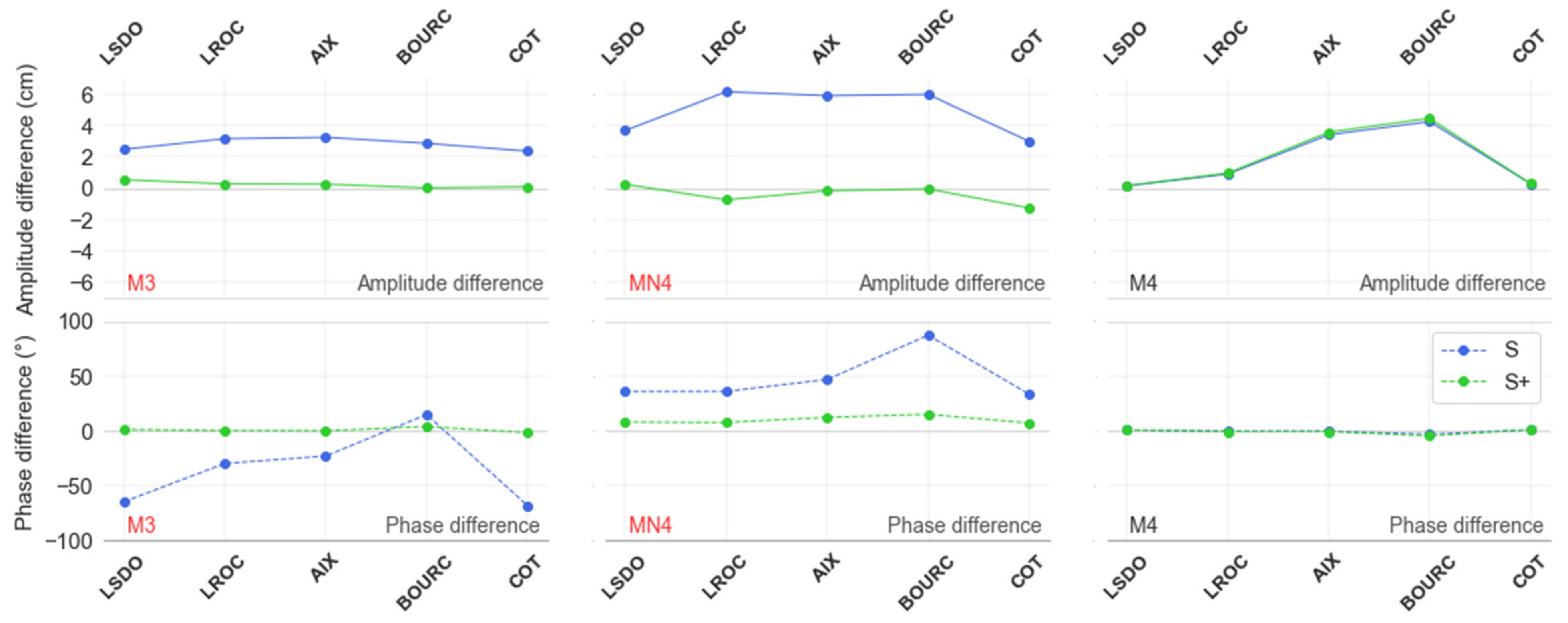
The Figure 8 shows the amplitude and phase differences between observations at the 5 tide gauges on both model configurations, for three constituents (M3, MN4 and M4). It is remarkable that the application at the open boundary of a spatially uniform bias on M3 phase and amplitude almost completely resolve the terdiurnal error for the 5 stations. While an important phase shift is observed with the original solution, ranging from −75° (COT) to 20° (BOURC), this terdiurnal tide is well phased at all stations with the improved configuration. It indicates the proper propagation of the M3 tide associated to the S+ configuration, and thus the validity of our empirical correction on M3 at the boundary. Concerning MN4, the phases and amplitudes better conform to the observations, although a phase shift remains at the 5 stations, reaching 18° at BOURC. As for the M3, we note that the phase shift is more homogeneous at the different stations with the S+ configuration. While the MN4 phase error ranges from 35° (LSDO) to 80° (BOURC) with the original forcing, it is in the range of 8° to 18° with the improved solution. While a 2.4 cm uniform bias is applied on the MN4 amplitude at the boundary, the gain is up to 6 cm at AIX and BOURC, reflecting the wave amplification throughout its propagation on the shelf and the Pertuis Charentais shallow waters.
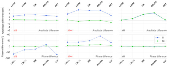
Figure 8.
Amplitude and phase differences between observed and modelled M3, MN4 and M4 at the 5 stations. Amplitude (top panel) and phase differences (bottom panel) at the 5 stations are computed for S (blue) and S+ (green) configurations. Red labels correspond to constituents for which an empirical bias has been applied on the S+ configuration.
Concerning M4, the large complex errors computed at AIX (2.2 cm) and BOURC (3 cm) stations are mostly due to an important bias in amplitude (Figure 8, right panel). While the phase shift is less than 5° for all stations, the amplitude is under-estimates by 4 cm at BOURC and 3.2 cm at AIX, for both configurations. It is noticeable that model and observations fit well at the two stations (LSDO, COT) located in the outer part of the Pertuis Charentais close to the open boundary (Figure 5). This also indicates that the amplitude error associated to M4 growths throughout its propagation inside the Pertuis Charentais sheltered seas, reflecting model discrepancies in its generation over these shallower waters.
In order to put these results in perspective with the performance of global models, we computed the same combined complex errors for the FES2014 solution [7] (Figure S3, Supplementary Materials). FES2014 is the latest version of the global Finite Element tidal Solutions series, but a new release is under development as part of the FES2022 project, which is expected to significantly improve the model coastal performances. The combined complex errors are significantly higher for FES2014 compared to S+ at all 5 stations (see Figure S3). It is interesting to note that, in regard to their amplitudes, shallow water constituents are the most improved with our regional configuration. Global models such as FES2014 are currently used for deriving SSHA from altimetry data, and these results show the importance of regional modelling for analysing coastal altimetry observations.
4.2. Crossover Differences and Residuals
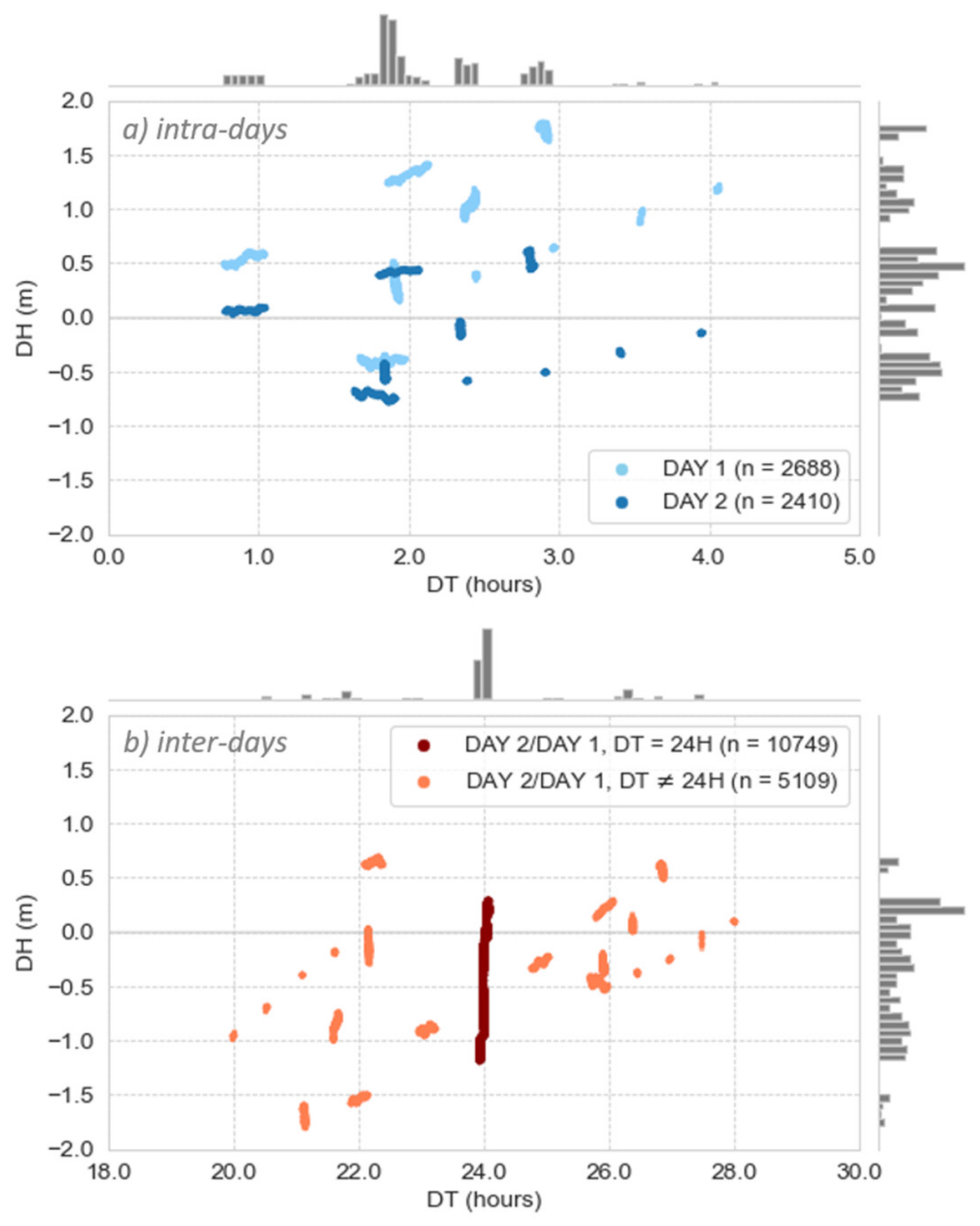
The criterion defined in Section 3.3 led to the computation of 2688 and 2410 crossover points within the first and second day. These intra-day differences (i.e., crossover points computed within a day) are associated with time intervals ranging from 1 h to 4 h. The 2, 2.5 and 3 h intervals are the most represented, which is, in theory, favourable to highlight the contribution of 4th and 6th diurnal tidal waves in the residuals distribution. Crossover differences (DH) associated to these intra-day crossovers are reasonably spread, ranging from −0.8 m to 1.8 m (Figure 9a).
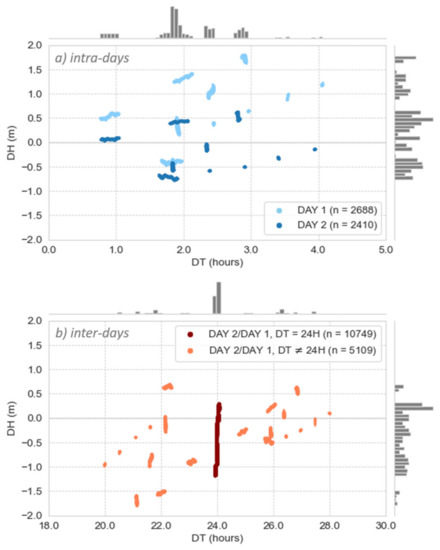
Figure 9.
Representation of intra-day (a) and inter-day (b) crossover differences (DH) in function of the time interval dt. For each panel, top and right grey histograms, respectively, represent the temporal and height distributions of crossovers.
Regarding the inter-day crossovers (i.e., crossover points associated with height measurements from two successive days), the repeat survey led to the computation of 15,858 crossover differences, associated to time intervals ranging from 20 to 28 h (Figure 9b). The inter-day crossover differences (DH) range from −1.8 m to 0.8 m with a notable peak around the 0.25 m difference. Because of the scheduled planning of the campaign, most of these differences are associated with a time interval of exactly 24 h (68% of the total number of inter-day crossovers). Since the 24 h time interval aliases the main solar astronomical constituent S2 and its shallow water overtide S4, their contributions do not appear in the differences associated to this time interval. Moreover, this time interval is also close to the period of the major semi-diurnal constituents, which minors their contribution in crossover differences.
These crossover differences are then corrected from the modelled sea-level variations following the Equation (4) of Section 3.3. This correction is obtained by linearly interpolating the modelled SLA at exact times and locations of crossover measurements. It accounts for the tide and atmospheric dynamics that are modelled in our configurations. We thus obtain crossover residuals (DHRES) that reflect the ability of our barotropic model to correct the sea-level variations during the survey. The density distributions of crossover residuals are computed for intra-day (Figure 10) and inter-day (Figure 11) for both model configurations (S—blue, S+—green).

Figure 10.
Density distribution of intra-day crossover residuals (DHRES) for the 2 model configurations: S (blue) and S+ (green). Residuals from day 1 and day 2 are shown, respectively, on left and right panels.

Figure 11.
Density distribution of inter-day crossover residuals (DHRES) for the 2 different configurations: S (blue) and S+ (green). The left panel distribution corresponds to crossover residuals associated to a 24 h return period, and the right panel displays the leftovers.
As for the tide gauge validation results, our modified configuration (S+) significantly reduces the residuals at crossover measurements. For the intra-day residuals (Figure 10), the RMSE is reduced from 11.66 cm to 4.2 cm (Day 1, left panel) and from 12.7 cm to 4.1 cm (Day 2, right panel) in comparison to the original solution (S). Thus, applying the empirical tidal forcing correction for M3 and MN4 reduces by roughly 60% the error associated to the intra-day crossovers. It is reflected by the distribution shapes, which become purely unimodal with a mean residual height of, respectively, −2.34 cm and −3.52 cm on the first and second day. With the original correction (S), the residuals distribution is flatter and less symmetrical, with a mean residual of −10 cm for both days.
For the inter-day residuals, crossovers associated with a 24 h time interval are considered apart (Figure 11, left panel) than the others that range from 20 h to 28 h (Figure 11, right panel). It is justified by the fact that these crossovers are the most represented due to the survey design and are less likely to highlight tidal errors in the residual heights. For this reason, crossover residuals associated with the 24 h time interval are the least spread and biased from our dataset, with a RMSE of 5.65 cm for the original solution (S) against 3.02 cm for the improved solution (S+) (Figure 11, left panel). The gain for S+ here is moderate in comparison to the other crossover residuals (intra-days and inter-days with dt ), confirming that a time interval of 24 h between two measurements minors the mismodelling contribution of the third and fourth diurnal. The residual distribution of the remaining inter-day crossovers (dt ), with time intervals ranging from 20 h to 28 h, is shown on the right panel of Figure 11. As for intra-day crossovers, the dispersion of these residuals is reduced by 60% when correcting with S+ compared to the original solution S (RMSE = 4.04 cm against 11.73 cm). The particularity of the distribution for S+ residuals is a remaining bimodal shape, while it is only unimodal (but biased) for intra-day crossovers. This can be explained by the fact that for these inter-day crossovers, time intervals range from 20 h to 28 h, which allow to completely browse the period of the third and fourth diurnal tidal cycles. This bimodal shape is still visible in the distribution corrected by S+ (green curve, Figure 11, right panel), although the residual heights are less dispersed (RMSE = 4.04 cm for S+ against 11.73 cm for S).
In order to statistically quantify the improvements made by applying empirical biases for M3 and MN4 at boundary forcing, we calculate the percentile distribution for S and S+ corrections (Figure 12). This indicator represents the percentage of residuals below a given value. For instance, the 50th percentile represent the maximum height residual reached by 50% of the crossovers (i.e., the median). In addition to the median, we compute the 90th percentile which excludes the largest 10% of crossover residuals, thus putting aside outliers (which can reflect instrumental errors). All the crossover residuals corrected from our improved solution (S+) are lower than 10 cm. The 90th percentile is 5.81 cm, while 50% of the residuals are below 2.5 cm (i.e., the median). When corrected with the original configuration (S), the percentiles are roughly three times higher, with a 90th percentile of 15.22 cm and a median of 7.33 cm.

Figure 12.
nth percentiles distribution of the crossover residuals, for the S (blue) and S+ (green) corrections. The 50th and 90th percentiles are represented by vertical lines, and associated values are displayed for each configuration.
5. Discussion and Perspectives
5.1. Importance of Survey Design: The MN4 Example
In the following section, we further investigate the independent contribution of MN4 to better understand the crossover improvements in terms of survey design. For this purpose, we used the harmonic prediction formula defined as follow:
where , and are the amplitude, the phase lag, and the angular speed of the constituent , and the time of the prediction. and are the nodal modulation amplitude and phase correction factors, while is the astronomical argument at initial epoch [35]. At a given time, the contribution of one tidal wave k to the sea-level is determined from (8):
The Equation (2) can thus be applied between the reconstructed tidal height at times t and t + dt, to give the contribution of the wave to crossover differences:
in order to interpret the contribution of a given constituent in the light of its tidal phase, the corresponding crossover phase shifts () are computed as follows:
where is the time interval associated to a pair of measurements, and is the tidal period for constituent k. In other words, links a crossover time interval and the state of evolution of a constituent and is in the range in the , allowing us to represent the time interval (dt) in the periodic interval.
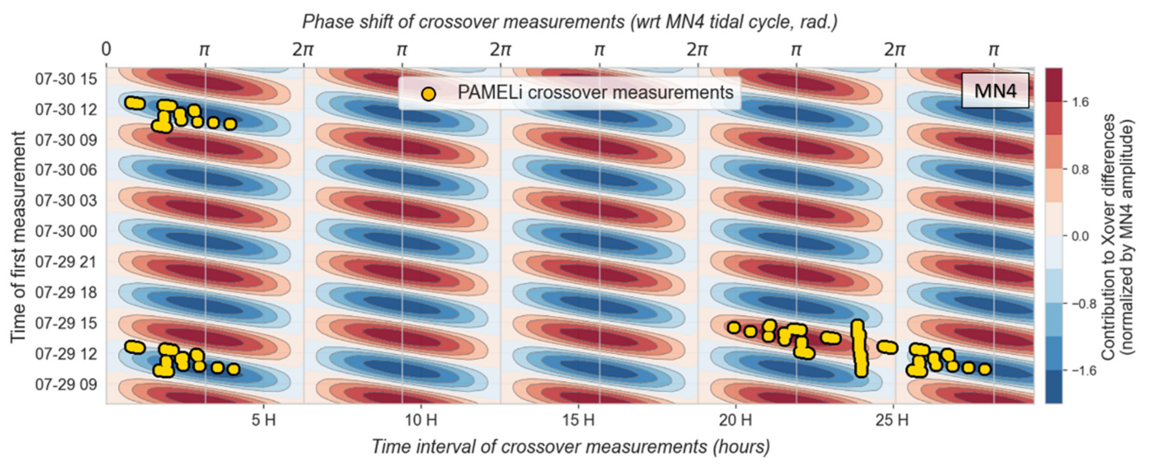
Based on amplitudes and phases at AIX, the MN4 contribution to crossover differences is computed following (10) and normalized by its amplitude (Figure 13). The concentric ellipses represent the contribution in crossover difference heights, which reach an absolute maximum of two-times the amplitude on their centres. While these height differences can thus be negative (blue) or positive (red), white areas represent the time/phase shift associations for which the two MN4 heights are similar and vanish in the difference. The crossover points collected during our two-day campaign are represented on the same layout (Figure 13, yellow dots), showing the survey design from the point of view of the MN4 tidal cycle at AIX. The inter-day crossovers browse a complete fourth-diurnal cycle, with negative and positive MN4 contributions to the crossover distribution (Figure 13, dt between 18 and 28 h). It explains why the residuals have a bimodal distribution for the inter-day crossovers (Figure 11, right panel) with the original model correction, considerably attenuated when correcting with S+. On the contrary, time intervals of intra-day crossovers are not sufficiently spread to browse a complete fourth-diurnal cycle (Figure 13, dt lower than 5 h), and the S residual distributions are thus unipolarly biased (Figure 10). The negative bias in the distribution is almost resolved with the S+ correction, which reproduces more accurately MN4, as shown before.
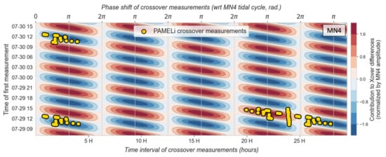
Figure 13.
Contribution of MN4 to crossover differences (), normalized by its amplitude. The PAMELi crossover measurements (yellow dots) are displayed with respect to their crossover time-intervals (bottom x-axis) and the corresponding phase shifts (top x-axis). The y-axis represents the time of crossover first measurements.
The survey temporal design, that is the phase shift of a pair of measurements, is thus a crucial parameter that determines the contribution of a tidal wave in crossover residuals. For a given tidal wave, some time-intervals (corresponding to a specific phase shift of the wave) are more favourable to highlight the contribution of the wave in a crossover difference. Reciprocally, the pertinence of this methodology highly depends on this latter parameter, which has to be considered in the preparation of the survey. For this purpose, a planification tool is currently being developed to help in the preparation of future validation campaigns. For this study, we used a tide prediction computed at AIX station to have an a-priori knowledge of tidal cycles and thus optimize the crossover measurements for fourth-diurnal waves, as the shallow-water wave MN4 which is strongly amplified throughout its propagation on the shelf. By applying a bias of +2.4 cm on the open boundary, the amplitude difference between our two configurations reach +8 cm at the survey location. In our collection of crossovers, this bias of +8 cm is thus reflected by differences reaching 16 cm (two times the amplitude difference) in crossover residuals, when measurements are separated by a phase shift of rad.
After reducing the error on M3 and MN4 with the S+ configuration, the major contribution in the fourth-diurnal error budget for S+ is now the M4 wave (Figure 7), for which the impact on crossover residuals is discussed in the next section.
5.2. Error Budget Associated to M4
From tide gauges validation results (Section 4.1), it appears that a large error remains on the M4 tidal wave with the S+ configuration. While this fourth-diurnal wave is well reproduced on the outer part of the Pertuis Charentais area (0.2 cm and 0.3 cm of complex errors at LSDO and COT), mismodeling appear throughout its propagation toward shallower seas (2.5 cm and 3.3 cm of c.e. at AIX and BOURC, see Figure 7 and Table S3—Supplementary Materials). Since the survey took place between AIX and BOURC stations), a significant impact of the M4 error on our crossover residuals are expected. In order to quantify the impact of the M4 amplitude mismodelling error in crossover residuals, we introduce a correction term based on the tide prediction formula (10), defined as follows:
where is the M4 amplitude error that has to be determined, and the phase lag computed from model at the centre of the survey (B point in Figure 3). The corrected sea-level at a given time can thus be determined as:
and the corrected crossover residual is computed as previously, accounting for this corrected term, by subtracting the corrected SSH at both measurement times:
In other words, we compare our best model correction (S+) with a new solution which account for an empirical M4 correction term, at the survey location. Hereafter, we discuss the impact of this correction term on the crossover residuals distributions. The amplitude bias apply for M4 is = 2.3 cm. The latter has been determined through a sensibility study, minimizing the residual heights. These corrected distributions of intra-day and inter-day residuals are displayed on Figure 14. Crossovers associated to a 24 h revisit time are not included in the analysis here because they reflect less the contribution of quarter-diurnal waves and are thus less impacted by this correction term. Furthermore, the 24 h time interval being the most sampled (50% of the total number of crossovers), its inclusion in the statistical indicators would partially dampen the impact of the corrected term. For the two intra-day distributions (day 1 and day 2) (Figure 14a,b), the M4 correction substantially improves the residual errors. The mean residual decreases from −2.34 cm to 0.22 cm for the first day and from −3.52 cm to −1.4 cm for the second day. RMSE associated with these two days is also improved by 0.62 cm and 1.12 cm, respectively. For the inter-day crossover distribution (Figure 14c), the RMSE is improved by 0.79 cm, from 4.04 cm to 3.25 cm. For these crossovers, the shape of the distribution is much more unimodal with this M4 correction, reflecting a more accurate reproduction of sea-level variations within the whole tidal cycle.

Figure 14.
Crossover residuals density distributions for S+ (green) and S+ empirically corrected from M4 amplitude error (dashed black line). The root-mean-square errors (RMSE) and the mean are represented for each configuration, in the corresponding colour. Only distributions associated to intra-day ((a) day 1, (b) day 2) and inter-day with time interval different from 24 h (c) are shown.
As presented in the result section, we compute the percentiles distribution of the corrected solution (Figure 15), which is computed for all crossover residuals, except for those associated with dt = 24 h (in contrast to the percentiles showed in Figure 12, computed for all crossover residuals). Percentiles are computed from absolute crossover residual values corrected for the two latter configurations. The M4 correction term improves the global accuracy, by roughly 1 cm for all percentiles higher than the 20th. Thus, the 50th (median) and the 90th centiles are improved from 3.19 cm to 2.1 cm and from 6.37 cm to 5.56 cm, respectively. In other words, 50% of crossover corrected residuals are below 2.1 cm with this solution.

Figure 15.
nth percentiles distribution of the crossover residuals, for S+ (green) and S+ empirically corrected from M4 amplitude error (dashed black line). The 50th and 90th centiles are represented by vertical lines, and associated values are displayed for each configuration. Percentiles are computed for absolute values of crossover residuals issued from intra-day and inter-day (excluding the 24 h time intervals).
By providing spatially extended validation capabilities, this methodology based on USV can thus be very useful to fine-tune the model, in particular for the bottom drag parametrization. Numerous studies have shown the importance of bottom drag in the quarter and sexta-diurnal generation mechanisms [8,25,36]. For instance, Song et al. showed that 36% of M4 was generated by the frictional momentum in the Baya Bay, China. The bottom friction parametrization is not addressed in the presented study and a constant manning coefficient (n = 0.025) is applied over the whole domain. However, the bottom friction coefficient depends on the seabed nature, and its variation can have a strong impact on the tidal amplitudes [20,36]. The presence of large intertidal mud flat areas on both sides of the Marennes-Oléron bay, where this validation study takes place, tends to locally reduce the friction, and enhance the tidal propagation. In this area, Nicolle et al. [25] showed that a simple two-zone parameterization of the bottom drag coefficient leads to a better reproduction of the propagation of shallow water waves.
A further study including a more appropriate parametrization should lead to better reproduction of the shallow water tide, including M4 and M6, for which significative errors are present with our model configuration. Such improvements would significantly improve the agreement at crossover points where shallow-water waves constitute a major part of the error budget.
6. Conclusions
In this study, we propose an original application of the use of new sea-level mapping tools in combination with a crossover methodology to assess the performances of two hydrodynamic models developed for the Pertuis Charentais area. Both configurations are forced with tidal elevations from a state-of-the-art regional atlas, and we applied empirical uniform biases in phases and amplitudes at the boundaries for M3 and MN4 on the second configuration. After a classic tide gauge validation, we assess the accuracy of the two model configurations under a Sentinel-3A track by performing a crossover analysis on sea-level data collected in July 2020, using PAMELi, an USV developed at La Rochelle University and equipped with the Cyclopée system (a combination of a GNSS antenna and an acoustic altimeter). The second model configuration improves the Root-Mean-Square Error (RMSE) by 20–30% at tide gauges located in the inner part of the Pertuis Charentais and reduces the RMSE by more than 60% for the survey crossover residuals, under the Sentinel-3A track. We show that the survey design is essential to emphasize the contribution of third-diurnal and fourth-diurnal waves in the crossover residual distributions. For instance, the bias of +2.4 cm applied over the boundary for MN4 leads to an amplitude difference of +8 cm between the two configurations at the survey location, which is reflected by differences up to 16 cm in crossover residuals. We also use crossover residual heights to investigate the impact of M4 amplitude errors, by introducing an empirical correction term based on M4 observations at tide gauges. Adding this correction further reduces the RMSE of crossover residuals by 15–25%.
This study is a proof of concept which demonstrates the potential of using the innovative USV platforms to spatially-extend model validation capabilities. We use these new sea-level observations by computing crossovers time-differences to assess model performances. Through an analysis of two model configurations, the survey design turned out to be a determining factor given the periodic nature of tide observations. Further tests must be carried out to improve the methodology, such as repeating this study over larger areas where the tidal and geoid gradients become more significant. This will be crucial in the scope of the future SWOT mission, for which the accuracy of tide correction must be assessed over the large-extent areas covered by swaths observations. Since very few applications involving USVs in ocean modelling have been reported, we hope that this study will stimulate further investigations in this field.
Supplementary Materials
The following are available online at https://www.mdpi.com/article/10.3390/rs13152886/s1, Table S1: RTKLib differential GNSS processing parameters used in this study, Figure S1: Superimposition of pairs of intra-day crossovers with the theoretical residuals computed from a tide reconstruction at Aix Island station, for M2 (left), M4 (middle) and M6 (right). The residual height is normalized by its maximum, within each frequency band. Crossovers measurements of day 1 (light blue dots) and day 2 (deep blue dots) are graphically represented with their initial time and the time interval with the second measurements (dt) as coordinates, Table S2: Prescribed constituents for tidal elevation at model boundary. The 4 dotted constituents are derived from the assimilated solution of Noveltis (BATHY CNES, RegAT_NEAB_2019). Red labels correspond to the two constituents for which an empirical bias has been applied on the S+ forcing, Figure S2: Amplitude and phase differences between observations and MAREST-NEA atlas over the Bay of Biscay, for M3 (top panel) and MN4 (bottom panel). Observations are derived from Topex-Jason satellite altimetry (XTRACK product and tide gauges records), Table S3: Complex errors computed at the 5 stations used in model validation for the two model configurations, Figure S3: Complex errors for the 13 major constituents at AIX (top panel) and BOURC (bottom panel) stations. For each constituent, errors associated to each configuration is represented: FES2014 (grey), S (blue), S+ (green). The last bar chart (right) represents the combined complex error for 13 constituents. Red labels correspond to constituents for which an empirical bias has been applied on the S+ forcing.
Author Contributions
Y.-T.T., L.T., C.C. and V.B. designed the study, Y.-T.T., L.T., C.C. and V.B. designed and conducted the field campaign, C.C. processed the GNSS data, Y.-T.T. processed the data and wrote the original draft of the paper. Writing—review & editing, L.T., C.C., V.B. and P.B. All authors have read and agreed to the published version of the manuscript.
Funding
This study has been conducted and financed thanks to the Centre National d’Etudes Spatiales (CNES), through the TOSCA FOAM project, the Centre National de la Recherche Scientifique (CNRS) and French Ministry of Research. Funding for Y.-T.T. is provided by the French Ministry of Research, while C.C. is funded by the Direction Générale de l’Armement (DGA) and the Nouvelle Aquitaine region. The USV PAMELi used in this study has been funded by the Region Nouvelle Aquitaine through the CPER RISCO and the Cyclopée system has been designed by DT INSU.
Institutional Review Board Statement
Not applicable.
Informed Consent Statement
Not applicable.
Data Availability Statement
X-TRACK Tidal Constants (amplitudes, phase lags and associated estimation errors for 73 constituents) derived from the X-TRACK T/P and Jason 1&2 used for model tuning are produced by CTOH and distributed on AVISO+ website: https://www.aviso.altimetry.fr/en/data/products/auxiliary-products/coastal-tide-xtrack.html. REFMAR tide gauge records used for model validation can be retrieved from the SHOM web portal: https://data.shom.fr. Both web pages have been accessed on 21 July 2021. GNSS and sea-level data produced during the USV survey will be gladly provided upon a request to the corresponding author at: yanntreden.tranchant1@univ-lr.fr.
Acknowledgments
The authors want to thank Thibault Coulombier and Denis Dausse for the preparation of the PAMELi survey and the technical support and Yves Bryzard, the boat pilot during the July 2020 mission. We also thank Florent Lyard (Legos) and Mathilde Cancet (Noveltis) for providing regional tidal boundary forcing, developed in the framework of BathyCNES project (Noveltis/CNES). Tidal constituents computed for the bottom pressure data collected during TRANSEPLAT (1983) and CIRESOL (1987) campaigns were kindly provided by Bertrand Le Cann.
Conflicts of Interest
The authors declare no conflict of interest. The funders had no role in the design of the study; in the collection, analyses, or interpretation of data; in the writing of the manuscript, or in the decision to publish the results.
References
- Fu, L.-L.; Alsdorf, D.; Morrow, R.; Rodriguez, E.; Mognard, N. SWOT: The Surface Water and Ocean Topography Mission: Wide-Swath Altimetric Elevation on Earth; Jet Propulsion Laboratory, National Aeronautics and Space Administration: Pasadena, CA, USA, 2012.
- Morrow, R.; Fu, L.-L.; Ardhuin, F.; Benkiran, M.; Chapron, B.; Cosme, E.; d’Ovidio, F.; Farrar, J.T.; Gille, S.T.; Lapeyre, G.; et al. Global Observations of Fine-Scale Ocean Surface Topography With the Surface Water and Ocean Topography (SWOT) Mission. Front. Mar. Sci. 2019, 6. [Google Scholar] [CrossRef]
- Stammer, D.; Cazenave, A. Satellite Altimetry Over Oceans and Land Surfaces; CRC Press: Boca Raton, FL, USA, 2017; ISBN 978-1-4987-4346-4. [Google Scholar]
- Bonnefond, P.; Verron, J.; Aublanc, J.; Babu, K.N.; Bergé-Nguyen, M.; Cancet, M.; Chaudhary, A.; Crétaux, J.-F.; Frappart, F.; Haines, B.J.; et al. The Benefits of the Ka-Band as Evidenced from the SARAL/AltiKa Altimetric Mission: Quality Assessment and Unique Characteristics of AltiKa Data. Remote Sens. 2018, 10, 83. [Google Scholar] [CrossRef] [Green Version]
- Peng, F.; Deng, X. Validation of Sentinel-3A SAR Mode Sea Level Anomalies around the Australian Coastal Region. Remote Sens. Environ. 2020, 237, 111548. [Google Scholar] [CrossRef]
- Laignel, B.; Ayoub, N.; Birol, F.; Brown, S.; Chao, Y.; Cornuelle, B.; Costa, S.; de Mey, P.; Estournel, C.; Feddersen, F.; et al. Issues and SWOT Contribution in the Coastal Zones and Estuaries White Paper; SWOT White Papers; NASA: Washington, DC, USA, 2015.
- Lyard, F.H.; Allain, D.J.; Cancet, M.; Carrère, L.; Picot, N. FES2014 Global Ocean Tide Atlas: Design and Performance. Ocean Sci. 2021, 17, 615–649. [Google Scholar] [CrossRef]
- Le Provost, C. Generation of overtides and coupound tides (review). In Tidal Hydrodynamics; Parker, B.B., Ed.; John Wiley & Sons: Hoboken, NJ, USA, 1991; pp. 269–289. ISBN 978-0-471-51498-5. [Google Scholar]
- Ayoub, N.; Birol, F.; Brown, S.T.; Chao, Y.; Cornuelle, B.; de Mey, P.; Estournel, C.; Giddings, S.; Gille, S.; Kurapov, A.; et al. Coastal and Estuaries White Paper. Part 2: Coastal Seas and Shelf Processes; SWOT White Papers; NASA: Washington, DC, USA, 2017.
- Bonnefond, P.; Exertier, P.; Laurain, O.; Ménard, Y.; Orsoni, A.; Jeansou, E.; Haines, B.J.; Kubitschek, D.G.; Born, G. Leveling the Sea Surface Using a GPS-Catamaran Special Issue: Jason-1 Calibration/Validation. Mar. Geod. 2003, 26, 319–334. [Google Scholar] [CrossRef]
- Bonnefond, P.; Laurain, O.; Exertier, P.; Calzas, M.; Guinle, T.; Picot, N. Validating a New GNSS-Based Sea Level Instrument (CalNaGeo) at Senetosa Cape. Mar. Geod. 2021. under review. [Google Scholar]
- Brachet, C.; Calzas, M.; Drezen, C.; Fichen, L.; Guillot, A.; Téchiné, P.; Testut, L.; Bonnefond, P.; Laurain, O.; Umr, G.; et al. Mesure du Geoïde Marin Avec le Système CalNaGEO (GNSS). 2019. Available online: http://www.legos.obs-mip.fr/observations/rosame/documents/CalNaGEO_Refmar_2019.pdf (accessed on 21 July 2021).
- Chupin, C.; Ballu, V.; Testut, L.; Tranchant, Y.-T.; Calzas, M.; Poirier, E.; Coulombier, T.; Laurain, O.; Bonnefond, P.; Team FOAM Project. Mapping Sea Surface Height Using New Concepts of Kinematic GNSS Instruments. Remote Sens. 2020, 12, 2656. [Google Scholar] [CrossRef]
- Zhang, Y.J.; Ye, F.; Stanev, E.V.; Grashorn, S. Seamless Cross-Scale Modeling with SCHISM. Ocean Model. 2016, 102, 64–81. [Google Scholar] [CrossRef] [Green Version]
- Pouvreau, N. REFMAR: Une coordination pour l’observation du niveau de la mer. Houille Blanche 2014, 37–43. [Google Scholar] [CrossRef]
- André, G.; Míguez, B.M.; Ballu, V.; Testut, L.; Wöppelmann, G. Measuring Sea Level with GPS-Equipped Buoys: A Multi-Instruments Experiment at Aix Island. Int. Hydrogr. Rev. 2013. Available online: hwww.psmsl.org/about_us/news/2013/workshop_2013/posters/Poster_GPSbuoys_multipurpose.pdf (accessed on 21 July 2021).
- Le Cann, B. Barotropic Tidal Dynamics of the Bay of Biscay Shelf: Observations, Numerical Modelling and Physical Interpretation. Cont. Shelf Res. 1990, 10, 723–758. [Google Scholar] [CrossRef]
- Bertin, X.; Bruneau, N.; Breilh, J.-F.; Fortunato, A.B.; Karpytchev, M. Importance of Wave Age and Resonance in Storm Surges: The Case Xynthia, Bay of Biscay. Ocean Model. 2012, 42, 16–30. [Google Scholar] [CrossRef]
- Dodet, G.; Bertin, X.; Bouchette, F.; Gravelle, M.; Testut, L.; Wöppelmann, G. Characterization of Sea-Level Variations Along the Metropolitan Coasts of France: Waves, Tides, Storm Surges and Long-Term Changes. J. Coast. Res. 2019, 88, 10. [Google Scholar] [CrossRef]
- Pairaud, I.L.; Lyard, F.; Auclair, F.; Letellier, T.; Marsaleix, P. Dynamics of the Semi-Diurnal and Quarter-Diurnal Internal Tides in the Bay of Biscay. Part 1: Barotropic Tides. Cont. Shelf Res. 2008, 28, 1294–1315. [Google Scholar] [CrossRef]
- Clarke, A.J.; Battisti, D.S. The Effect of Continental Shelves on Tides. Deep Sea Res. Part Oceanogr. Res. Pap. 1981, 28, 665–682. [Google Scholar] [CrossRef]
- Ray, R.D. First Global Observations of Third-Degree Ocean Tides. Sci. Adv. 2020, 6, eabd4744. [Google Scholar] [CrossRef]
- Huthnance, J.M. On Shelf-Sea ‘Resonance’ with Application to Brazilian M3 Tides. Deep Sea Res. Part Oceanogr. Res. Pap. 1980, 27, 347–366. [Google Scholar] [CrossRef]
- Nicolle, A.; Karpytchev, M.; Benoit, M. Amplification of the Storm Surges in Shallow Waters of the Pertuis Charentais (Bay of Biscay, France). Ocean Dyn. 2009, 59, 921–935. [Google Scholar] [CrossRef]
- Nicolle, A.; Karpytchev, M. Evidence for Spatially Variable Friction from Tidal Amplification and Asymmetry in the Pertuis Breton (France). Cont. Shelf Res. 2007, 27, 2346–2356. [Google Scholar] [CrossRef]
- Coulombier, T.; Ballu, V.; Pineau, P.; Lachaussee, N.; Poirier, E.; Guillot, A.; Calzas, M.; Drezen, C.; Fichen, L.; Plumejeaud, C.; et al. PAMELi, un drone marin de surface au service de l’interdisciplinarité. In Proceedings of the XVèmes Journées Nationales Génie Côtier-Génie Civil, La Rochelle, France, 29–31 May 2018; pp. 337–344. [Google Scholar]
- Takasu, T.; Yasuda, A. Development of the Low-Cost RTK-GPS Receiver with an Open Source Program Package RTKLIB; International Convention Center: Jeju, Korea, 2009. [Google Scholar]
- Zhang, Y.; Baptista, A.M. SELFE: A Semi-Implicit Eulerian–Lagrangian Finite-Element Model for Cross-Scale Ocean Circulation. Ocean Model. 2008, 21, 71–96. [Google Scholar] [CrossRef]
- MNT. Topo-Bathymétrique Côtier des Pertuis Charentais (Projet Homonim); SHOM: Brest, France, 2015. [Google Scholar] [CrossRef]
- Louvart, L.; Grateau, C. The Litto3D Project. In Proceedings of the Europe Oceans 2005, Brest, France, 20–23 June 2005; Volume 2, pp. 1244–1251. [Google Scholar] [CrossRef]
- Saha, S.; Moorthi, S.; Wu, X.; Wang, J.; Nadiga, S.; Tripp, P.; Behringer, D.; Hou, Y.-T.; Chuang, H.; Iredell, M.; et al. NCEP Climate Forecast System Version 2 (CFSv2) Selected Hourly Time-Series Products. Research Data Archive at the National Center for Atmospheric Research, Computational and Information Systems Laboratory, Boulder, USA. 2011. Available online: https://doi.org/10.5065/D6N877VB (accessed on 21 July 2021).
- Cancet, M.; Toublanc, F.; Lyard, F.; Dibarboure, G.; Picot, N.; Guinle, T. Bathymetry Improvement and Tidal Modelling at Regional Scales. In Proceedings of the OSTST Meeting, Ponta Delgada, Azores, Portugal, 28 September 2018; Available online: https://ostst.aviso.altimetry.fr/fileadmin/user_upload/TID_02_Cancet.pdf (accessed on 21 July 2021).
- Birol, F.; Fuller, N.; Lyard, F.; Cancet, M.; Niño, F.; Delebecque, C.; Fleury, S.; Toublanc, F.; Melet, A.; Saraceno, M.; et al. Coastal Applications from Nadir Altimetry: Example of the X-TRACK Regional Products. Adv. Space Res. 2017, 59, 936–953. [Google Scholar] [CrossRef]
- Codiga, D. Unified Tidal Analysis and Prediction Using the UTide Matlab Functions; Graduate School of Oceanography, University of Rhode Island: Narragansett, RI, USA, 2011. [Google Scholar]
- Foreman, M. Manual for Tidal Heights Analysis and Prediction. In Pacific Marine Science Report 77-10; Institute of Ocean Sciences: Sidney, Australia, 1977; Available online: http://www.omg.unb.ca/GGE/5013_LABS/heights.pdf (accessed on 21 July 2021).
- Song, D.; Yan, Y.; Wu, W.; Diao, X.; Ding, Y.; Bao, X. Tidal Distortion Caused by the Resonance of Sexta-Diurnal Tides in a Micromesotidal Embayment. J. Geophys. Res. Oceans 2016, 121, 7599–7618. [Google Scholar] [CrossRef]
Publisher’s Note: MDPI stays neutral with regard to jurisdictional claims in published maps and institutional affiliations. |
© 2021 by the authors. Licensee MDPI, Basel, Switzerland. This article is an open access article distributed under the terms and conditions of the Creative Commons Attribution (CC BY) license (https://creativecommons.org/licenses/by/4.0/).

