Abstract
Phytoplankton are the main factors influencing light under the sea surface in Case Ι water. The ocean reflectance model (ORM), which takes into account the chlorophyll a concentration data, can calculate the remote sensing reflectance of Case Ι water. In this study, we examined the differences and performance of four ORMs, including Morel and Maritorena (2001, MM01), Morel and Gentili (2007, MG07), Mobley (2014, MO14), and Hydrolight Abcase1 Lookup Tables. The differences between the four ORMs in terms of their absorption and backscattering coefficients were evaluated. Preformation of the four ORMs was compared using the NASA bio-Optical Marine Algorithm Dataset and in situ data from the South China Sea. The results showed that preformation of MM01 was the best.
1. Introduction
Remote sensing of ocean color radiometry has been demonstrated in recent decades to be an unparalleled technique for providing a synoptic view of ocean biology at daily to yearly time scales [1]. Remote sensing reflectance () is a well-defined radiometric quantity with a common and precise definition shared among space agencies [2]. Indeed, uncertainties in calibration and differences in atmospheric correction schemes may introduce some distortions [2]. Calibration and validation of various products in open-sea and coastal waters are important tasks in ocean color satellite missions.
To calibrate the accuracy of a satellite, at least 40 matchups are required [3]. There are three ways to obtain matchups [4]. First, in situ data, which are of high quality, are measured from ships, and performed to obtain the NASA bio-Optical Marine Algorithm Dataset (NOMAD). Second, in situ data are measured using optical buoys, which include the marine optical buoy, ‘Bouée pour l’acquisition de Séries Optiques à Long Terme’ and the ocean color component of the Aerosol Robotic Network. Third, data from the ocean reflectance model (ORM) are used. The ORM is not influenced by weather and is easily matched. The input to the ORM is the chlorophyll a (Chla) concentration, which is suitable for Case Ι water.
In over nearly two decades, many studies on the relationship between the apparent optical properties and inherent optical property (IOPs) have been performed [5,6,7,8]. These models were based on Case Ι water, and they revealed the relationship between the spectral volume absorption coefficient (), spectral volume scattering coefficient (), and Chla concentration. The remote sensing reflectance () above the water surface was obtained using radiation transmission data. Morel (1988) developed a simple model (M88) that includes the relationship between IOP and Chla [9]. Based on M88, Morel and Maritorena (2001) developed the first complete model (MM01), and compared MM01 and M88 [10]. Based on MM01, Morel and Gentili (2007) added more in situ data and developed a new model (MG07) [11]. Werdell (2007) improved MG07 and calibrated the Sea-viewing Wide Field-of-view Sensor (SeaWiFS). The difference between the calibration factors for the model and marine optical buoy was less than 9%, and the Coastal Zone Color Scanner was calibrated using historical data from the model. Mobley (2014) developed a new model (MO14) in the Ocean Optics Web Book, which improved the model in the ultraviolet band and [12]. Mobley and Sundman (2008) developed the commercial software HydroLight to construct RT-based look-up tables (LUTs) [13]. Their LUT-derived IOPs compared well with both in situ and model-simulated hyperspectral data.
The objective of this study was to validate the applicability of four ORMs (MM01, MG07, LUTs, and MO14) in the SCS and global ocean based on in situ measurements and NOMAD data and analyze the uncertainties of the four ORMs to useful suggestions for higher-order applications.
2. Theoretical Background
The basic data product from in situ and satellite radiometry is the remote sensing reflectance (), which is generally described in units of sr−1; Gordon and Clark [14] introduced the concept of to express the remote sensing reflectance that would occur with no atmosphere, the sun at the zenith, and at the mean sun-earth distance:
where is the solar irradiance in units of W m−2 nm−1 and is the water-leaving radiance in units of W m−2 nm−1 sr−1. accounts for the effects of the water surface:
where is the irradiance reflectance immediately below the water surface, accounts for the effects of the anisotropic radiance distribution and commonly refers to a term accounting for all effects of reflection and refraction at the sea surface.
The irradiance reflectance is related to the ratio of the above coefficients (). The irradiance reflectance can be expressed as:
where is the spectral volume absorption coefficient and is the spectral volume scattering coefficient.
To define , the relationship between and and is given as:
To define , and .
2.1. Relationship between and
Many studies have focused on the relationship between and [5,6,11,15]. Morel and Gentili (2007) performed calculations using lookup tables (MG07) [11]. Gordon (1988) developed an empirical algorithm based on in situ data (G88) [5]. ZhongPing Lee (2004) also developed an empirical algorithm (L04) [6], and Lee (2009) developed the quasi-analytical algorithm (QAA), which includes the relationship between and (QAA) [15]. The relationship between and has two parts. The first is the relationship between and . The other is the relationship between and .
2.1.1. Relationship between and
GM07: and are in the lookup tables, based on the sun zenith, Chla, observation angle, and relative azimuth [11].
G88: The relationship between and is given as [5]:
where =0.0949 and =0.0794.
QAA: The relationship between and is given as [15]:
where = 0.089 and = 0.125.
L04: divided into and , then the relationship between and was given as [6]:
where .
2.1.2. Relationship between and
IOCCG: The relationship between and is a constant, (IOCCG, 2006).
L04: The relationship between and is nonlinear [6].
2.2. . and Model
As Chla is the only influencing factor in Case water, many researchers have developed the and model with the Chla concentration.
can be divided into the particle absorption coefficient (), colored dissolved organic matter (CDOM) absorption coefficient (), and pure water absorption coefficient () in Case water.
can be divided into the particle backscattering coefficients () and pure water backscattering coefficients () in Case water.
where .
The pure water scattering coefficients and absorption coefficients were obtained from Smith and Baker (1978) [16] and Pope and Fly (1997) [17].
2.2.1. MM01 Model
The relationship between the particle backscattering coefficients () and Chla concentration in the MM01 model is given as [10]:
where is the Chla concentration, , .
The absorption coefficient () can be calculated using the diffuse attenuation coefficient (), which is given as:
where , and is the cosine of the downward irradiance. is given as:
where is the Chla concentration. and are obtained from look up tables. As is included in the relationship of , the initial value of ( can be input and the final can be obtained after a few iterations.
2.2.2. MG07 Model
Based on the MM01 model, Morel and Gentili (2007) added in situ data and improved the method for estimating the absorption coefficient [11]. , and were similar to MM01, and the absorption coefficient is given as:
We improved the method for determining the absorption coefficient based on MG07, which is the same as MG07:
2.2.3. MO14 Model
Mobley (2014) developed a new IOP model [12].
was given as:
was given as:
where , and .
In relation to , Mobley suggested that the performance of the particle attenuation coefficient () was better than that of the particle backscattering coefficients () and . Then, the is given as:
where is the Chla concentration and is the wavelength. is the same as in Equation (11).
where .
2.2.4. Hydrolight LUTs
Mobley et al. (2005) constructed RT-based LUTs using the commercial software HydroLight [18]. The approach was developed for inverting hyperspectra to derive IOPs without the need for in situ ancillary data. This study used the Abcase1 Module in HydroLight with a wind speed of 0 m/s and sun zenith equal to 0°. The results included Raman scattering and fluorescence, and was calculated as shown in Equation (19).
3. Data and Method
3.1. NOMAD Data Set
Version 2.a of the NOMAD was downloaded from the SeaBASS website (https://seabass.gsfc.nasa.gov/wiki/NOMAD (accessed on 12 July 2021). The NOMAD includes over 3400 stations reporting spectral water-leaving radiances, surface irradiances, and diffuse down-welling attenuation coefficients, encompassing Chla concentrations of 0.012 to 72.12 mg m−3. The NOMAD was compiled by the NASA Ocean Biology Processing Group at the Goddard Space Flight Center, Maryland, USA using generous data contributions from the ocean color research community.
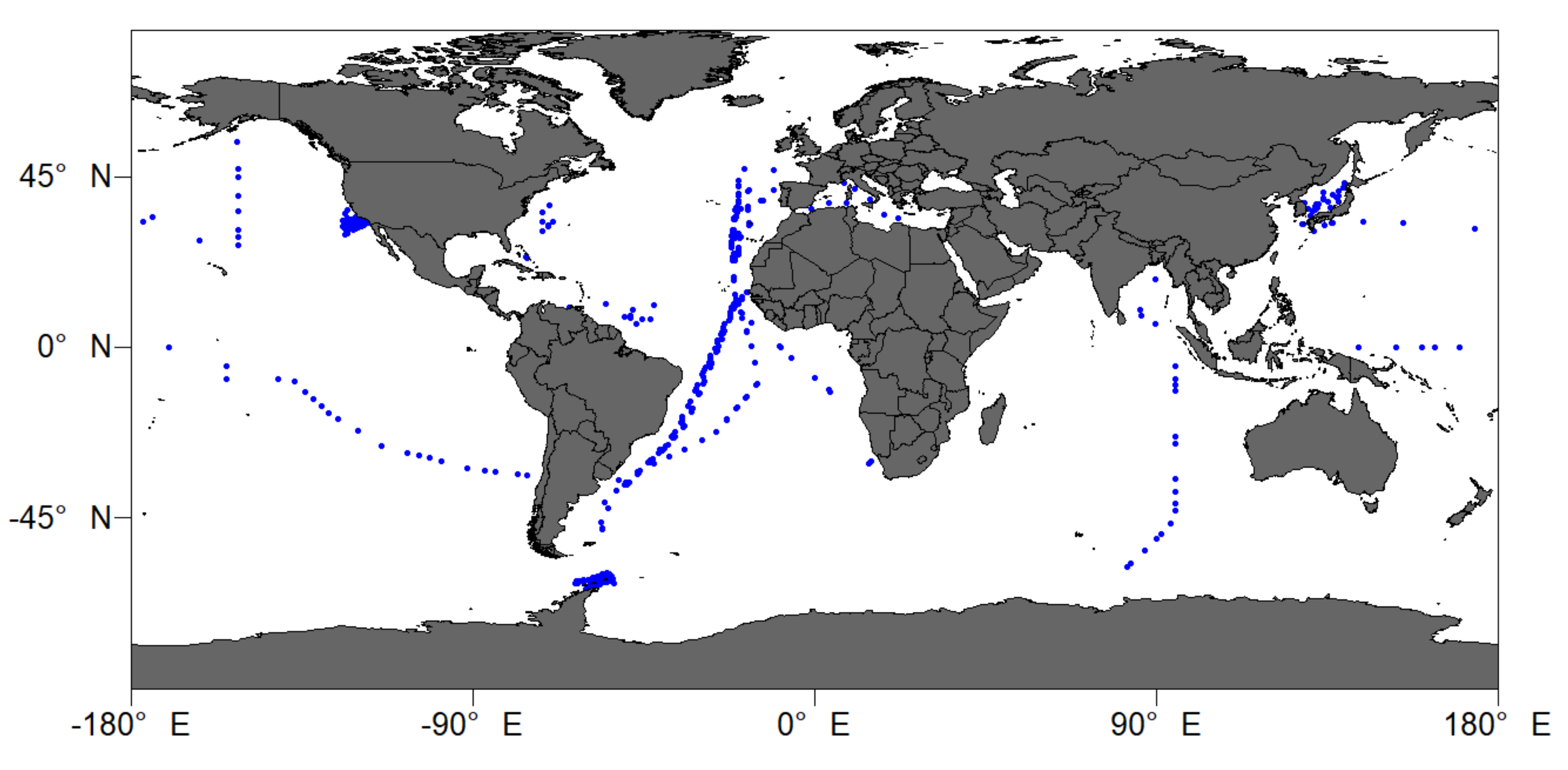
The NOMAD is quality-controlled following three steps to obtain accurate data in Case water. First, the Chla concentration was measured by high-performance liquid chromatography. Second, was measured using the in-water method. Finally, was classified according to Wei et al. [19], and types 1–4 remained. After quality control, 521 stations remained, as shown in Figure 1.
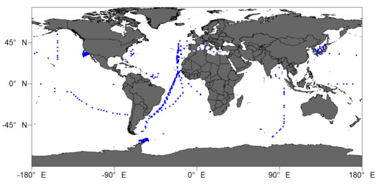
Figure 1.
Stations of the NOMAD data set.
The optical properties of case-1 water were dominated by phytoplankton, although there were also CDOM and suspended sediment. All of these were all accompanied by the death of phytoplankton. Therefore, the approximate shape of the spectrum was the same, and the spectrum decreased as the band increased. Classes 1–4 belong to this category. In natural water, there is no Case-1 water with a high chlorophyll concentration, as the nutrients required for the algae growth are imported from land sources, accompanied by CDOM and suspended sediments.
3.2. SCS Data Set
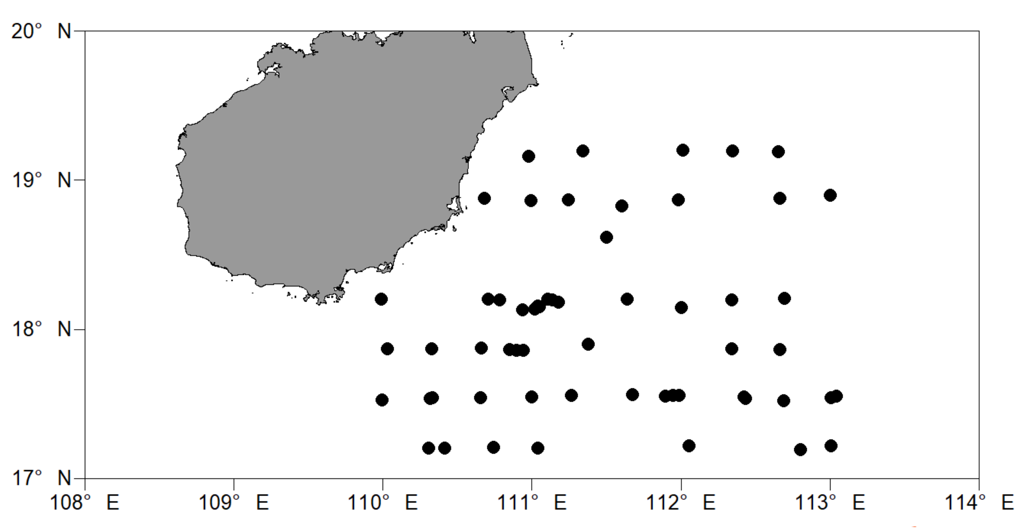
In situ data were collected from the coastal and offshore waters of the SCS (Figure 2). Most stations are situated around the Pearl River and Hainan Island. The is an in-water optical measurement obtained using HyperPro II (Satlantic), following the NASA ocean-optical protocols [20,21]. The Chla concentration was measured by high-performance liquid chromatography and it ranged from 0.0458 to 0.1869 mg m−3. The number of stations in the SCS is 58.
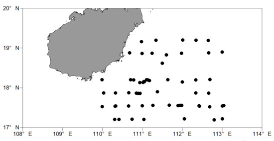
Figure 2.
Station of the South China Sea.
3.3. Statistical Method
Several statistical parameters were used to evaluate the model match-up results. The definitions of the parameters are as follows.
Bias:
Absolute percentage difference (APD):
Relative percentage difference (RPD):
where is the ith model-retrieved value, is the ith in situ value, and is the number of match-up data points.
4. Results and Discussion
4.1. Difference between the Four ORM Models
4.1.1. Difference between and of the Four ORM Models
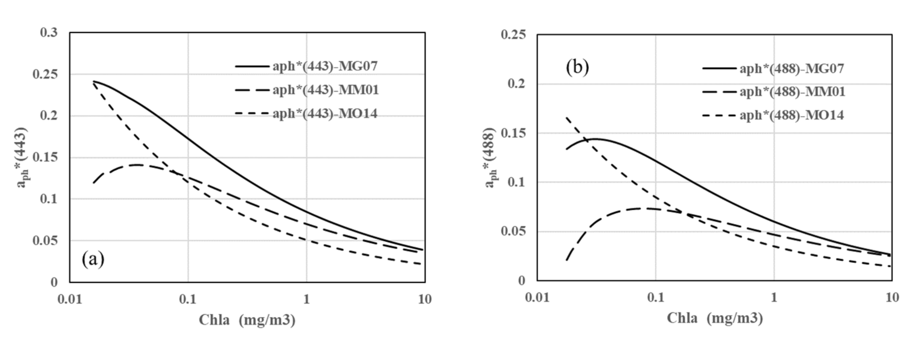
The and from the MM01, MG07 and MO14 models are shown in Figure 3. The value of of MG07 was larger than that of the other ORM models for all chlorophyll concentrations. The value of of MG07 was larger than that of the other ORM models, except when the chlorophyll concentration was less than 0.3 mg m−3. The value of of MO14 was larger than that of the other ORM models, when the chlorophyll concentration was less than 0.3 mg m−3.

Figure 3.
The and of MM01, MG07 and MO14 models with the concentration of chlorophyll. ((a) is , (b) is ).
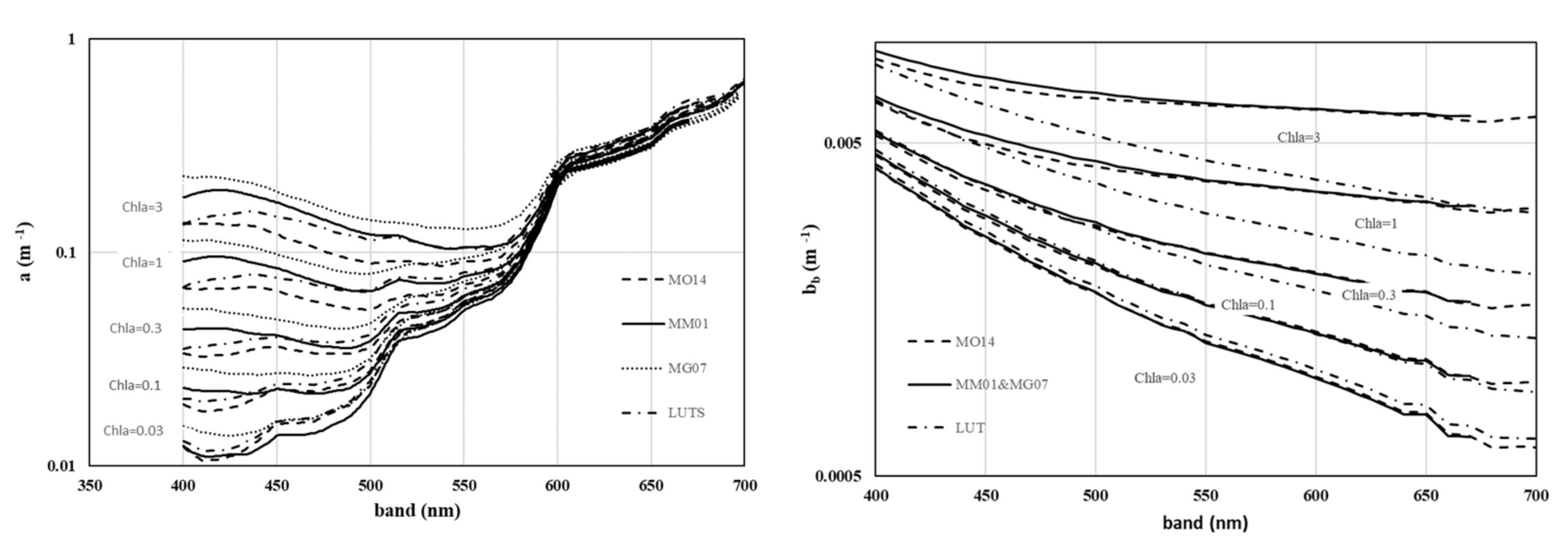
The differences in and of the G88, QAA, MG07, and L04 models are shown in Figure 4. We found that the value of of MG07 was larger than that of the other ORM models, particularly at 400–600 nm when the concentration of chlorophyll was high. The behavior of was the same for MM01 and MG07. The value of in the LUTs was less than that of the other ORM models when the concentration of chlorophyll was high.
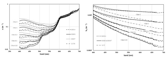
Figure 4.
Difference in and of MM01, MG07, MO14, and LUT models, when the concentration of chlorophyll is 0.03, 0.1, 0.3, 1 and 3 mg m−3 (left is , right is ).
4.1.2. Difference between the Values of the Four ORM Models
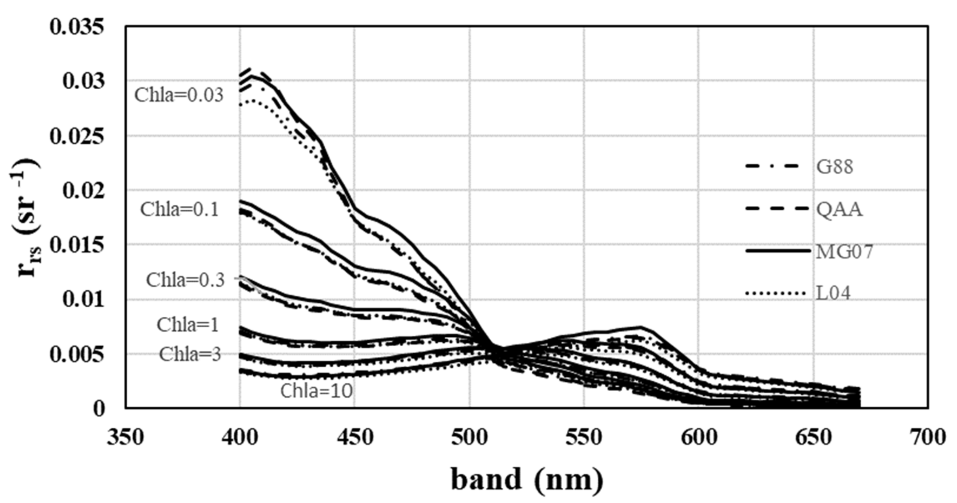
The differences in of the G88, QAA, MG07, and L04 models are shown in Figure 5. We found that the difference in was small when the concentration of chlorophyll was large. As the Chla concentration decreased, the difference became increasingly large. The difference in between QAA and GM07 reached 15% at 488 nm and 20% at 510–580 nm when the concentration of chlorophyll was 0.03 mg m−3.
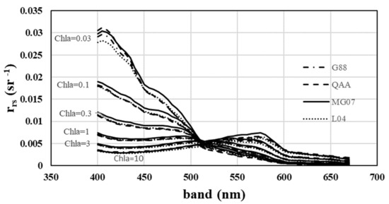
Figure 5.
Differences in of the G88, QAA, MG07, and L04 models, when the concentration of chlorophyll was 0.03, 0.1, 0.3, 1, 3 and 10 mg m−3.
4.1.3. Relationship between and
The differences in between formula (8) and ≈ 0.5291 are shown in Figure 6. The differences in between the four models are shown in Figure 7. The values of the four models were similar, particularly at 670 nm. The of MM01 was larger than that of the other models at 412 and 443 nm when the concentration of chlorophyll was less than 0.1 mg m−3. The of MO14 was larger than that of the other models when the concentration of chlorophyll was greater than 0.1 mg m−3.
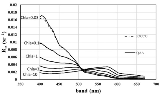
Figure 6.
Difference in between formula (8) and (IOCCG, 2006), when the concentration of chlorophyll was 0.03, 0.1, 0.3, 1, 3 and 10 mg m−3.
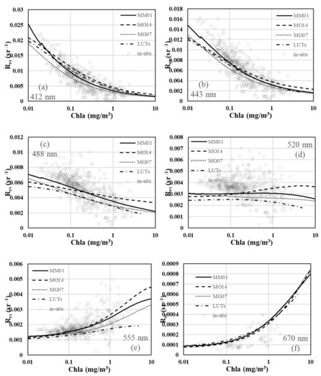
Figure 7.
Differences in between of the MM01, MG07, MO14, and LUTs models and in situ data, when the concentration of chlorophyll was 0.01–10mg m−3 ((a) 412 nm, (b) 443 nm, (c) 488 nm, (d) 510 nm, (e) 555 nm, (f) 670 nm).
4.1.4. Difference between of the Four ORM Models
4.2. Global and SCS Performances of the Four Models
The chlorophyll concentration according to NOMAD or SCS data after quality control was used as the input to the four models, and the in situ spectrum data and model output spectrum data were compared to analyze which model performed the best. The first test involved NOMAD and the second involved the SCS dataset. The scope of the in situ spectrum data was larger than that of the model output, as the data measured by the field instrument are influenced by many factors, such as the self-shadow of the instrument, error of the underwater extrapolation method, introduction error of water layering, bidirectional reflectivity, and packing effect of phytoplankton. The outputs of the models are equivalent to the outputs of theoretical analyses, and the model is not comprehensive compared to reality, particularly when simulating backscattering and CDOM absorption, and thus, variation ranges of the models are not as large as those of the data measured by field instruments.
4.2.1. Global Performance of the Four ORM Models
The differences in between the four models are shown in Figure 8. The values of the four models were similar, especially at 670 nm. The of MM01 was larger than that of the other models at 412 and 443 nm when the concentration of chlorophyll was less than 0.1 mg m−3. The of MO14 was larger than that of the other models when the concentration of chlorophyll was more than 0.1 mg m−3.
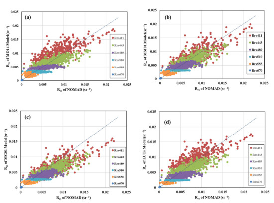
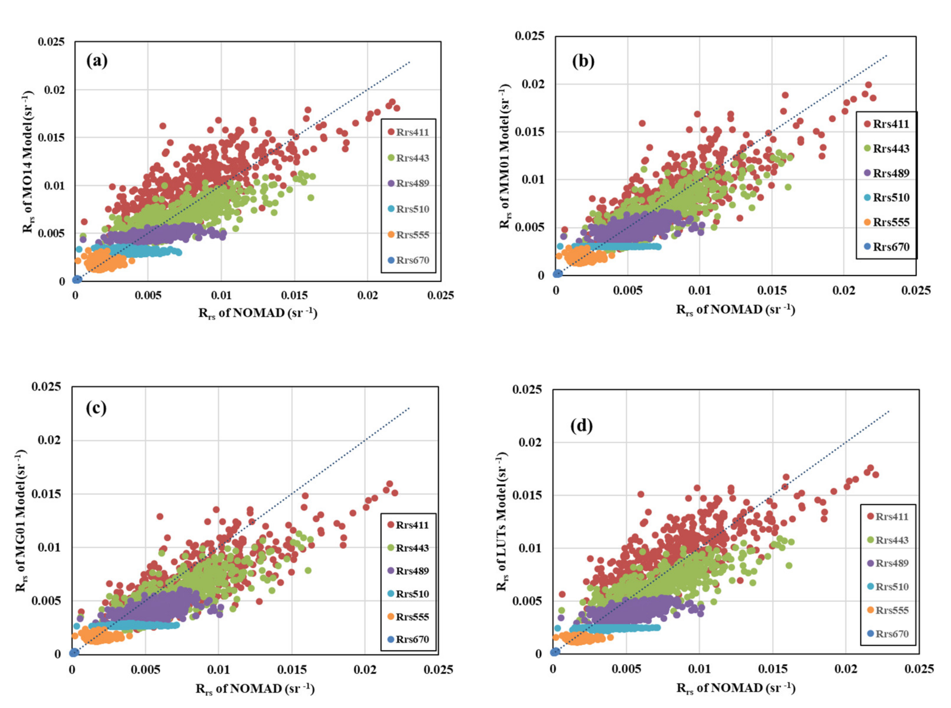
Figure 8.
Performance of MM01, MG07, MO14 and LUTs models using the NOMAD dataset ((a) MO14, (b) MM01, (c) MG07, (d) LUTs).
Comparisons between the of the four models with NOMAD data are shown in Figure 8, and the statistical parameters are listed in Table 1. The global performance of the four ORMs was good. The APD in of the four models was less than 30%, especially in the 670-nm band and a few other bands. The values of all the models were less than those of the in situ data at 443, 489, 510, and 555 nm. According to the APD, the best bands of MM01, MO14, MG07, and LUTs were 489, 489, 555 and 443 nm, respectively, which were better than 25% and 20%(MM01). For 411 nm, MG07 and MM01 were better than LUTs, and MO14 was the worst. For 443 nm, MO14 and MM01 were better than LUTs, and MG07 was the worst. For 489 and 510 nm, MO14 and MM01 were better than MG07, and LUTs was the worst. For 555 nm, MG07 and MM01 were better than MO14, and LUTs was the worst. For 670 nm, MO14 was the best, and LUTs was the worst. In the global range, MM01 was the best ORM model.

Table 1.
Statistical parameter of MM01, MG07, MO14 and LUTs models using the NOMAD dataset.
4.2.2. SCS Performance of the Four ORM Models
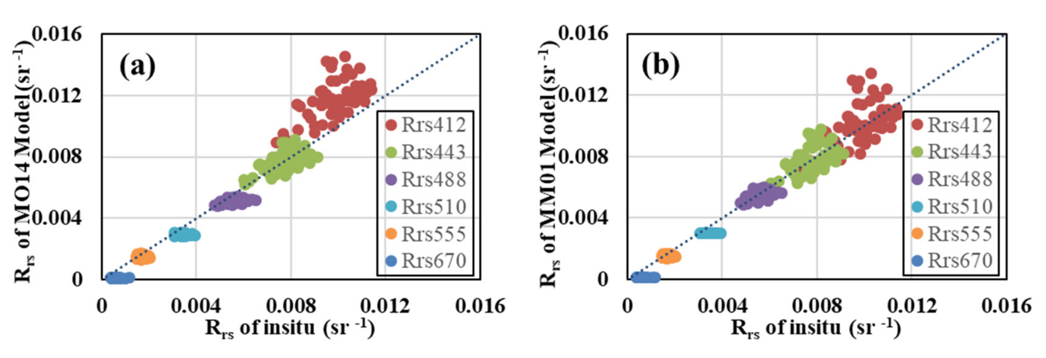
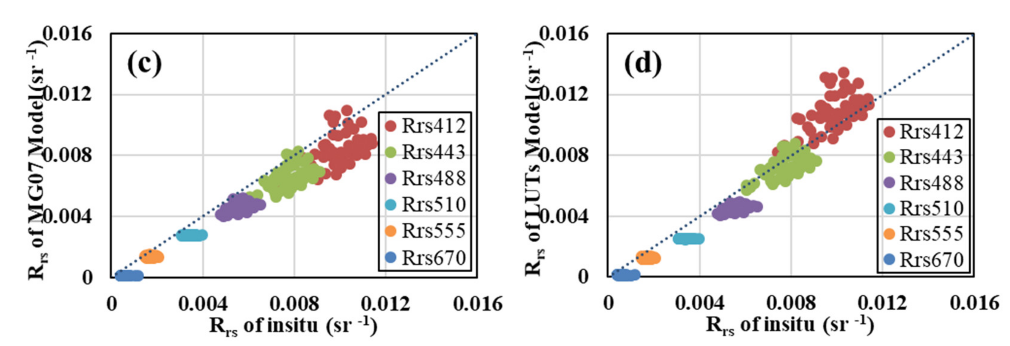
The scatter plot of the comparison between the of the four models with SCS data is shown in Figure 9, and the statistical parameters are shown in Table 2. The performances of the four ORMs were good in the SCS. The APD of of the four models was less than 30%, particularly at 670 nm. The values of all the models were less than those of the in situ data at 443, 489, 510, and 555 nm. According to APD, the best bands for MM01, MO14, MG07, and LUTs were at 443, 488, 443, and 443 nm, respectively, which were better than 17% and 6% (MM01). According to the APD, MM01 was better than 10% for 412, 443 and 488 nm. For 555 and 510 nm, MM01 was the best. For 670 nm, MM01, MG07, and LUTs were similar, and MO14 was the worst. Therefore, MM01 was the best ORM model in the SCS.
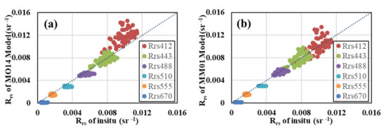
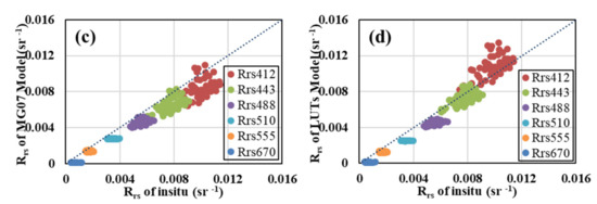
Figure 9.
Performance of MM01, MG07, MO14 and LUTs models using the dataset from the South China Sea ((a) MO14, (b) MM01, (c) MG07, (d) LUTs).
Table 2.
Statistical parameters between MM01, MG07, MO14 and LUTs models using the South China Sea dataset.
4.2.3. Performance of the Four Models at Different Chlorophyll Concentrations
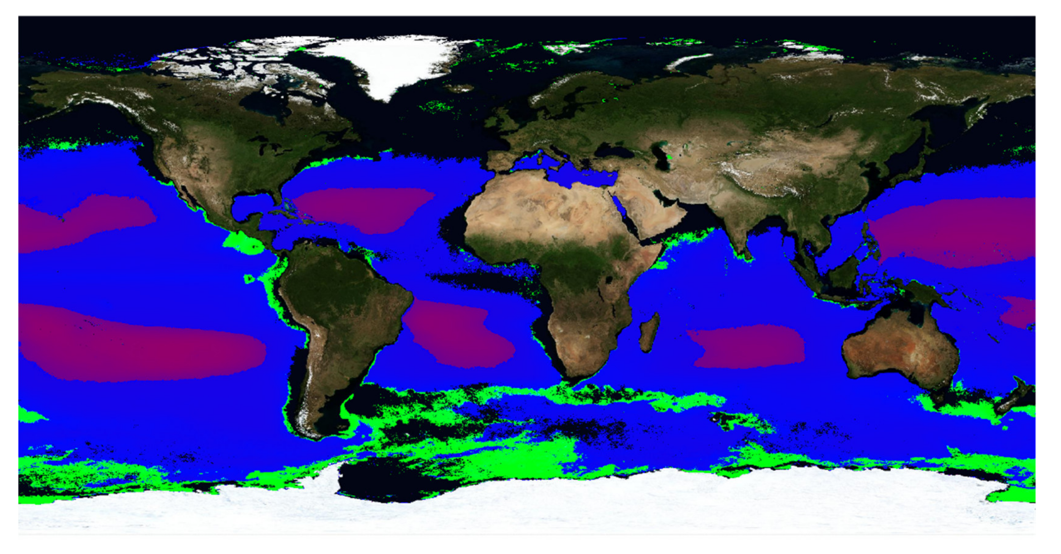
Chlorophyll concentration is the input to the ORM, and it typically related to the types of sea areas, such as oligotrophic oceans, open oceans, and coastal areas. The monthly average MODIS data (from 2002 to 2015) were used to calculate the average value of chlorophyll in the oligotrophic ocean, as shown in Figure 4.1 of Volume 14 of the IOCCG report. The mean chlorophyll was generally less than 0.07 mg m−3 in the oligotrophic ocean. The chlorophyll concentration was typically less than 0.3 mg m−3, and greater than 0.07 mg m−3 in the open ocean, such as in the SCS. The chlorophyll concentration was typically greater than 0.3 mg m−3 in coastal areas. The regions of global ocean based on the chlorophyll concentration are shown in Figure 10. Below, we discuss the performances of the four models for different chlorophyll concentrations (the figures and tables are shown in the Appendix A, Figure A1, Figure A2 and Figure A3, Table A1, Table A2 and Table A3).
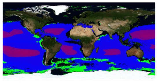
Figure 10.
Different regions of global ocean based on chlorophyll concentration (purple is oligotrophic oceans, blue is open oceans, green is coastal areas, black is Case II water).
The four models performed best in oligotrophic oceans, followed by open oceans, and coastal areas performed the worst. In oligotrophic oceans, the APDs of the four models reached 25%, excluding individual bands. In the open ocean, the APDs of the four models reached 30%, excluding individual bands. In coastal areas, the APDs of the four models were close to 50% or higher. In oligotrophic saline bodies and open oceans, the performance results of the four models were acceptable. The statistical results showed that the MM01 model was the best in open and oligotrophic oceans.
4.3. Comparison of the Chlorophyll Algorithm and ORM Models
The chlorophyll concentrations from the NOMAD or SCS data after quality control were used as the input for the four models, and the model output spectrum data and in situ spectrum data were used as the input for the chlorophyll algorithm. OC4 corresponds to running the SeaWiFS algorithm, and OC3 is based on the algorithm developed by NOMAD for SeaWiFS. First, we compared the differences between the calculation results of the different chlorophyll algorithms of the four models and measured chlorophyll on site; then compared the difference between the best model output and NOMAD field spectrum output results.
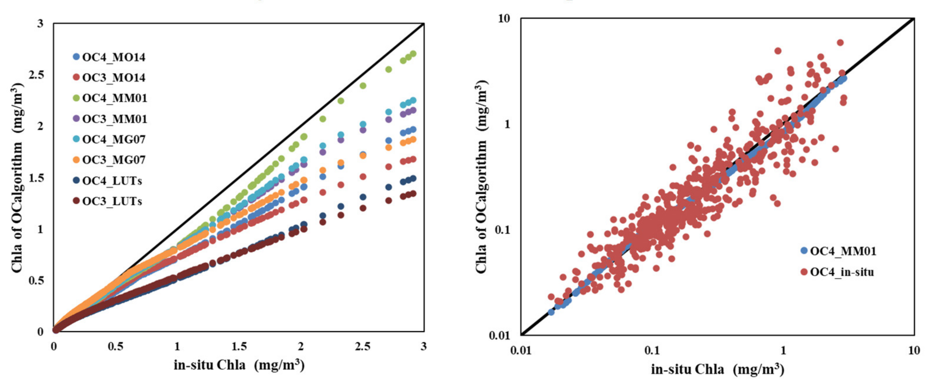
The performances of the MM01, MG07, MO14, and LUT models with the chlorophyll algorithm are shown in Figure 11 (left), and the statistical parameters of the MM01, MG07, MO14, and LUT models are shown in Table 3. By comparing the output chlorophyll results of the four models with the onsite measured chlorophyll algorithm, we found that MM01 gave the best results, regardless of whether the OC3 or OC4 chlorophyll algorithm was used. All data measured on site indicated higher chlorophyll concentrations than those indicated by results of the model. This difference was particularly notable in areas with high chlorophyll concentrations. The difference between the chlorophyll concentration output by MM01 and that measured on site was the smallest. The RPD reached below 3%, and the APD was below 10%, which was much better than that of other models for which the RPDs were approximately 7% or more and the APDs were more than 10%. Gordon et al. also verified the semi-analytic radiance model and used the model to develop a chlorophyll algorithm [22]. Lee et al. verified the forward reflectance models based on the stratification of water bodies and demonstrated the validity of the model [23]. As shown by Lee et al. [23], algorithm development and verification using surface Chla is useful, as these data are very easy to collect and generally available for all field measurements. Therefore, we only used surface Chla as the input for the ORM model.
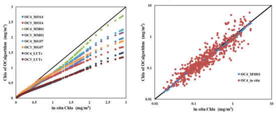
Figure 11.
Performance of the MM01, MG07, MO14, and LUT models with the chlorophyll algorithm (OC3 and OC4, left) and comparison of OC4 algorithm between MM01 and in situ spectroscopy (right).
Table 3.
Statistical parameter of chlorophyll algorithm (OC3 and OC4) between MM01, MG07, MO14, and LUT models and in situ spectrum.
The chlorophyll output results of the measured spectrum of NOMAD showed more obvious fluctuations, as shown in the scatter plot of comparisons with MM01 (Figure 10, right). The chlorophyll inverted by MM01 was mostly a straight line, and the inversion result of the NOMAD was very scattered. The statistical results of NOMAD were similar. The difference between the RPD and similar results of the model were minimal, although there was a significant difference in the APD.
5. Conclusions
Based on the NOMAD and SCS datasets, we tested and verified the four ORM models. Our conclusions were as follows:
- For the relationship between and , the four ORM models were similar at high Chla concentrations. The differences between the four ORMs increased when the Chla concentration decreased.
- In the model of the absorption coefficient, the differences between the four ORM models were large, and MG07 was overestimated compared to the others. In the backscattering coefficients model, the differences between the four ORM models were small, and LUTs underestimated the others, where the Chla concentration was high.
- Analysis of four ORM models and in situ match-ups of remote-sensing reflectance data showed that the model-derived values were less than those of the in situ data. The highest uncertainty was observed at 670 nm, and the APDs of the four ORM models were less than 30% globally and 20% in the SCS. The APD of MM01 was similar or better than 20% globally and in the SCS. The global and SCS performances of MM01 were better than those of the other models.
- The inversion effects of the models at different chlorophyll concentrations showed that the four models performed best when the chlorophyll concentration was less than 0.07 mg m−3, and chlorophyll concentration was between 0.07 and 0.3 mg m−3, and performance was poor when the chlorophyll concentration was greater than 0.3 mg m−3.
- The applicability of the four ORM models to the chlorophyll algorithm was compared, and the chlorophyll algorithm was analyzed using on-site spectrum measurements. The MM01 model performed best among all models; the RPD was below 3%, and the APD was below 10%. The performance of the on-site data for the algorithm was worse than that of all models, and the data dispersion was higher.
Author Contributions
J.L. conceived the idea and wrote the manuscript. J.L. and T.L. discussed and revised the manuscript. J.L., T.L., Q.S. and C.M. processed the in situ data. All authors have read and agreed to the published version of the manuscript.
Funding
This research was funded by the National Natural Science Foundation of China, China, Grant No. 41906172.
Acknowledgments
Acknowledgments are due to NOMAD for the distribution of in situ data. Thanks to Cédric Jamet for his help to the manuscript. Thanks also go to the reviewers for thorough comments that really helped improve the manuscript.
Conflicts of Interest
The authors declare no conflict of interest.
Appendix A

Figure A1.
Performance of MM01, MG07, MO14, and LUTs models in oligotrophic ocean ((a) MO14, (b) MM01, (c) MG07, (d) LUTs).
Figure A1.
Performance of MM01, MG07, MO14, and LUTs models in oligotrophic ocean ((a) MO14, (b) MM01, (c) MG07, (d) LUTs).
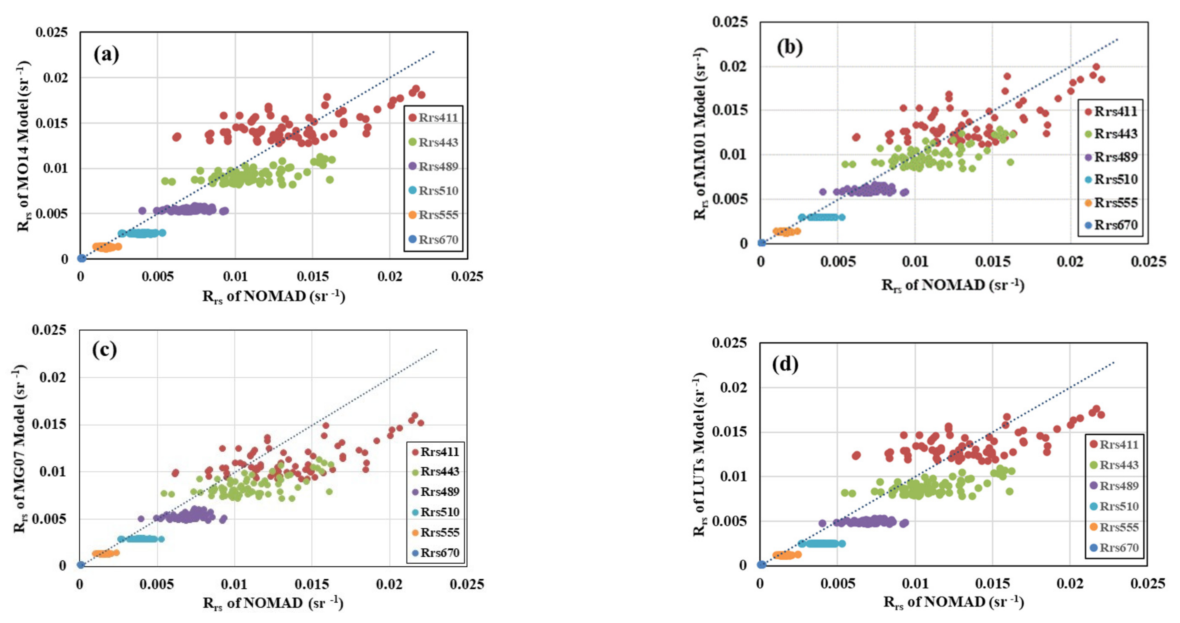
Table A1.
Statistical parameters of MM01, MG07, MO14, and LUTs models in oligotrophic ocean.
Table A1.
Statistical parameters of MM01, MG07, MO14, and LUTs models in oligotrophic ocean.
| Model | |||||||
|---|---|---|---|---|---|---|---|
| MO14 | BIAS (sr−1) | 0.00101 | −0.00189 | −0.00152 | −0.00105 | −0.00025 | −0.00001 |
| RPD (%) | 13.82 | −14.10 | −20.54 | −25.84 | −14.57 | −1.93 | |
| APD (%) | 22.70 | 18.83 | 21.68 | 26.27 | 16.78 | 17.30 | |
| MM01 | BIAS (sr−1) | 0.00006 | −0.00119 | −0.00090 | −0.00088 | −0.00020 | 0.00001 |
| RPD (%) | 5.65 | −7.81 | −11.63 | −21.53 | −10.96 | 7.62 | |
| APD (%) | 20.23 | 15.69 | 14.39 | 22.40 | 14.28 | 20.17 | |
| MG07 | BIAS (sr−1) | −0.00248 | −0.00265 | −0.00172 | −0.00105 | −0.00027 | 0.00001 |
| RPD (%) | −13.87 | −21.55 | −23.59 | −25.89 | −15.67 | 8.45 | |
| APD (%) | 22.19 | 24.06 | 24.31 | 26.22 | 17.27 | 19.30 | |
| LUTs | BIAS (sr−1) | −0.00007 | −0.00224 | −0.00202 | −0.00140 | −0.00038 | 0.00001 |
| RPD (%) | 5.39 | −17.43 | −27.93 | −34.95 | −22.86 | 18.35 | |
| APD (%) | 20.37 | 21.02 | 28.46 | 34.95 | 23.46 | 24.44 | |
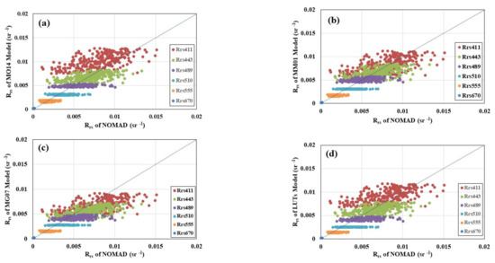
Figure A2.
Performance of MM01, MG07, MO14, and LUTs models in open ocean ((a) MO14, (b) MM01, (c) MG07, (d) LUTs).
Figure A2.
Performance of MM01, MG07, MO14, and LUTs models in open ocean ((a) MO14, (b) MM01, (c) MG07, (d) LUTs).
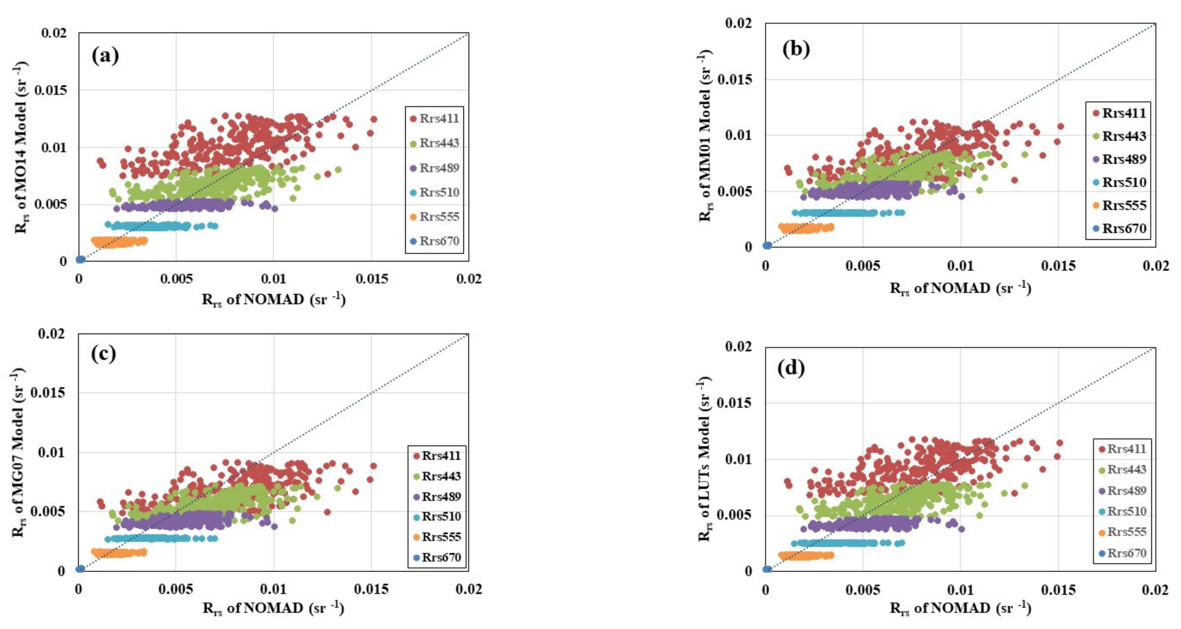
Table A2.
Statistical parameters of MM01, MG07, MO14, and LUTs models in open ocean.
Table A2.
Statistical parameters of MM01, MG07, MO14, and LUTs models in open ocean.
| Model | |||||||
|---|---|---|---|---|---|---|---|
| MO14 | BIAS (sr−1) | 0.00205 | −0.00020 | −0.00064 | −0.00064 | −0.00006 | 0.00003 |
| RPD (%) | 45.90 | 7.16 | −5.78 | −13.19 | 0.46 | 45.15 | |
| APD (%) | 49.24 | 24.54 | 20.55 | 21.00 | 15.45 | 49.38 | |
| MM01 | BIAS (sr−1) | 0.00032 | −0.00038 | −0.00046 | −0.00063 | −0.00005 | 0.00004 |
| RPD (%) | 19.54 | 3.62 | −2.68 | −13.09 | 1.04 | 57.03 | |
| APD (%) | 33.28 | 23.43 | 18.74 | 20.35 | 15.18 | 59.29 | |
| MG07 | BIAS (sr−1) | −0.00115 | −0.00140 | −0.00132 | −0.00092 | −0.00021 | 0.00004 |
| RPD (%) | −1.70 | −12.56 | −19.10 | −21.55 | −8.88 | 58.48 | |
| APD (%) | 30.97 | 27.10 | 25.84 | 25.39 | 16.24 | 60.62 | |
| LUTs | BIAS (sr−1) | 0.00121 | −0.00067 | −0.00130 | −0.00117 | −0.00034 | 0.00006 |
| RPD (%) | 33.40 | −0.65 | −18.68 | −28.52 | −16.44 | 75.29 | |
| APD (%) | 40.37 | 24.23 | 25.83 | 30.81 | 20.41 | 76.24 | |
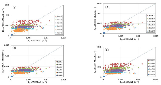
Figure A3.
Performance of MM01, MG07, MO14, and LUTs models in coastal area ((a) MO14, (b) MM01, (c) MG07, (d) LUTs).
Figure A3.
Performance of MM01, MG07, MO14, and LUTs models in coastal area ((a) MO14, (b) MM01, (c) MG07, (d) LUTs).
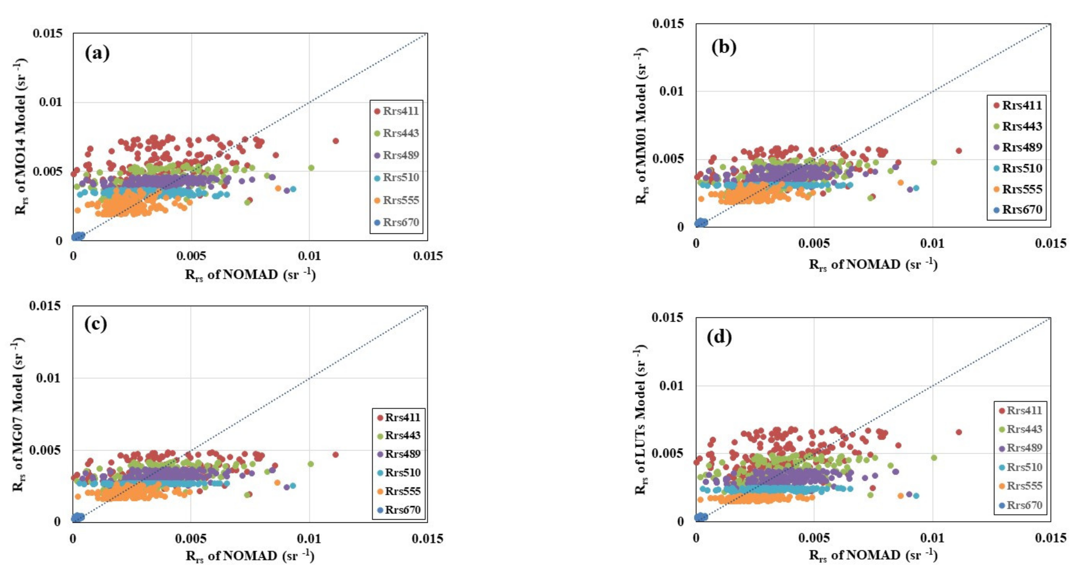
Table A3.
Statistical parameters of MM01, MG07, MO14 and LUTs models in coastal area.
Table A3.
Statistical parameters of MM01, MG07, MO14 and LUTs models in coastal area.
| Model | ||||||
|---|---|---|---|---|---|---|
| MO14 | BIAS (sr−1) | 0.00170 | 0.00073 | 0.00056 | 0.00021 | 0.00020 |
| RPD (%) | 229.39 | 80.96 | 49.75 | 33.38 | 26.50 | |
| APD (%) | 234.39 | 90.69 | 60.21 | 48.17 | 39.12 | |
| MM01 | BIAS (sr−1) | 0.00046 | 0.00016 | 0.00013 | −0.00016 | 0.00004 |
| RPD (%) | 151.66 | 54.94 | 33.40 | 18.71 | 18.73 | |
| APD (%) | 168.93 | 73.73 | 50.16 | 41.50 | 34.73 | |
| MG07 | BIAS (sr−1) | −0.00023 | −0.00037 | −0.00050 | −0.00056 | −0.00031 |
| RPD (%) | 110.50 | 32.44 | 11.14 | 2.98 | 0.49 | |
| APD (%) | 140.44 | 63.58 | 43.35 | 39.46 | 29.59 | |
| LUTs | BIAS (sr−1) | 0.00117 | 0.00010 | −0.00055 | −0.00088 | −0.00059 |
| RPD (%) | 196.22 | 52.11 | 8.65 | −9.59 | −13.47 | |
| APD (%) | 204.90 | 72.30 | 42.91 | 40.96 | 31.48 | |
References
- Platt, T.; Hoepffner, N.; Stuart, V.; Brown, C. (Eds.) IOCCG Report Number 7: Why Ocean Colour? The Societal Benefits of Ocean-Colour Technology; Reports of the International Ocean-Colour Coordinating Group: Dartmouth, NS, Canada, 2008. [Google Scholar]
- Morel, A.; Huot, Y.; Gentili, B.; Werdell, P.J.; Hooker, S.B.; Franz, B.A. Examining the consistency of products derived from various ocean color sensors in open ocean (Case 1) waters in the perspective of a multi-sensor approach—Science Direct. Remote Sens. Environ. 2007, 111, 69–88. [Google Scholar] [CrossRef]
- Franz, B.A.; Bailey, S.W.; Werdell, P.J.; Mcclain, C.R. Sensor-independent approach to the vicarious calibration of satellite ocean color radiometry. Appl. Opt. 2007, 46, 5068–5082. [Google Scholar] [CrossRef] [PubMed]
- Hooker, S.B.; Bernhard, G.; Morrow, J.H.; Booth, C.R.; Comer, T.; Lind, R.N.; Quang, V. Optical Sensors for Planetary Radiant Energy (OSPREy): Calibration and Validation of Current and Next-Generation NASA Missions; NASA Technology Memo: Greenbelt, MD, USA, 2012; pp. 1–177. [Google Scholar]
- Morel, A.; Claustre, H.; Antoine, D.; Gentili, B. Natural variability of bio-optical properties in Case 1 waters: Attenuation and reflectance within the visible and near-UV spectral domains, as observed in South Pacific and Mediterranean waters. Biogeosciences 2007, 4, 913–925. [Google Scholar] [CrossRef] [Green Version]
- Lee, Z.; Carder, K.L.; Du, K. Effects of molecular and particle scatterings on the model parameter for remote-sensing reflectance. Appl. Opt. 2004, 43, 4957–4964. [Google Scholar] [CrossRef] [PubMed] [Green Version]
- Lee, Z.P. (Ed.) IOCCG Report Number 5: Remote Sensing of Inherent Optical Properties: Fundamentals, Tests of Algorithms, and Applications; Reports of the International Ocean-Colour Coordinating Group: Dartmouth, NS, Canada, 2006; pp. 1–122. [Google Scholar]
- Morel, A.; Loisel, H. Apparent optical properties of oceanic water: Dependence on the molecular scattering contribution. Appl. Opt. 1998, 37, 4765–4776. [Google Scholar] [CrossRef] [PubMed] [Green Version]
- Morel, A. Optical modeling of the upper ocean in relation to its biogenous matter content (case I waters). J. Geophys. Res. Atmos. 1988, 931, 10749–10768. [Google Scholar] [CrossRef] [Green Version]
- Morel, A.; Maritorena, S. Bio-optical properties of oceanic waters: A reappraisal. J. Geophys. Res. Ocean. 2001, 106, 7163–7180. [Google Scholar] [CrossRef] [Green Version]
- Morel, A.; Gentili, B.; Claustre, H.; Babin, M.; Bricaud, A.; Tièche, R. Optical Properties of the “Clearest” Natural Waters. Limnol. Oceanogr. 2007, 52, 217–229. [Google Scholar] [CrossRef]
- A New IOP Model for Case 1 Water. Available online: https://www.oceanopticsbook.info/view/optical-constituents-of-the-ocean/level-2/new-iop-model-case-1-water (accessed on 12 July 2021).
- Mobley, C.D.; Sundman, L.K. Hydrolight 5 Ecolight 5; Sequoia Scientific Inc.: Bellevue, WA, USA, 2008; pp. 1–95. [Google Scholar]
- Gordon, H.R.; Clark, D.K. Clear water radiances for atmospheric correction of coastal zone color scanner imagery. Appl. Opt. 1981, 20, 4175–4180. [Google Scholar] [CrossRef] [PubMed]
- An Update of the Quasi-Analytical Algorithm (QAA_v5); Technical Report: International Ocean Colour Coordinating Group (IOCCG). Available online: https://www.ioccg.org/groups/Software_OCA/QAA_v5.pdf (accessed on 12 July 2021).
- Smith, R.C.; Baker, K.S. The Bio-Optical State of Ocean Waters and Remote Sensing. Limnol. Oceanogr. 1978, 23, 247–259. [Google Scholar] [CrossRef] [Green Version]
- Pope, R.M.; Fry, E.S. Absorption spectrum (380–700 nm) of pure water. II. Integrating cavity measurements. Appl. Opt. 1997, 36, 8710–8723. [Google Scholar] [CrossRef] [PubMed]
- Mobley, C.D.; Sundman, L.K.; Davis, C.O.; Bowles, J.H.; Gleason, A. Interpretation of hyperspectral remote-sensing imagery by spectrum matching and look-up tables. Appl. Opt. 2005, 44, 3576–3592. [Google Scholar] [CrossRef] [PubMed]
- Wei, J.; Lee, Z.; Shang, S. A system to measure the data quality of spectral remote sensing reflectance of aquatic environments. J. Geophys. Res. Ocean. 2016, 121. [Google Scholar] [CrossRef]
- Mueller, J.L.; Fargion, G.S.; Mcclain, C.R. Ocean Optical Protocols for Satellite Ocean Color Sensor Vlidation; Revision 3; NASA Technology Memo: Greenbelt, MD, USA, 2003; pp. 1–137. [Google Scholar]
- Morel, A.; Mueller, J.L. Normalized Water-Leaving Radiance and Remote Sensing Reflectance: Bidirectional Reflectance and Other Factors in Ocean Optics Protocols for Satellite Ocean Color Sensor Validation; Revision 3; NASA Technology Memo: Greenbelt, MD, USA, 2002; pp. 1–137. [Google Scholar]
- Gordon, H.R.; Brown, O.B.; Evans, R.H.; Brown, J.W.; Smith, R.C.; Baker, K.S.; Clark, D.K. A semianalytic radiance model of ocean color. J. Geophys. Res. 1988, 93, 10909–10924. [Google Scholar] [CrossRef]
- Lee, Z.; Wang, Y.; Yu, X.; Shang, S.; Luis, K. Evaluation of forward reflectance models and empirical algorithms for chlorophyll concentration of stratified waters. Appl. Opt. 2020, 59, 9340–9352. [Google Scholar] [CrossRef] [PubMed]


Publisher’s Note: MDPI stays neutral with regard to jurisdictional claims in published maps and institutional affiliations. |
© 2021 by the authors. Licensee MDPI, Basel, Switzerland. This article is an open access article distributed under the terms and conditions of the Creative Commons Attribution (CC BY) license (https://creativecommons.org/licenses/by/4.0/).