Abstract
Accurate and reliable crop classification information is a significant data source for agricultural monitoring and food security evaluation research. It is well-known that polarimetric synthetic aperture radar (PolSAR) data provides ample information for crop classification. Moreover, multi-temporal PolSAR data can further increase classification accuracies since the crops show different external forms as they grow up. In this paper, we distinguish the crop types with multi-temporal PolSAR data. First, due to the “dimension disaster” of multi-temporal PolSAR data caused by excessive scattering parameters, a neural network of sparse auto-encoder with non-negativity constraint (NC-SAE) was employed to compress the data, yielding efficient features for accurate classification. Second, a novel crop discrimination network with multi-scale features (MSCDN) was constructed to improve the classification performance, which is proved to be superior to the popular classifiers of convolutional neural networks (CNN) and support vector machine (SVM). The performances of the proposed method were evaluated and compared with the traditional methods by using simulated Sentinel-1 data provided by European Space Agency (ESA). For the final classification results of the proposed method, its overall accuracy and kappa coefficient reaches 99.33% and 99.19%, respectively, which were almost 5% and 6% higher than the CNN method. The classification results indicate that the proposed methodology is promising for practical use in agricultural applications.
1. Introduction
Crop classification plays an important role in remote sensing monitoring of agricultural conditions, and it is a premise for further monitoring of crop growth and yields [1,2]. Once the categories, areas and space distribution information of crops have been acquired in a timely and accurate manner, it can provide scientific evidence of reasonable adjustment for agriculture structure. Therefore, crop classification has great significance for guidance of agriculture production, rational distribution of farming resources and guarantee of national food security [3,4,5].
With the continuous advancement and development of remote sensing technology and its theory, it has been extensively applied in agricultural fields such as crop census, growing monitoring, yield prediction and disaster assessment [6,7,8,9]. Over the past several years, optical remote sensing has been widely applied in crop classification due to its objectivity, accuracy, wide monitoring range and low cost [10]. For example, Tatsumi adopted random forest classifier to classify the eight class crops in southern Peru of time-series Landsat 7 ETM + data, the final overall accuracy and the kappa coefficient were 81% and 0.70, respectively [11]. However, optical remote sensing data is susceptible to cloud and shadow interference during the collection, so it is difficult to obtain effective continuous optical remote sensing data in the critical period of crop morphological changes. In addition, optical remote sensing data only reflect the spectral signature of target surface. For the wide variety of ground objects, there exists the phenomenon of “same object with different spectra and different objects with the same spectrum”. Therefore, the crop classification accuracy based on optical remote sensing data is limited to a certain extent. Unlike the optical remote sensing, PolSAR is an active microwave remote sensing technology, its working conditions cannot be restricted by weather and climate. Meanwhile, besides the signature of target surface, SAR remote sensing data provide other spectral signatures of target due to its penetrability. Therefore, increasing amounts of attention has been paid to the research with PolSAR data in crop classification [12,13]. However, the constraints of developing level for radar technology, the majority of classification research for crops used single-temporal PolSAR data. However, as for crop categories, identification, single-temporal PolSAR image offers only limited information for crops. Therefore, it is very difficult to identify different crop categories due to the same external phenomena in the certain period, especially during the sowing period [14]. Therefore, it is necessary to collect multi-temporal PolSAR data to further improve the crop classification accuracy.
In recent two decades, an increasing number of satellite-borne SAR systems have been launched successfully and operate on-orbit, which made it available to acquire multi-temporal remote sensing data for desired target [15,16,17]. At present, there are several representative systems available for civilian applications, such as L-band Uninhabited Aerial Vehicle Synthetic Aperture Radar (UAVSAR) [18], C-band Sentinel-1 [19,20], GF-3, RADARSAT-2 and Radarsat Constellation Mission (RCM) [21], and X-band Constellation of Small Satellites for Mediterranean basin observation (COSMO) and COSMO-SkyMed 2nd Generation (CSG) [22]. Through these on-orbit SAR systems, a number of multi-temporal PolSAR images for the same area can be readily acquired for crop surveillance and other related applications. Additionally, it can show different scattering characteristics for crops in different growing periods, which greatly improves the classification accuracy of crops [23,24,25].
Recently, a number of classification algorithms with PolSAR data have been presented in the literature, which can be roughly divided into three categories:
- (1)
- Algorithms based on statistical models [26]. For example, Lee et al. proposed a classical classifier based on the complex Wishart distribution [27];
- (2)
- Algorithms based on the scattering mechanisms of polarization [28]. The points with the same physical meaning are classified using the polarization scattering parameters obtained by the coherent and incoherent decomposition algorithms (such as Pauli decomposition [29], Freeman decomposition [30], etc.) [31,32,33,34,35];
- (3)
- The classification schemes based on machine learning [36], e.g., support vector machine (SVM) [37] and various neural networks [38]. For instance, Zeyada et al. use the SVM to classify four crops (rice, maize, grape and cotton) in the Nile Delta, Egypt [39].
With the collection of multi-temporal PolSAR data, the various classification algorithms based on time-series information have also been developed. For example, long short-term memory (LSTM) network has been exploited to recognize and classify the multi-temporal PolSAR images [40]. Zhong et al. classify the summer crops in Yolo County, California using the LSTM algorithm with Landsat Enhanced Vegetation Index (EVI) time series [25]. It can be seen that the research and application of multi-temporal PolSAR data are constantly progressing. For LSTM algorithm, the performance of this network mainly depends on input features, so a large amount of decomposition algorithms have been developed to extract the polarization scattering characteristics [41,42,43,44]. However, the direct use of polarization features will result in the so-called “dimension disaster” problem for the various classifiers. Therefore, the dimension reduction for the extracted multi-temporal features has become a significant work.
Some methods, such as principle component analysis (PCA) [45] and locally linear embedded (LLE) [46], etc., are popular for feature compression to solve the “dimension disaster” problem. For instance, the PCA method actually provides the optimal linear solution for data compression in the sense of minimum mean square error (MMSE) [47]. The advantage of PCA lies in the fast restoration of original data by subspace projection at a cost of minimum error. However, it cannot be guaranteed that the principle components extracted by PCA provide the most relevant information for crop type discrimination. Independent Component Analysis (ICA) is the generalization of PCA, which can gain independent gains. Bartlett M.S. et al. adopt the ICA to recognize the face images of the FERET face database [48]. Tensor decomposition is often used to extract certain elementary features from image data. Dehghanpoor G. et al. used tensor decomposition method to achieve the feature learning on satellite imagery [49]. Non-negative matrix factorization (NMF) is based on non-negative constraints, which allows learn parts from objects. Ren J.M. et al. applied the reduce dimensionality method NMF as the preprocessing of remote sensing imagery classification [50]. However, they are not suitable for dimensionality reduction about PolSAR data of crops. Additionally, the LLE method can voluntarily extract the low-dimensional feature of nonlinear from high-dimensional data, but it is very sensitive to outliers [51]. In most recent years, with the development of deep learning, the convolutional neural network (CNN) has been gradually applied in remote sensing data analysis [52]. At present, some successful network structures (e.g., auto-encoder [53,54] and sparse auto-encoder (SAE) [17,55].) have been presented, yielding excellent performances in feature compression and image classification. However, the sparsity for the SAE network has not been fully exploited to further extract efficient features for classification, and the existing CNN based classifier do not utilize the multi-scale features of the compressed data. Due to these disadvantages, the crop classification performance still cannot achieve a level for practical use.
Therefore, the main purpose of this study is to propose a new method to improve the performances of crop classification for better application in agricultural monitoring. Firstly, we adopted various coherent and incoherent scattering decomposition algorithms to extract particular parameters from multi-temporal PolSAR data. Secondly, a sparse auto-encoder network with non-negativity constraint (NC-SAE) was bulit to perform feature dimension reduction, which extracts the polarimetric features more efficiently. Finally, a classifier based on crop discrimination network with multi-scale features (MSCDN) was proposed to implement the crop classification, which greatly enhanced the classification accuracy. The main contributions of this paper were to propose a NC-SAE for data compression and a MSCDN for crop discrimination.
The remainder of this paper is organized as follows. Section 2 devotes to our methodology, including the structure of PolSAR data, the polarimetric features decomposition and dimension reduction with proposed NC-SAE network, as well as the architecture of the proposed MSCDN classifier. In Section 3, the experimental results of crop classification for the proposed method are evaluated and compared with traditional method using simulated Sentinel-1 data. Finally, Section 4 concludes the study.
2. Methodology
In order to use the multi-temporal PolSAR data to classify crops, a neural network NC-SAE was employed to compress the data, and then a novel crop discrimination network with multi-scale features (MSCDN) was constructed to achieve the crop classification. The flowchart of the whole study method is shown in Figure 1, which mainly includes three steps: polarization feature decomposition, feature compression and crop classification.
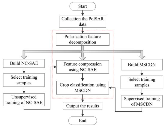
Figure 1.
Flowchart of the whole study method.
2.1. PolSAR Data Structure
The quad-pol SAR receives target backscattering signals and measures the amplitudes and phases in terms of four combinations: HH, HV, VH and VV, where H represents horizontal mode and V represents vertical mode. A 2 × 2 complex matrix that collects the scattering information can be obtained for each pixel, these complex numbers relate the incident and the scattered electric fields. The scattering matrix usually reads:
where denotes the scattering factor of vertical transmitting and horizontal receiving polarization, and the others have similar definitions.
The target feature vector can be readily obtained by vectorizing the scattering matrix. Reciprocal backscattering assumption is commonly exploited, then is approximately equal to and the polarimetric scattering matrix can be rewritten as the Lexicographic scattering vector:
where the superscript denotes the transpose of vector. The scale factor on is to ensure consistency in the span computation. Then, a polarimetric covariance matrix can be constructed as the following format:
where the superscript denotes the conjugate of a complex number. Alternatively the Pauli-based scattering vector is defined as
By using vector , a coherency matrix can be constructed as follows:
where indicates the number of looks. The coherency matrix is usually spatially averaged to reduce the inherent speckle noise in the SAR data. This preserves the phase information between the polarization channels.
The covariance matrix has been proved to follow a complex Wishart distribution, while the coherency matrix contains the equivalent information of the same PolSAR data. They can be easily converted to each other by a bilinear transformation as follows
where is a constant matrix:
2.2. Polarization Decomposition and Feature Extraction
Processing and analyzing the PolSAR data can effectively extract the polarization scattering features, and further achieve classification, detection and identification of quad-Pol SAR data. Therefore, polarization decomposition for PolSAR data is usually adopted to obtain multi-dimensional features. Here, we propose to consider the 36-dimensional polarimetric scattering features, which were derived from a single temporal PolSAR image using various methods. Some of these features can be directly obtained from the measured data, and others were computed with incoherent decomposition (i.e., Freeman decomposition [32], Yamaguchi decomposition [33], Cloude decomposition [34] and Huynen decomposition [35]) and Null angle parameters [52]. The 36-dimensional scattering features obtained from a single temporal PolSAR image are summarized in Table 1. Then, higher dimensional scattering features can be obtained from multiple temporal PolSAR images. The resulting features involve all the potential information of the primitive PolSAR data.

Table 1.
The 36-dimensional decomposition features of single-temporal PolSAR data.
2.3. Feature Compression
Directly classifying the crops with higher dimensional features above is cumbersome, which involves complicated computations and large amount of memory to store the features, and these enormous features would suffer from the great difficulty of the dimensionality disaster. Therefore, to make full use of the wealth of multiple temporal PolSAR data, the dimension reduction in resulting features is indispensable and crucial. In the past few years, the methods of auto-encoder and sparse auto-encoder have attracted more and more attention, which were commonly used to perform the compression of high-dimension data [17,55,56,57]. Therefore, the sparse auto-encoder with non-negativity constraint was proposed to further improve the sparsity of auto-encoder.
2.3.1. Auto-Encoder
An auto-encoder (AE) is a neural network which is an unsupervised learning for data representation and its aim is to set the output values approximately equal to the inputs. The basic structure of a single-layer AE neural network consists of three parts: encoder, activation and decoder, which are shown in Figure 2, where the input layer (), hidden layer () and output layer () have, respectively, neurons, neurons, and neurons. The hidden layer is commonly used to implement the encoding for the input data, while the output layer is for the decoding operation.
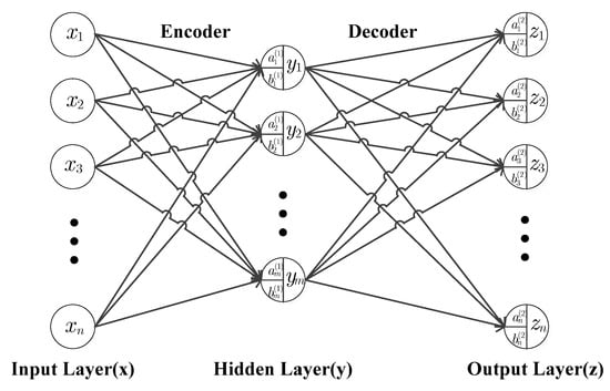
Figure 2.
Single-layer AE neural networks structure.
The weighted input of each neuron in encoder is defined as
where represents the encoder weight coefficient, is the bias of neuron Then, the encoder output can be written as the nonlinear activation of weighted input as follows
where is a sigmoid function, which is usually chosen as the logsig function:
If , the output can be viewed as the compressed representation of input , then the encoder usually plays the role of data compression. Whereas the decoder is a reverse process of reconstructing the compressed data , which achieves the restoration of the original data, i.e., output represents the estimate of input . The weighted input of the decoder is defined as
where is the decoding weight coefficient, and is the bias of neuron . The decoder output reads
Here, is the sigmoid function for decoder neurons, which is commonly chosen the same as .
The training process of AE is based on the optimization of the cost function and obtained the optimal parameters of weight coefficients and bias. The cost function measures the error between the input and its reconstruction at the output , which can be written as
where is the number of samples. Furthermore, a restriction term of weight decay is usually incorporated into the cost function to regulate the degree of the weight attenuation, which helps to effectively avoid overfitting and remarkably improve the generalization capacity for the network. Hence, the overall cost function of AE commonly reads
where is a regularization term on the weights, the most commonly used restriction is the regularization term and is defined as follows, is the coefficient for regularization term.
where is the number of layers. The weight coefficients and biases are optimized and trained by using the steepest descent algorithm via the classical error back propagation scheme.
2.3.2. Sparse Auto-Encoder with Non-Negativity Constraint
A sparse auto-encoder (SAE) results from an auto-encoder (AE). Based on AE, SAE neural network is achieved by enforcing a sparsity constraint of the output from the hidden layer, which realizes the inhibitory effects and yields fast convergence speed for training process using the back propagation algorithm [17,55]. Hence, the cost function of SAE is given by
where is the coefficient of the sparsity regularization term, is the sparsity regularization term which is usually represented by Kullback–Leibler (KL) divergence [17,55].
The part-based representation of input data usually exhibits excellent performance for pattern classification. The sparse representation scheme usually breaks the input data into parts, while the original input data can be readily reconstructed by combining the parts additively when necessary. Therefore, the input in each layer of an auto-encoder can be divided into parts by enforcing the weight coefficients of both encoder and decoder to be positive [56]. To achieve a better performance in reconstruction, we propose to consider the sparse auto-encoder with non-negativity constraint (NC-SAE), the auto encoder network decompose the input into parts by encoder via (8 and 9), and combine them in an additive manner by decoder via (11 and 12). This is achieved by replacing the regularization term (15) in cost function (16) with a new non-negativity constraint
where
Therefore, the proposed cost function for NC-SAE is defined as
where is the parameter of the non-negativity constraint. By minimizing the cost function (19), the number of nonnegative weights of each layer and the sparsity of the hidden layer activation are all increased, and the overall average reconstruction error is reduced.
Further, steepest descent method is used to update the weight and bias of (19) as follows
where is the number of iteration, and denotes the learning rate. Then, we adopt the error back-propagation algorithm to compute the partial derivatives in (20). The partial derivatives of the cost function with respect to decoder reads
The partial derivatives in (21) are straightforward, and shown below
where is shown as follows
In order to clarify the computation of derivatives, we define the neuronal error as the derivative of cost function with respect to weight input of each neuron, i.e., . Then, can be calculated using the chain rule as follows:
Similarly, the neuronal error of encoder is computed as
Now substituting Equations (22) and (24) into (21) leads to
Then, the partial derivative of the cost function with respect to the encoding weight reads
The partial derivatives with respect to the biases of encoder and decoder are computed in a compact form as
2.4. The Crop Discrimination Network with Multi-Scale Features (MSCDN)
In the deep learning field, convolutional neural network (CNN) has become increasingly powerful to deal with the complicated classification and recognition problems. Recently, CNN has been widely adopted in remote sensing, for example, in image classification, target detection, and semantic segmentation. However, most classical CNNs only use one single convolution kernel to extract the feature images, the resulting single feature map in each convolutional layer make it difficult to distinguish the similar crops, consequently the overall crop classification performance degraded. Just as our previous work [17], the poor overall performance is devoted to the minor category of crops that possess the similar polarimetric scattering characteristics. Therefore, in this paper, a new multi-scale deep neural network called MSCDN is proposed, attempting to further improve the classification accuracy. The MSCDN not only extracts the features with different scales by using multiple kernels in some convolution layers, but also captures the tiny distinctions between feature maps of multi-scales.
The architecture of the proposed MSCDN classifier is shown in Figure 3. The network of MSCDN mainly contains three parts: multi-scale feature extraction, feature fusion and classification. First, multiple convolutional layers and multiple kernels within a certain convolution layers extract feature maps with different scales. Second, the feature information of these diverse scales was fused together as the basis to feed the classification layer. Finally, the softmax layer is adopted to perform the classification.
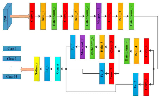
Figure 3.
MSCDN classifier architecture.
As shown in Figure 3, the MSCDN comprises seven convolutional layers, two max-pooling layers, four fully connected layers, one concat layer, and a softmax classifier. The Rectified Linear Unit (ReLU) and Batch Normalization (BN) layers are successively connected after Conv_1 to Conv_5. The aim of ReLU layer is avoid the problems of gradient explosion and gradient dispersive to further improve the efficient of gradient descent and back propagation. As for the BN layer, it is a normalized procedure for each batchsize of internal data for the purpose of standardizing the output data as the normal distribution with zero mean and unit variance, which can accelerate the convergences. The branches of Conv_6 and Conv_7 aim to reduce the depth of the output feature image from Conv_3 and Conv_4, and decrease the computational complexity. The detailed parameters of the convolution kernel for each layer and other parameters for the MSCDN structure are listed in Table 2.

Table 2.
Detailed configuration of MSCDN network architecture.
3. Experiments and Result Analysis
3.1. PolSAR Data
An experimental site, which was established by the European Space Agency (ESA), was used to evaluate the performances of the proposed method. The experimental area was an approximate 14 km × 19 km rectangular region located in the town of Indian Head (103°66′87.3″ W, 50°53′18.1″ N) in southeastern Saskatchewan, Canada. This area has 14 classes of different type of crops and an ‘unknown’ class including urban areas, transport corridors and areas of natural vegetation. The number of pixels and total area for each crop type are summarized in Table 3. The location maps from Google Earth and ground truth maps of the study area are shown in Figure 4.

Table 3.
Crop type and area statistics of study area.
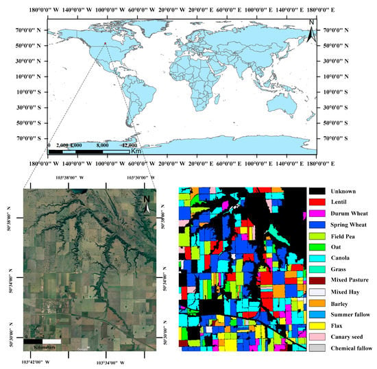
Figure 4.
Location maps and Ground truth map of the experimental site.
The experimental PolSAR data sets were simulated with Sentinel-1 system parameters from real RADARSAT-2 data by ESA before launching real Sentinel-1 systems [58]. The real RADARSAT-2 datasets were collected on 21 April, 15 May, 8 June, 2 July, 26 July, 19 August and 12 September 2009. The multi-temporal PolSAR data in these 7 periods almost covered the entire growth cycle of major crops in the experimental area from sowing to harvesting. The polarization decomposition of the single temporal PolSAR data yields 36 dimensional features. Therefore, 252 dimensional features have been acquired from 7 time-series PolSAR images.
3.2. Evaluation Criteria
For evaluating the performances of different classification methods, the recall rate, overall accuracy (OA), validation accuracy (VA) and kappa coefficient (Kappa) are considered to perform comparison.
The overall accuracy can be defined as follows
where is the total number of pixels that correctly classified, and is the total number of all pixels. Similarly, VA is the proportion of validation samples that are correctly classified to all validation samples. The recall rate can be written as follows:
where is the number of samples that are correctly classified for a certain class, is the number of samples of this class.
The kappa coefficient arises from the consistency test and is commonly used to evaluate the classification performance, it measures the consistency of the predicted output and the ground-truth. Here, we use kappa coefficients to evaluate the entire classification accuracy of the model. Unlike OA and recall rate that only involve correctly predicted samples, the kappa coefficient considered various missing and misclassified samples that located at the off-diagonal of confusion matrix. The kappa coefficient can be calculated as follows:
where is the total number of samples, is the number of crop categories, and are, respectively, the sum of the -th row and -th column elements of confusion matrix.
3.3. Results and Analysis
We now report the comparison of our method with other data compression schemes and classifiers. First, 9-dimensional compressed features were derived from the original 252-dimensional multi-temporal features using various methods, namely LLE, PCA, stacked sparse auto-encoder (S-SAE) and the proposed NC-SAE. Then, the compressed 9-dimensional features were fed into the SVM, CNN and the proposed MSCDN classifiers. The ratio of the training samples for each classifier was 1%.
3.3.1. Comparison of the Dimensionality Reduction Methods
Firstly, for the dimensionality reduction, the reconstruction error curves of SAE and NC-SAE in the training processes are shown in Figure 5. It can be seen that the reconstruction error of NC-SAE is slightly less than that of SAE. Moreover, the standard deviation within the same crop class were calculated and plotted in Figure 6A,B for different categories. The six main crops (i.e., lentil, spring wheat, field pea, canola, barley and flax) which have relatively larger cultivated areas shown in Figure 6a were chosen to evaluate the standard deviation. Meanwhile we also choose six easily confused crops shown in Figure 6b (i.e., durum wheat, oat, chemical fallow, mixed hay, barely, mixed pasture) for performance evaluation. We can see that the standard deviation of the proposed method NC-SAE is the smallest. Therefore, a better crop classification performance is expected by using the features that extracted through NC-SAE.
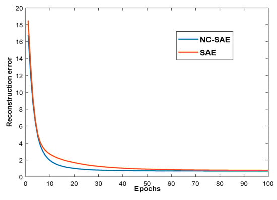
Figure 5.
The reconstruction error curves of NC-SAE and SAE.
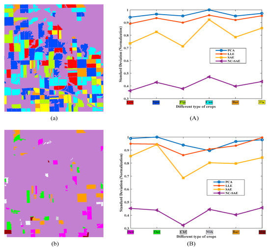
Figure 6.
The selected crops and their standard deviations of compressed data. (a) and (b) are the distribution maps of six selected crops, (a) the six crops with the largest cultivated area, (b) the six crops that are difficult to discriminate; (A) and (B) illustrate the standard deviation within the selected crops in (a) and (b), respectively.
Additionally, by using CNN classifier, the OA, VA, Kappa coefficients and CPU time performances for different dimension reduction methods are listed in Table 4, and the predicted results of the classifier and their corresponding error maps are illustrated in Figure 7. In this experiment, the size of input data for CNN classifier was set to 15 × 15.

Table 4.
Comparison of the classification performance using CNN classifier under various data compression schemes.
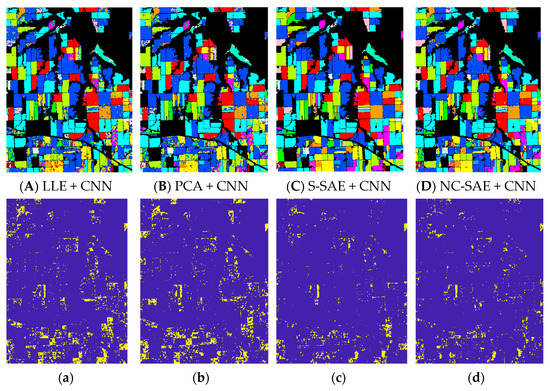
Figure 7.
Classification results and error maps: (A–D) are the classification results maps of different dimension reduction methods which are (A) LLE + CNN, (B) PCA + CNN, (C) S-SAE + CNN, (D) NC- SAE + CNN. (a–d) are the error maps of (A–D).
We can see that the dimensionality reduction methods of S-SAE and NC-SAE are both superior to PCA and LLE. For the CNN classifier, the OA and Kappa of S-SAE and NC-SAE are approximately 6~8% higher than PCA and LLE. The performances of S-SAE and NC-SAE are nearly equal. However, keep in mind that these two neural networks have different structures. The proposed NC-SAE is a single-layer network, while the S-SAE uses three auto-encoders to sequentially perform the feature compression. Comparing the CPU time that required computing the compressed features, it can be seen that NC-SAE takes almost one tenth as long as S-SAE.
3.3.2. Comparison of the Classifier with Different Classification Methods
In this section, we compare the classification performance of feeding the 9-dimensional features, which are extracted from NC-SAE, into SVM, CNN and MSCDN classifiers. The classification results and error maps for above classifiers are shown in Figure 8. It can be readily seen that the proposed MSCDN classifier behaves the best performance. In order to provide the insight into above result, we further show the OA performances of the different classifiers, along with the recall rates for each crop in Table 5. One sees that the OA performance of MSCDN is 24% and 5% higher than that of SVM and CNN. Observing the recall rate for each crop in Table 5, we see that the poorer OA for SVM and CNN is mainly due to the low recall rates of several individual crops (namely Duw: Durum Wheat, Mip: Mixed Pasture, Mih: Mixed Hay, and Chf: Chemical fallow). By further analyzing the categories of these crops in Table 3, we find that the above mentioned crops are easily confused with others because they have the same growth cycle or similar external morphologies with others. For example, Duw (Durum Wheat) is similar to Spw (Spring Wheat) in terms of external morphology, and Mip (Mixed Pasture) is more easily confused with Gra (Grass) and Mih (Mixed Hay). We conjecture that the poorer OA for SVM and CNN arise from the poorer distinguishable features that extracted by their network architectures.
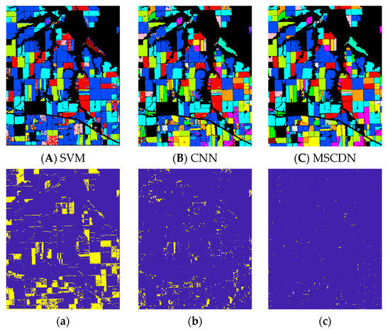
Figure 8.
Classification results for different classifiers (A) SVM, (B) CNN, (C) MSCDN; (a–c) are the error maps of (A–C).

Table 5.
The recall rates and OA of crop classification of different classifier after NC-SAE dimensional reduction.
From the above analysis, we see that the accurate classification for these easily confused crops is the key point of enhancing the overall accuracy. For deeply understanding the improvement of our MSCDN classifier, the confusion matrix of crops Duw, Mip, Mih and Chf for CNN and MSCDN are shown in Table 6. One sees that compared to CNN, MSCDN greatly improves the recall rates of these easily confused crops, whose averaged recall rate increased more than 31%. This is not surprising because MSCDN is a multi-scale neural network, the architecture of which enables to extract the features in different scales by using multiple kernels in convolution layers, and hence MSCDN is able to capture the tiny distinctions between the feature maps. Moreover, it should be pointed out that the above easily confused crops have very small samples in our crop data (only 7.3% of whole samples). Therefore, the improvement of OA performance for MSCDN will be foreseen.

Table 6.
The partial confusion matrix of crop classification for CNN and MSCDN.
3.3.3. The Performance for the Different Size of Input Sample
The size of input sample for classifiers also affects the performance for crop classification. After the compression data with NC-SAE, Table 7 gives the classification results of MSCDN classifier with different sample size, the corresponding training curves are shown in Figure 9. Firstly, we set the size of input samples for the MSCDN classifier to 15 × 15. In this scenario, slightly over fitting has been observed when training the MSCDN, which is shown in Figure 9a. This problem has been ultimately solved by increasing the size of input sample. Figure 9b shows the training curve for input samples with size of 35 × 35. We see that the over-fitting can be completely eliminated by expanding the input size. Observing Table 7, we see that the OA and Kappa increased by 4.12% and 4.98%, ultimately rise to 99.33% and 99.19%, respectively, when increasing the input size from 15 × 15 to 35 × 35, whereas when the size of input samples was expanded to 55 × 55, both OA and Kappa only raised approximately 0.3% relative to the 35 × 35, while considerable computational burden is needed. Therefore, a moderate size 35 × 35 for input samples is recommended in real applications.

Table 7.
The classification performance of MSCDN with different sample size.
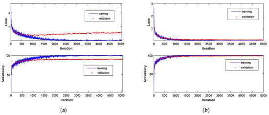
Figure 9.
Training curves with the sample size of (a) 15 × 15, (b) 35 × 35.
For the CNN classifier, the same conclusion can be made. Table 8 further demonstrates the effect of the different sizes of input sample on classification results. In addition, by comparing the results in Table 7 and Table 8, we can see that classification performance of MSCDN is always better than CNN under the same sample size.

Table 8.
The classification performance of CNN with different sample size.
3.3.4. Comparison of Overall Processing Procedures
The overall processing procedures and their performance evaluation are listed in Table 9. For classifiers of the traditional SVM, CNN and the proposed MSCDN, the data compression methods such as PCA, LLE, S-SAE and NC-SAE were used to obtain the compressed 9-dimensional features. Different from the above methods, the LSTM in Zhong et al. [25] can directly perform the classification with the 36 × 7 feature maps for a single pixel. Although the LSTM method avoids the feature compression procedure, the classification accuracy was poor. Whereas the combination of data compressor and trained classifiers can achieve remarkable crop classification performance. From Table 9, we can conclude that: (1) the combination of the proposed NC-SAE and MSCDN obtained the best performance; (2) with the expansion of the input size for CNN and MSCDN, the classification accuracy for these two classifiers has remarkably increased. However, it is worth noting that the phenomenon of over-fitting appears in NC-SAE + MSCDN for 15 × 15 sample case as shown in Figure 9, so the classification accuracy will be somewhat inferior to its competitors.

Table 9.
Classification accuracy with different methods.
4. Discussion
From an increasing number of experiments and analysis, the performance of crop classification can be improved remarkably based on multi-temporal quad-pol SAR data. Nowadays, a great number of spaceborne SAR systems launched into orbit around the Earth can enhance the revisiting period of satellite constellation and obtain a growing amount of real data, which provides a tremendous chance for multi-temporal data analysis. Additionally, the wide application of neural network in remote sensing has shown great abilities. Based on these two attentions, this paper attempted to divide two steps which are dimensional reduction based on NCSAE and then classification with MSCDN to achieve the crop classification. The summary for experimental results of Section 3 is discussed in the following.
4.1. The Effect of NC-SAE
In this paper, the NC-SAE was used to reduce the dimension of features from polarimetric decomposition. We can see that the NC-SAE has obtained the best performance compared with other methods through the experimental results in Section 3.3.1. Compared to the traditional dimension reduction methods PCA and LLE, the classification accuracy by using the NC-SAE compressed features has improved more than 6%, while nearly same accuracy compared with S-SAE. However, the S-SAE has three hidden layers with an intricate structure and more node members in each layer. The structure of NC-SAE is simple, it has only one hidden layer with 9 node members. The hyper-parameter , and of NC-SAE were set to 0.1, 2.5 and 0.45, respectively, which are directly inherited from the empirical value of S-SAE. Therefore, the NC-SAE is a computationally cheaper alternate of S-SAE.
4.2. The Effect of MSCDN Classifier
MSCDN was employed to classify the features extracted from NC-SAE dimensional reduction method, where the configuration parameters are empirically determined. The MSCDN network differs from the classical CNN network in its concatenated multi-scale features extracted by multiple kernels with different size. Though the slightly over-fitting has been observed in the training process of MSCDN when setting the input size as 15 × 15 × M, where M is the dimension of input features. This problem is readily resolved by expanding the input size to 35 × 35 × M. Moreover, the classification accuracy has been greatly improved compared to other classifiers. In general, the MSCDN classifier combined with NC-SAE feature compression method has obtained the best performance, and its overall accuracy is about 5% higher than our previous work [17].
4.3. Future Work
First of all, the phenomenon of slightly over-fitting when training the MSCDN network may be resolved by trying to put a dropout layer in MSCDN. Secondly, this study used a two stage processing networks for crop classification (features compression and subsequent classification). A more elegant one single network that implements the crop classification with multi-temporal Quad-Pol SAR data can be foreseen to further simplify the network and reduce the computation burden.
5. Conclusions
In this paper, we proposed a novel classification method, namely MSCDN, for multi-temporal PolSAR data classification. To solve the problem of the dimension disaster, firstly, we constructed a sparse auto-encoder with non-negativity constraints (NC-SAE) which has an improved sparsity to reduce the data dimension of scattering features extracted from multi-temporal PolSAR images. Meanwhile, the simulated multi-temporal Sentinel-1 data provided by the ESA and the established ground truth map for experimental site were used to evaluate the performances of the proposed methodology. Comparing the performance of classification result, we can see that the OA of MSCDN classifier is approximately 20% higher than that of traditional SVM, but only 1–2% higher than CNN. It seems that the advantage of MSCDN over the CNN classifier is somewhat trivial, but we have to note that this insignificant improvement comes from the accuracy improvement of easily confused crops with very small samples. So the overall improvement is somewhat limited. If the proposed method is applied to classify the easily confused crops with higher proportion, the remarkable improvement of OA performance will be anticipated.
Author Contributions
W.-T.Z. proposed the methodology. M.W. designed the experiments and performed the programming work. J.G. contributed extensively to the manuscript writing and revision. S.-T.L. supervised the study. All authors have read and agreed to the published version of the manuscript.
Funding
This work was supported by the National Natural Science Foundation of China (Grant No. 62071350) and the Key R & D projects of Shaanxi Province (2020GY-162).
Institutional Review Board Statement
Not applicable.
Informed Consent Statement
Not applicable.
Data Availability Statement
The data presented in this study are available in the article.
Acknowledgments
We thank the European Space Agency (ESA) for providing the simulated multi-temporal PolSAR data sets and ground truth information under the Proposal of C1F.21329: Preparation of Exploiting the S1A data for land, agriculture and forest applications.
Conflicts of Interest
The authors declare no conflict of interest.
References
- Kolotii, A.; Kussul, N.; Shelestov, A.; Skakun, S.; Yailymov, B.; Basarab, R.; Lavreniuk, M.; Oliinyk, T.; Ostapenko, V. Comparison of biophysical and satellite predictors for wheat yield forecasting in Ukraine. In Proceedings of the 2015 36th International Symposium on Remote Sensing of Environment, Berlin, Germany, 11–15 May 2015. [Google Scholar] [CrossRef] [Green Version]
- Boryan, C.; Yang, Z.; Mueller, R.; Craig, M. Monitoring US agriculture: The US Department of Agriculture, National Agricultural Statistics Service, Cropland Data Layer Program. Geocarto Int. 2011, 26, 341–358. [Google Scholar] [CrossRef]
- Kavitha, A.; Srikrishna, A.; Satyanarayana, C. Crop image classification using spherical contact distributions from remote sensing images. J. King Saud Univ. Comput. Inf. Sci. 2019. [Google Scholar] [CrossRef]
- Tyczewska, A.; Woźniak, E.; Gracz, J.; Kuczyński, J.; Twardowski, T. Towards Food Security: Current State and Future Pro-spects of Agrobiotechnology. Trends Biotechnol. 2018, 36, 1219–1229. [Google Scholar] [CrossRef] [PubMed]
- Thenkabail, P.S.; Knox, J.W.; Ozdogan, M.; Gumma, M.K.; Congalton, R.G.; Wu, Z.T.; Milesi, C.; Finkral, A.; Marshall, M.; Mariotto, I.; et al. Assessing future risks to agricultural productivity, water resources and food security: How can remote sensing help? Photogramm. Eng. Remote Sens. 2016, 82, 773–782. [Google Scholar]
- Orynbaikyzy, A.; Gessner, U.; Conrad, C. Crop type classification using a combination of optical and radar remote sensing data: A review. Int. J. Remote. Sens. 2019, 40, 6553–6595. [Google Scholar] [CrossRef]
- Wang, Y.; Xu, X.; Huang, L.; Yang, G.; Fan, L.; Wei, P.; Chen, G. An Improved CASA Model for Estimating Winter Wheat Yield from Remote Sensing Images. Remote Sens. 2019, 11, 1088. [Google Scholar] [CrossRef] [Green Version]
- Xiao, J.; Xu, L. Monitoring impact of heavy metal on wheat leaves from sewage irrigation by hyperspectral remote sensing. In Proceedings of the 2010 Second IITA International Conference on Geoscience and Remote Sensing, Qingdao, China, 28–31 August 2010; Volume 1, pp. 298–301. [Google Scholar]
- Kussul, N.; Lavreniuk, M.; Skakun, S.; Shelestov, A. Deep Learning Classification of Land Cover and Crop Types Using Remote Sensing Data. IEEE Geosci. Remote Sens. Lett. 2017, 14, 778–782. [Google Scholar] [CrossRef]
- Zhang, S.; Lei, Y.; Wang, L.; Li, H.; Zhao, H. Crop classification using MODIS NDVI data denoised by wavelet: A case study in Hebei Plain, China. Chin. Geogr. Sci. 2011, 21, 322–333. [Google Scholar] [CrossRef]
- Tatsumi, K.; Yamashiki, Y.; Torres, M.A.C.; Taipe, C.L.R. Crop classification of upland fields using Random forest of time-series Landsat 7 ETM + data. Comput. Electron. Agric. 2015, 115, 171–179. [Google Scholar] [CrossRef]
- Li, Y.; Chen, Y.; Liu, G.; Jiao, L. A Novel Deep Fully Convolutional Network for PolSAR Image Classification. Remote Sens. 2018, 10, 1984. [Google Scholar] [CrossRef] [Green Version]
- Sabry, R. Terrain and Surface Modeling Using Polarimetric SAR Data Features. IEEE Trans. Geosci. Remote Sens. 2015, 54, 1170–1184. [Google Scholar] [CrossRef]
- Skriver, H.; Mattia, F.; Satalino, G.; Balenzano, A.; Pauwels, V.; Verhoest, N.E.C.; Davidson, M. Crop Classification Using Short-Revisit Multitemporal SAR Data. IEEE J. Sel. Top. Appl. Earth Obs. Remote Sens. 2011, 4, 423–431. [Google Scholar] [CrossRef]
- Jafari, M.; Maghsoudi, Y.; Zoej, M.J.V. A New Method for Land Cover Characterization and Classification of Polarimetric SAR Data Using Polarimetric Signatures. IEEE J. Sel. Top. Appl. Earth Observe. Remote Sens. 2015, 8, 3595–3607. [Google Scholar] [CrossRef]
- Li, Z.; Chen, G.; Zhang, T. Temporal Attention Networks for Multitemporal Multisensor Crop Classification. IEEE Access 2019, 7, 134677–134690. [Google Scholar] [CrossRef]
- Guo, J.; Li, H.; Ning, J.; Han, W.; Zhang, W.-T.; Zhou, Z.S. Feature Dimension Reduction Using Stacked Sparse Au-to-Encoders for Crop Classification with Multi-Temporal, Quad-Pol SAR Data. Remote Sens. 2020, 12, 321. [Google Scholar] [CrossRef] [Green Version]
- Li, H.; Zhang, C.; Zhang, S.; Atkinson, P.M. Crop classification from full-year fully-polarimetric L-band UAVSAR time-series using the Random Forest algorithm. Int. J. Appl. Earth Obs. Geoinf. 2020, 87, 102032. [Google Scholar] [CrossRef]
- Whelen, T.; Siqueira, P. Time-series classification of Sentinel-1 agricultural data over North Dakota. Remote Sens. Lett. 2018, 9, 411–420. [Google Scholar] [CrossRef]
- Veloso, A.; Mermoz, S.; Bouvet, A.; Le Toan, T.; Planells, M.; Dejoux, J.-F.; Ceschia, E. Understanding the temporal behavior of crops using Sentinel-1 and Sentinel-2-like data for agricultural applications. Remote Sens. Environ. 2017, 199, 415–426. [Google Scholar] [CrossRef]
- White, L.; Millard, K.; Banks, S.; Richardson, M.; Pasher, J.; Duffe, J. Moving to the RADARSAT constellation mission: Com-paring synthesized compact polarimetry and dual polarimetry data with fully polarimetric RADARSAT-2 data for image classification of peatlands. Remote Sens. 2017, 9, 573. [Google Scholar] [CrossRef] [Green Version]
- Mattia, F.; Satalino, G.; Balenzano, A.; D’Urso, G.; Capodici, F.; Iacobellis, V.; Milella, P.; Gioia, A.; Rinaldi, M.; Ruggieri, S.; et al. Time series of COSMO-SkyMed data for landcover classification and surface parameter retrieval over agricultural sites. In Proceedings of the 2012 IEEE International Geoscience and Remote Sensing Symposium (IGARSS), Munich, Germany, 22–27 July 2012; pp. 6511–6514. [Google Scholar]
- Usman, M.; Liedl, R.; Shahid, M.A.; Abbas, A. Land use/land cover classification and its change detection using multi-temporal MODIS NDVI data. J. Geogr. Sci. 2015, 25, 1479–1506. [Google Scholar] [CrossRef]
- Zhang, X.-W.; Liu, J.-F.; Qin, Z.; Qin, F. Winter wheat identification by integrating spectral and temporal information derived from multi-resolution remote sensing data. J. Integr. Agric. 2019, 18, 2628–2643. [Google Scholar] [CrossRef]
- Zhong, L.H.; Hu, L.; Zhou, H. Deep learning based multi-temporal crop classification. Remote Sens. Environ. 2019, 221, 430–443. [Google Scholar] [CrossRef]
- Doualk, A. Application of Statistical Methods and GIS for Downscaling and Mapping Crop Statistics Using Hypertemporal Remote Sensing. J. Stat. Sci. Appl. 2014, 2, 93–101. [Google Scholar]
- Lee, J.S.; Grunes, M.R.; Kwok, R. Classification of multi-look polarimetric SAR imagery based on complex Wishart distribu-tion. Int. J. Remote Sens. 1994, 15, 2299–2311. [Google Scholar] [CrossRef]
- Maghsoudi, Y.; Collins, M.; Leckie, D.G. Polarimetric classification of Boreal forest using nonparametric feature selection and multiple classifiers. Int. J. Appl. Earth Obs. Geoinf. 2012, 19, 139–150. [Google Scholar] [CrossRef]
- Demirci, S.; Kirik, O.; Ozdemir, C. Interpretation and Analysis of Target Scattering From Fully-Polarized ISAR Images Using Pauli Decomposition Scheme for Target Recognition. IEEE Access 2020, 8, 155926–155938. [Google Scholar] [CrossRef]
- Nurtyawan, R.; Saepuloh, A.; Harto, A.B.; Wikantika, K.; Kondoh, A. Satellite Imagery for Classification of Rice Growth Phase Using Freeman Decomposition in Indramayu, West Java, Indonesia. HAYATI J. Biosci. 2018, 25, 126–137. [Google Scholar]
- Cloude, S.; Pottier, E. A review of target decomposition theorems in radar polarimetry. IEEE Trans. Geosci. Remote Sens. 1996, 34, 498–518. [Google Scholar] [CrossRef]
- Freeman, A.; Durden, S. A three-component scattering model for polarimetric SAR data. IEEE Trans. Geosci. Remote Sens. 1998, 36, 963–973. [Google Scholar] [CrossRef] [Green Version]
- Yamaguchi, Y.; Moriyama, T.; Ishido, M.; Yamada, H. Four-component scattering model for polarimetric SAR image decom-position. IEEE Trans. Geosci. Remote Sens. 2005, 43, 1699–1706. [Google Scholar] [CrossRef]
- Cloude, S.; Pottier, E. An entropy based classification scheme for land applications of polarimetric SAR. IEEE Trans. Geosci. Remote Sens. 1997, 35, 68–78. [Google Scholar] [CrossRef]
- Huynen, J.R. Phenomenological Theory of Radar Targets; Technical University: Delft, The Netherlands, 1978; pp. 653–712. [Google Scholar]
- Wen, Y.; Shang, S.; Rahman, K.U. Pre-Constrained Machine Learning Method for Multi-Year Mapping of Three Major Crops in a Large Irrigation District. Remote Sens. 2019, 11, 242. [Google Scholar] [CrossRef] [Green Version]
- Son, N.T.; Chen, C.F.; Chen, C.R.; Minh, V.Q. Assessment of Sentinel-1A data for rice crop classification using random for-ests and support vector machines. Geocarto Int. 2018, 33, 587–601. [Google Scholar]
- Picon, A.; Seitz, M.; Alvarez-Gila, A.; Mohnke, P.; Ortiz-Barredo, A.; Echazarra, J. Crop conditional Convolutional Neural Networks for massive multi-crop plant disease classification over cell phone acquired images taken on real field conditions. Comput. Electron. Agric. 2019, 167, 105093. [Google Scholar] [CrossRef]
- Zeyada, H.H.; Ezz, M.; Nasr, A.; Shokr, M.; Harb, H.M. Evaluation of the discrimination capability of full polarimetric SAR data for crop classification. Int. J. Remote Sens. 2016, 37, 2585–2603. [Google Scholar] [CrossRef]
- Zhou, Y.; Luo, J.; Feng, L.; Yang, Y.; Chen, Y.; Wu, W. Long-short-term-memory-based crop classification using high-resolution optical images and multi-temporal SAR data. GIScience Remote Sens. 2019, 56, 1170–1191. [Google Scholar] [CrossRef]
- Yang, C.; Hou, B.; Ren, B.; Hu, Y.; Jiao, L. CNN-Based Polarimetric Decomposition Feature Selection for PolSAR Image Clas-sification. IEEE Trans. Geosci. Remote Sens. 2019, 57, 8796–8812. [Google Scholar] [CrossRef]
- Guo, J.; Wei, P.; Liu, J.; Jin, B.; Su, B.; Zhou, Z. Crop Classification Based on Differential Characteristics of H/α Scattering Pa-rameters for Multitemporal Quad- and Dual-Polarization SAR Images. IEEE Trans. Geosci. Remote Sens. 2018, 56, 6111–6123. [Google Scholar] [CrossRef]
- Ustuner, M.; Balik Sanli, F. Polarimetric Target Decompositions and Light Gradient Boosting Machine for Crop Classification: A Comparative Evaluation. ISPRS Int. J. Geo-Inf. 2019, 8, 97. [Google Scholar] [CrossRef] [Green Version]
- Chen, D.; Peethambaran, J.; Zhang, Z. A supervoxel-based vegetation classification via decomposition and modelling of full-waveform airborne laser scanning data. Int. J. Remote Sens. 2018, 39, 2937–2968. [Google Scholar] [CrossRef]
- Jolliffe, I.T. Principal Component Analysis; Springer: Heidelberg/Berlin, Germany, 2002; pp. 1094–1096. [Google Scholar]
- Min, X.P.; Wang, H.; Yang, Z.W.; Ge, S.X.; Zhang, J.; Shao, N.X. Relevant Component Locally Linear Embedding Dimension-ality Reduction for Gene Expression Data Analysis. Metall. Min. Ind. 2015, 4, 186–194. [Google Scholar]
- Báscones, D.; González, C.; Mozos, D. Hyperspectral Image Compression Using Vector Quantization, PCA and JPEG2000. Remote Sens. 2018, 10, 907. [Google Scholar] [CrossRef] [Green Version]
- Bartlett, M.S.; Movellan, J.R.; Sejnowski, T.J. Face recognition by independent component analysis. IEEE Trans. Neural Netw. 2002, 13, 1450–1464. [Google Scholar] [CrossRef] [PubMed]
- Dehghanpoor, G.; Frachetti, M.; Juba, B. A Tensor Decomposition Method for Unsupervised Feature Learning on Satellite Imagery. In Proceedings of the IGARSS 2020—2020 IEEE International Geoscience and Remote Sensing Symposium, Waikoloa, HI, USA, 26 September–2 October 2020; pp. 1679–1682. [Google Scholar] [CrossRef]
- Ren, J.; Yu, X.; Hao, B. Classification of landsat TM image based on non negative matrix factorization. In Proceedings of the 2007 IEEE International Geoscience and Remote Sensing Symposium, Barcelona, Spain, 23–28 July 2007; pp. 405–408. [Google Scholar] [CrossRef]
- Roweis, S.T.; Saul, L.K. Nonlinear Dimensionality Reduction by Locally Linear Embedding. Science 2000, 290, 2323–2326. [Google Scholar] [CrossRef] [Green Version]
- Chen, S.-W.; Tao, C.-S. PolSAR Image Classification Using Polarimetric-Feature-Driven Deep Convolutional Neural Network. IEEE Geosci. Remote Sens. Lett. 2018, 15, 627–631. [Google Scholar] [CrossRef]
- Xie, G.-S.; Zhang, X.-Y.; Liu, C.-L. Efficient Feature Coding Based on Auto-encoder Network for Image Classification. In Proceedings of the Asian Conference on Computer Vision—ACCV 2014, Singapore, 16 April 2015; pp. 628–642. [Google Scholar]
- Kim, H.; Hirose, A. Unsupervised Fine Land Classification Using Quaternion Autoencoder-Based Polarization Feature Extraction and Self-Organizing Mapping. IEEE Trans. Geosci. Remote Sens. 2017, 56, 1839–1851. [Google Scholar] [CrossRef]
- Ren, K.; Ye, H.; Gu, G.; Chen, Q. Pulses Classification Based on Sparse Auto-Encoders Neural Networks. IEEE Access 2019, 7, 92651–92660. [Google Scholar] [CrossRef]
- Babajide, O.A.; Ayinde, E.H.; Jacek, M.Z. Visualizing and Understanding Nonnegativity Constrained Sparse Autoencoder in Deep Learning. In Proceedings of the International Conference on Artificial Intelligence and Soft Computing, Zakopane, Poland, 29 May 2016; pp. 3–14. [Google Scholar]
- Huang, L.; Xia, W.; Zhang, B.; Qiu, B.; Gao, X. MSFCN-multiple supervised fully convolutional networks for the osteosar-coma segmentation of CT images. Comput. Methods Progr. Biomed. 2017, 143, 67–74. [Google Scholar] [CrossRef]
- Caves, R.; Davidson, G.; Padda, J.; Ma, A. AgriSAR 2009 Final Report: Vol 1 Executive Summary, Data Acquisition, Data Simulation; Tech. Rep. 22689/09; ESA: Paris, France, 2011. [Google Scholar]
Publisher’s Note: MDPI stays neutral with regard to jurisdictional claims in published maps and institutional affiliations. |
© 2021 by the authors. Licensee MDPI, Basel, Switzerland. This article is an open access article distributed under the terms and conditions of the Creative Commons Attribution (CC BY) license (https://creativecommons.org/licenses/by/4.0/).


