
Performance Evaluation of Four Ocean Reflectance Model


Abstract
:1. Introduction
2. Theoretical Background
2.1. Relationship between and
2.1.1. Relationship between and
2.1.2. Relationship between and
2.2. . and Model
2.2.1. MM01 Model
2.2.2. MG07 Model
2.2.3. MO14 Model
2.2.4. Hydrolight LUTs
3. Data and Method
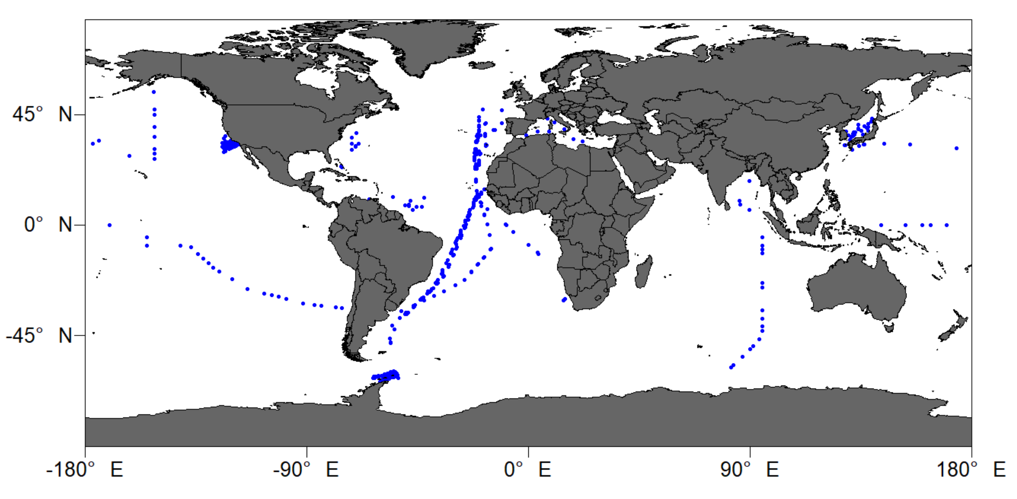
3.1. NOMAD Data Set
3.2. SCS Data Set
3.3. Statistical Method
4. Results and Discussion
4.1. Difference between the Four ORM Models
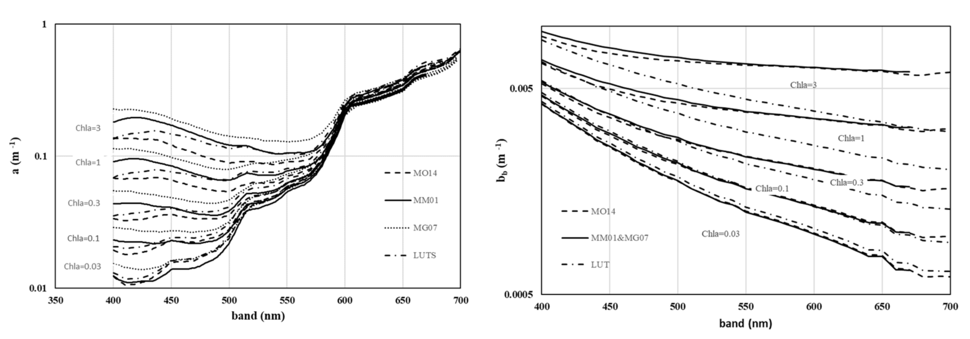
4.1.1. Difference between and of the Four ORM Models
4.1.2. Difference between the Values of the Four ORM Models
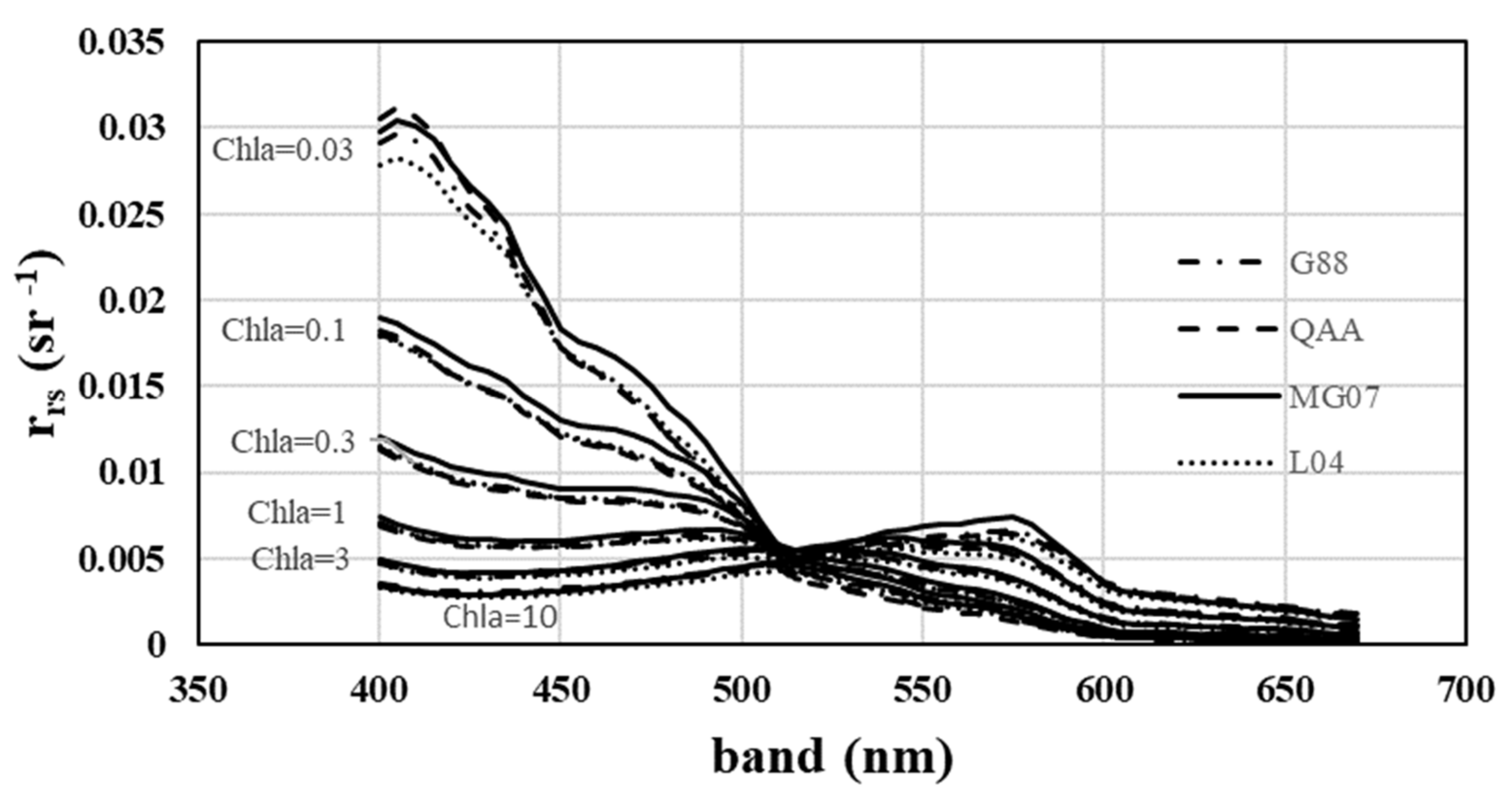
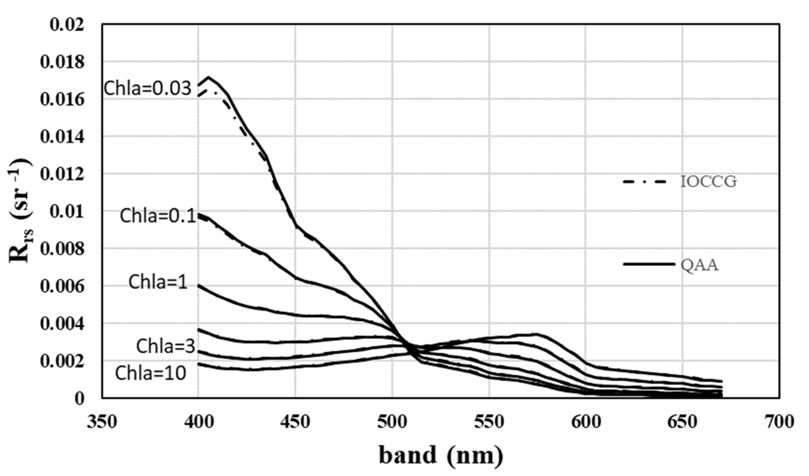
4.1.3. Relationship between and
4.1.4. Difference between of the Four ORM Models
4.2. Global and SCS Performances of the Four Models
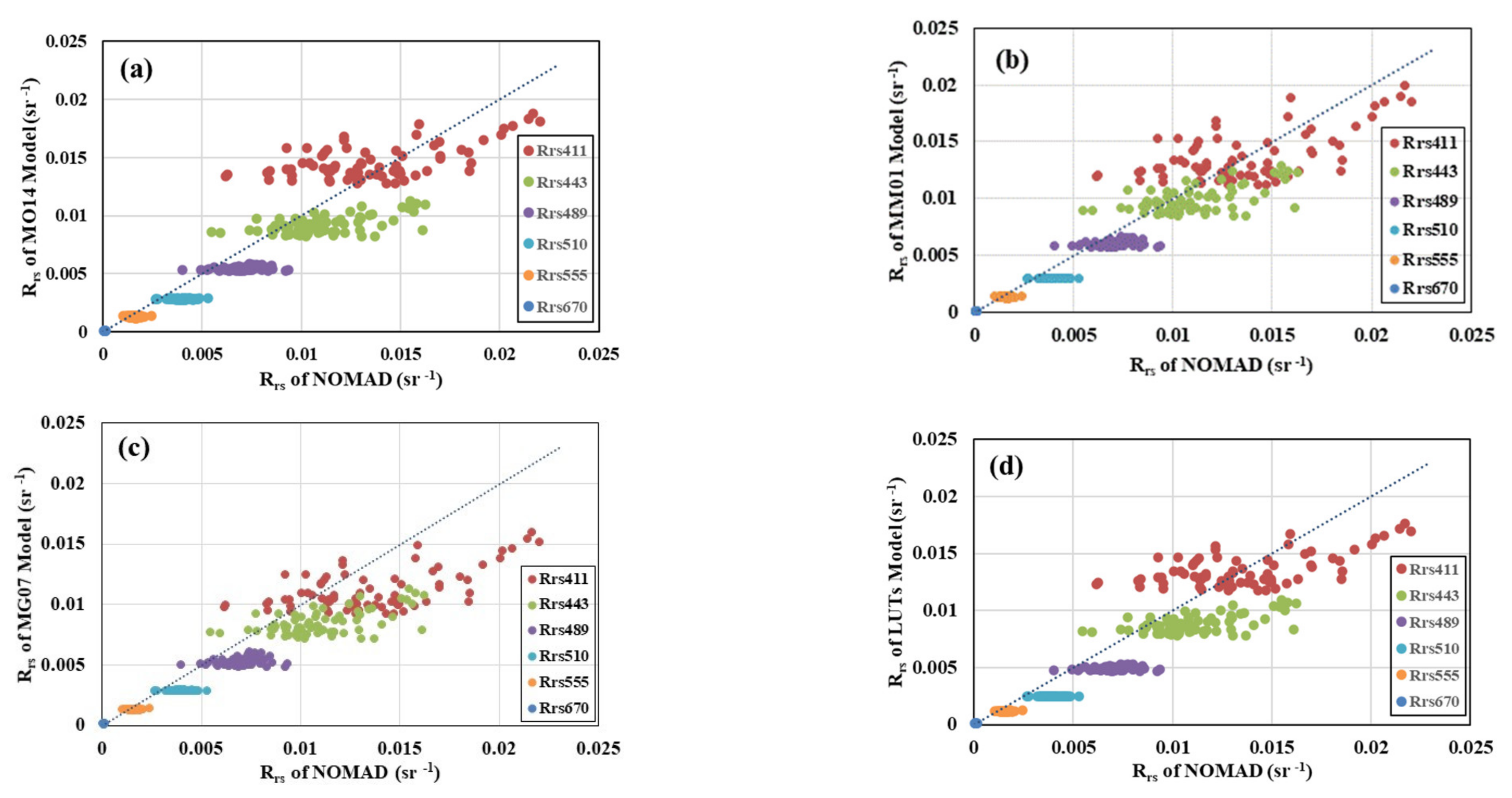
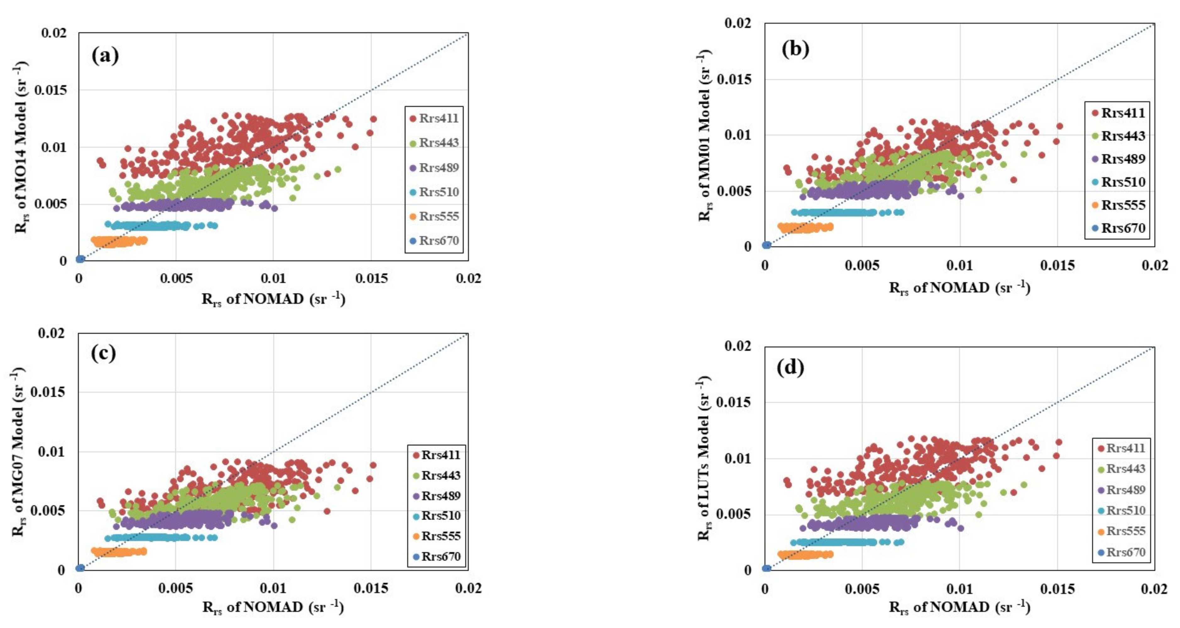
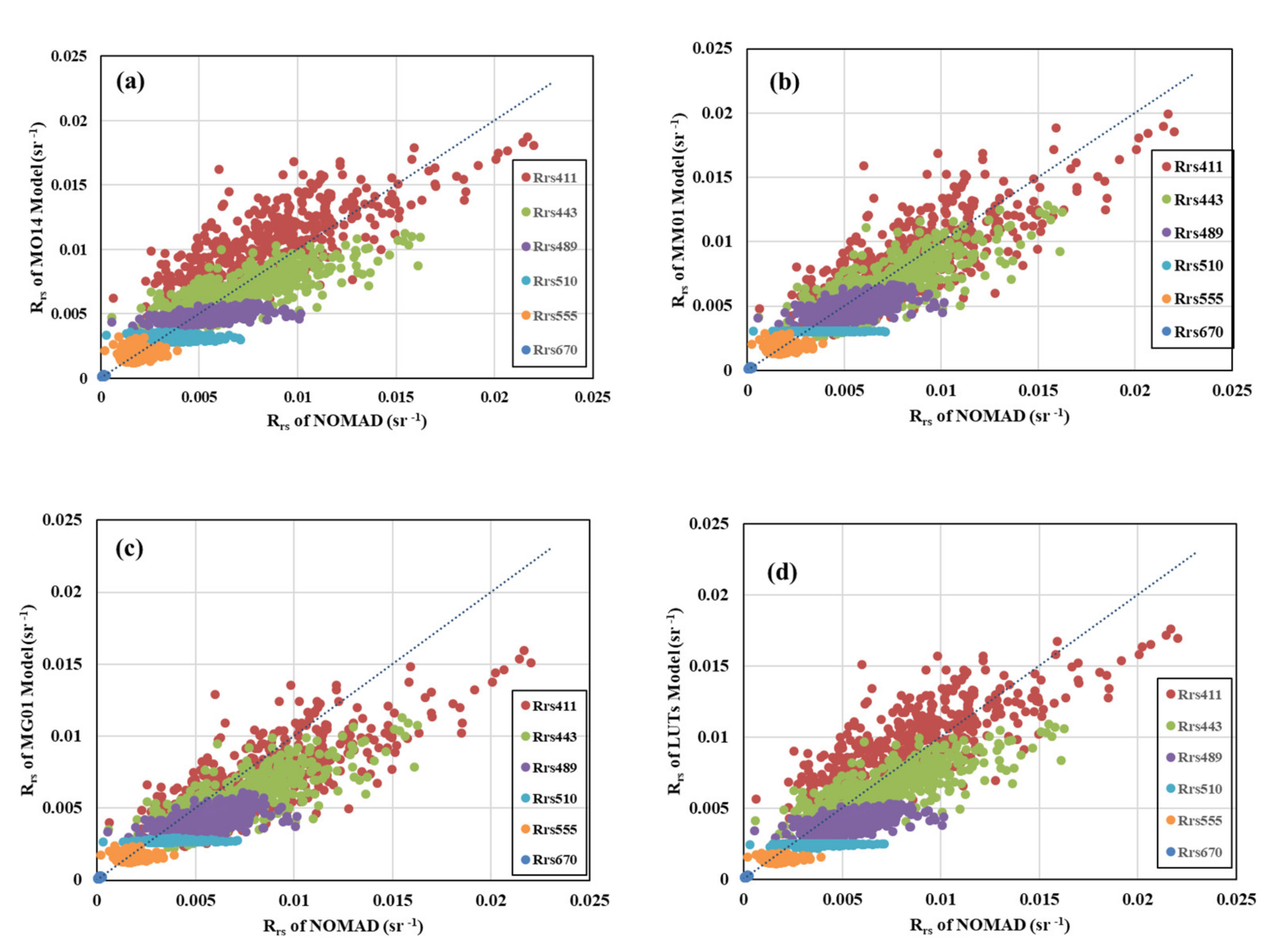
4.2.1. Global Performance of the Four ORM Models
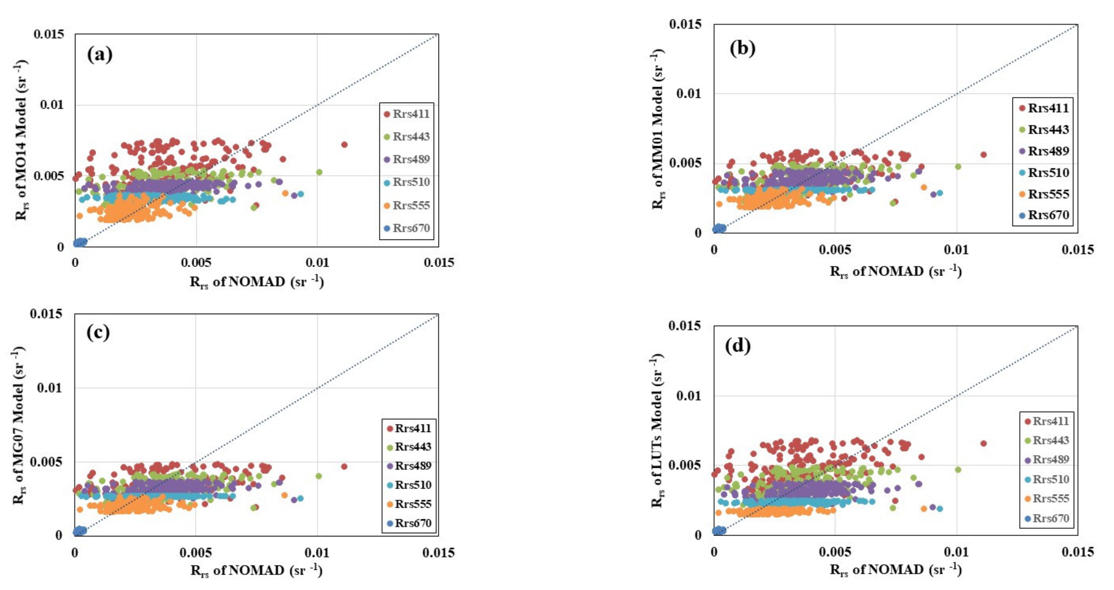
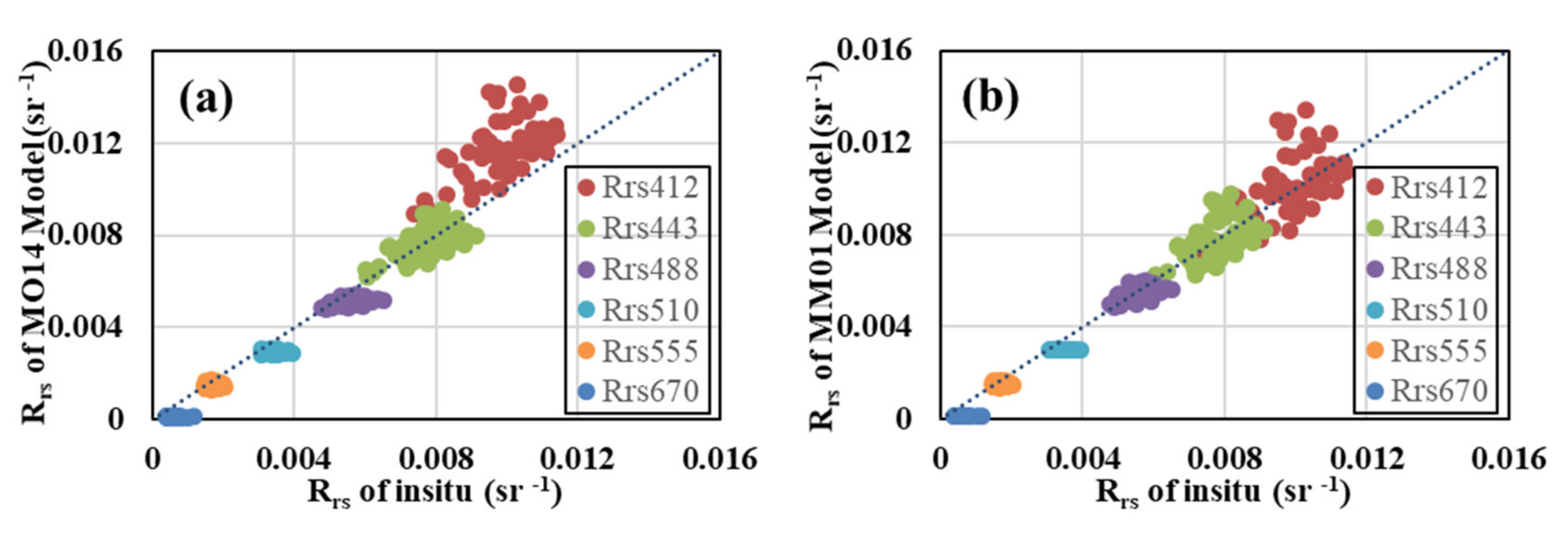
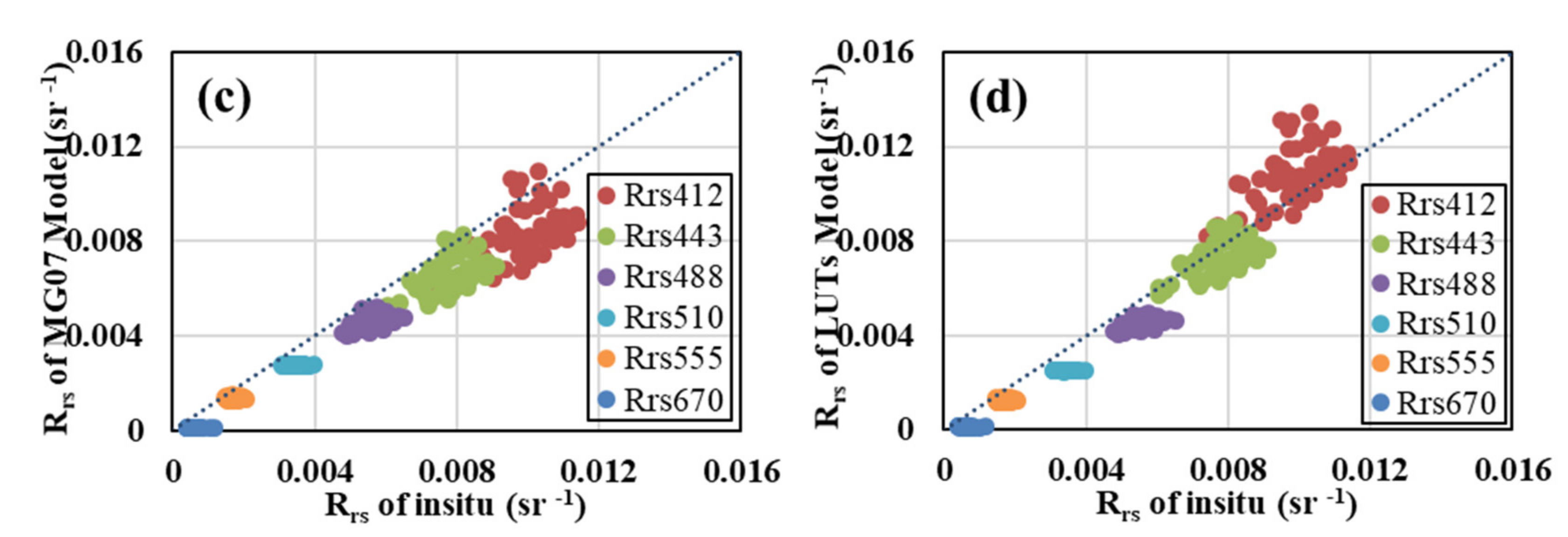
4.2.2. SCS Performance of the Four ORM Models
4.2.3. Performance of the Four Models at Different Chlorophyll Concentrations
4.3. Comparison of the Chlorophyll Algorithm and ORM Models
5. Conclusions
- For the relationship between and , the four ORM models were similar at high Chla concentrations. The differences between the four ORMs increased when the Chla concentration decreased.
- In the model of the absorption coefficient, the differences between the four ORM models were large, and MG07 was overestimated compared to the others. In the backscattering coefficients model, the differences between the four ORM models were small, and LUTs underestimated the others, where the Chla concentration was high.
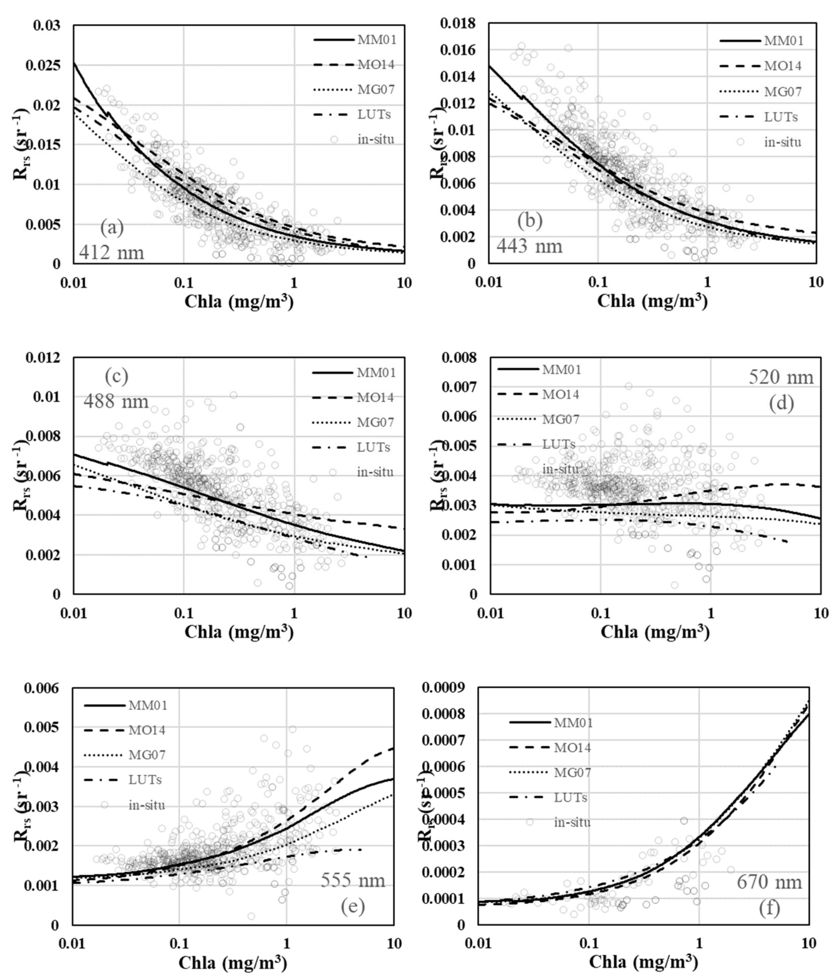
- Analysis of four ORM models and in situ match-ups of remote-sensing reflectance data showed that the model-derived values were less than those of the in situ data. The highest uncertainty was observed at 670 nm, and the APDs of the four ORM models were less than 30% globally and 20% in the SCS. The APD of MM01 was similar or better than 20% globally and in the SCS. The global and SCS performances of MM01 were better than those of the other models.
- The inversion effects of the models at different chlorophyll concentrations showed that the four models performed best when the chlorophyll concentration was less than 0.07 mg m−3, and chlorophyll concentration was between 0.07 and 0.3 mg m−3, and performance was poor when the chlorophyll concentration was greater than 0.3 mg m−3.
- The applicability of the four ORM models to the chlorophyll algorithm was compared, and the chlorophyll algorithm was analyzed using on-site spectrum measurements. The MM01 model performed best among all models; the RPD was below 3%, and the APD was below 10%. The performance of the on-site data for the algorithm was worse than that of all models, and the data dispersion was higher.
Author Contributions
Funding
Acknowledgments
Conflicts of Interest
Appendix A

| Model | |||||||
|---|---|---|---|---|---|---|---|
| MO14 | BIAS (sr−1) | 0.00101 | −0.00189 | −0.00152 | −0.00105 | −0.00025 | −0.00001 |
| RPD (%) | 13.82 | −14.10 | −20.54 | −25.84 | −14.57 | −1.93 | |
| APD (%) | 22.70 | 18.83 | 21.68 | 26.27 | 16.78 | 17.30 | |
| MM01 | BIAS (sr−1) | 0.00006 | −0.00119 | −0.00090 | −0.00088 | −0.00020 | 0.00001 |
| RPD (%) | 5.65 | −7.81 | −11.63 | −21.53 | −10.96 | 7.62 | |
| APD (%) | 20.23 | 15.69 | 14.39 | 22.40 | 14.28 | 20.17 | |
| MG07 | BIAS (sr−1) | −0.00248 | −0.00265 | −0.00172 | −0.00105 | −0.00027 | 0.00001 |
| RPD (%) | −13.87 | −21.55 | −23.59 | −25.89 | −15.67 | 8.45 | |
| APD (%) | 22.19 | 24.06 | 24.31 | 26.22 | 17.27 | 19.30 | |
| LUTs | BIAS (sr−1) | −0.00007 | −0.00224 | −0.00202 | −0.00140 | −0.00038 | 0.00001 |
| RPD (%) | 5.39 | −17.43 | −27.93 | −34.95 | −22.86 | 18.35 | |
| APD (%) | 20.37 | 21.02 | 28.46 | 34.95 | 23.46 | 24.44 | |
| Model | |||||||
|---|---|---|---|---|---|---|---|
| MO14 | BIAS (sr−1) | 0.00205 | −0.00020 | −0.00064 | −0.00064 | −0.00006 | 0.00003 |
| RPD (%) | 45.90 | 7.16 | −5.78 | −13.19 | 0.46 | 45.15 | |
| APD (%) | 49.24 | 24.54 | 20.55 | 21.00 | 15.45 | 49.38 | |
| MM01 | BIAS (sr−1) | 0.00032 | −0.00038 | −0.00046 | −0.00063 | −0.00005 | 0.00004 |
| RPD (%) | 19.54 | 3.62 | −2.68 | −13.09 | 1.04 | 57.03 | |
| APD (%) | 33.28 | 23.43 | 18.74 | 20.35 | 15.18 | 59.29 | |
| MG07 | BIAS (sr−1) | −0.00115 | −0.00140 | −0.00132 | −0.00092 | −0.00021 | 0.00004 |
| RPD (%) | −1.70 | −12.56 | −19.10 | −21.55 | −8.88 | 58.48 | |
| APD (%) | 30.97 | 27.10 | 25.84 | 25.39 | 16.24 | 60.62 | |
| LUTs | BIAS (sr−1) | 0.00121 | −0.00067 | −0.00130 | −0.00117 | −0.00034 | 0.00006 |
| RPD (%) | 33.40 | −0.65 | −18.68 | −28.52 | −16.44 | 75.29 | |
| APD (%) | 40.37 | 24.23 | 25.83 | 30.81 | 20.41 | 76.24 | |
| Model | ||||||
|---|---|---|---|---|---|---|
| MO14 | BIAS (sr−1) | 0.00170 | 0.00073 | 0.00056 | 0.00021 | 0.00020 |
| RPD (%) | 229.39 | 80.96 | 49.75 | 33.38 | 26.50 | |
| APD (%) | 234.39 | 90.69 | 60.21 | 48.17 | 39.12 | |
| MM01 | BIAS (sr−1) | 0.00046 | 0.00016 | 0.00013 | −0.00016 | 0.00004 |
| RPD (%) | 151.66 | 54.94 | 33.40 | 18.71 | 18.73 | |
| APD (%) | 168.93 | 73.73 | 50.16 | 41.50 | 34.73 | |
| MG07 | BIAS (sr−1) | −0.00023 | −0.00037 | −0.00050 | −0.00056 | −0.00031 |
| RPD (%) | 110.50 | 32.44 | 11.14 | 2.98 | 0.49 | |
| APD (%) | 140.44 | 63.58 | 43.35 | 39.46 | 29.59 | |
| LUTs | BIAS (sr−1) | 0.00117 | 0.00010 | −0.00055 | −0.00088 | −0.00059 |
| RPD (%) | 196.22 | 52.11 | 8.65 | −9.59 | −13.47 | |
| APD (%) | 204.90 | 72.30 | 42.91 | 40.96 | 31.48 | |
References
- Platt, T.; Hoepffner, N.; Stuart, V.; Brown, C. (Eds.) IOCCG Report Number 7: Why Ocean Colour? The Societal Benefits of Ocean-Colour Technology; Reports of the International Ocean-Colour Coordinating Group: Dartmouth, NS, Canada, 2008. [Google Scholar]
- Morel, A.; Huot, Y.; Gentili, B.; Werdell, P.J.; Hooker, S.B.; Franz, B.A. Examining the consistency of products derived from various ocean color sensors in open ocean (Case 1) waters in the perspective of a multi-sensor approach—Science Direct. Remote Sens. Environ. 2007, 111, 69–88. [Google Scholar] [CrossRef]
- Franz, B.A.; Bailey, S.W.; Werdell, P.J.; Mcclain, C.R. Sensor-independent approach to the vicarious calibration of satellite ocean color radiometry. Appl. Opt. 2007, 46, 5068–5082. [Google Scholar] [CrossRef] [PubMed]
- Hooker, S.B.; Bernhard, G.; Morrow, J.H.; Booth, C.R.; Comer, T.; Lind, R.N.; Quang, V. Optical Sensors for Planetary Radiant Energy (OSPREy): Calibration and Validation of Current and Next-Generation NASA Missions; NASA Technology Memo: Greenbelt, MD, USA, 2012; pp. 1–177. [Google Scholar]
- Morel, A.; Claustre, H.; Antoine, D.; Gentili, B. Natural variability of bio-optical properties in Case 1 waters: Attenuation and reflectance within the visible and near-UV spectral domains, as observed in South Pacific and Mediterranean waters. Biogeosciences 2007, 4, 913–925. [Google Scholar] [CrossRef] [Green Version]
- Lee, Z.; Carder, K.L.; Du, K. Effects of molecular and particle scatterings on the model parameter for remote-sensing reflectance. Appl. Opt. 2004, 43, 4957–4964. [Google Scholar] [CrossRef] [PubMed] [Green Version]
- Lee, Z.P. (Ed.) IOCCG Report Number 5: Remote Sensing of Inherent Optical Properties: Fundamentals, Tests of Algorithms, and Applications; Reports of the International Ocean-Colour Coordinating Group: Dartmouth, NS, Canada, 2006; pp. 1–122. [Google Scholar]
- Morel, A.; Loisel, H. Apparent optical properties of oceanic water: Dependence on the molecular scattering contribution. Appl. Opt. 1998, 37, 4765–4776. [Google Scholar] [CrossRef] [PubMed] [Green Version]
- Morel, A. Optical modeling of the upper ocean in relation to its biogenous matter content (case I waters). J. Geophys. Res. Atmos. 1988, 931, 10749–10768. [Google Scholar] [CrossRef] [Green Version]
- Morel, A.; Maritorena, S. Bio-optical properties of oceanic waters: A reappraisal. J. Geophys. Res. Ocean. 2001, 106, 7163–7180. [Google Scholar] [CrossRef] [Green Version]
- Morel, A.; Gentili, B.; Claustre, H.; Babin, M.; Bricaud, A.; Tièche, R. Optical Properties of the “Clearest” Natural Waters. Limnol. Oceanogr. 2007, 52, 217–229. [Google Scholar] [CrossRef]
- A New IOP Model for Case 1 Water. Available online: https://www.oceanopticsbook.info/view/optical-constituents-of-the-ocean/level-2/new-iop-model-case-1-water (accessed on 12 July 2021).
- Mobley, C.D.; Sundman, L.K. Hydrolight 5 Ecolight 5; Sequoia Scientific Inc.: Bellevue, WA, USA, 2008; pp. 1–95. [Google Scholar]
- Gordon, H.R.; Clark, D.K. Clear water radiances for atmospheric correction of coastal zone color scanner imagery. Appl. Opt. 1981, 20, 4175–4180. [Google Scholar] [CrossRef] [PubMed]
- An Update of the Quasi-Analytical Algorithm (QAA_v5); Technical Report: International Ocean Colour Coordinating Group (IOCCG). Available online: https://www.ioccg.org/groups/Software_OCA/QAA_v5.pdf (accessed on 12 July 2021).
- Smith, R.C.; Baker, K.S. The Bio-Optical State of Ocean Waters and Remote Sensing. Limnol. Oceanogr. 1978, 23, 247–259. [Google Scholar] [CrossRef] [Green Version]
- Pope, R.M.; Fry, E.S. Absorption spectrum (380–700 nm) of pure water. II. Integrating cavity measurements. Appl. Opt. 1997, 36, 8710–8723. [Google Scholar] [CrossRef] [PubMed]
- Mobley, C.D.; Sundman, L.K.; Davis, C.O.; Bowles, J.H.; Gleason, A. Interpretation of hyperspectral remote-sensing imagery by spectrum matching and look-up tables. Appl. Opt. 2005, 44, 3576–3592. [Google Scholar] [CrossRef] [PubMed]
- Wei, J.; Lee, Z.; Shang, S. A system to measure the data quality of spectral remote sensing reflectance of aquatic environments. J. Geophys. Res. Ocean. 2016, 121. [Google Scholar] [CrossRef]
- Mueller, J.L.; Fargion, G.S.; Mcclain, C.R. Ocean Optical Protocols for Satellite Ocean Color Sensor Vlidation; Revision 3; NASA Technology Memo: Greenbelt, MD, USA, 2003; pp. 1–137. [Google Scholar]
- Morel, A.; Mueller, J.L. Normalized Water-Leaving Radiance and Remote Sensing Reflectance: Bidirectional Reflectance and Other Factors in Ocean Optics Protocols for Satellite Ocean Color Sensor Validation; Revision 3; NASA Technology Memo: Greenbelt, MD, USA, 2002; pp. 1–137. [Google Scholar]
- Gordon, H.R.; Brown, O.B.; Evans, R.H.; Brown, J.W.; Smith, R.C.; Baker, K.S.; Clark, D.K. A semianalytic radiance model of ocean color. J. Geophys. Res. 1988, 93, 10909–10924. [Google Scholar] [CrossRef]
- Lee, Z.; Wang, Y.; Yu, X.; Shang, S.; Luis, K. Evaluation of forward reflectance models and empirical algorithms for chlorophyll concentration of stratified waters. Appl. Opt. 2020, 59, 9340–9352. [Google Scholar] [CrossRef] [PubMed]


| Model | |||||||
|---|---|---|---|---|---|---|---|
| MO14 | BIAS (sr−1) | 0.00172 | −0.00049 | −0.00070 | −0.00063 | −0.00001 | 0.00002 |
| RPD (%) | 32.05 | 1.76 | −6.03 | −11.70 | 5.05 | 31.07 | |
| APD (%) | 37.20 | 21.58 | 20.92 | 23.81 | 21.49 | 42.57 | |
| R2 | 0.7006 | 0.7144 | 0.4914 | 0.0731 | 0.2717 | 0.3964 | |
| MM01 | BIAS (sr−1) | 0.00020 | −0.00056 | −0.00053 | −0.00065 | −0.00001 | 0.00003 |
| RPD (%) | 9.70 | −1.59 | −4.10 | −12.74 | 4.71 | 42.17 | |
| APD (%) | 26.15 | 20.80 | 18.06 | 22.34 | 19.64 | 50.46 | |
| R2 | 0.7144 | 0.721 | 0.4925 | 0.0226 | 0.2686 | 0.3971 | |
| MG07 | BIAS (sr−1) | −0.00134 | −0.00159 | −0.00135 | −0.00094 | −0.00019 | 0.00003 |
| RPD (%) | −9.73 | −16.65 | −19.74 | −21.23 | −6.11 | 43.24 | |
| APD (%) | 25.50 | 25.69 | 25.74 | 27.30 | 19.02 | 50.83 | |
| R2 | 0.7144 | 0.722 | 0.4911 | 0.0641 | 0.2735 | 0.397 | |
| LUTs | BIAS (sr−1) | 0.00088 | −0.00096 | −0.00140 | −0.00121 | −0.00033 | 0.00005 |
| RPD (%) | 20.82 | −6.34 | −20.42 | −29.03 | −14.82 | 56.54 | |
| APD (%) | 30.43 | 22.16 | 26.50 | 33.42 | 22.57 | 61.57 | |
| R2 | 0.7023 | 0.7131 | 0.4856 | 0.0456 | 0.2443 | 0.3995 | |
| Model | |||||||
|---|---|---|---|---|---|---|---|
| MO14 | BIAS (sr−1) | 0.00186 | −0.00014 | −0.00054 | −0.00050 | −0.00021 | −0.00049 |
| RPD (%) | 19.23 | −1.37 | −9.14 | −14.38 | −11.85 | −80.17 | |
| APD (%) | 19.23 | 7.29 | 9.32 | 14.38 | 12.34 | 80.17 | |
| R2 | 0.327 | 0.335 | 0.1642 | 0.0033 | 0.0049 | 0.0416 | |
| MM01 | BIAS (sr−1) | 0.00021 | −0.00004 | −0.00017 | −0.00042 | −0.00018 | −0.00048 |
| RPD (%) | 2.29 | −0.24 | −2.71 | −11.97 | −9.93 | −78.56 | |
| APD (%) | 9.04 | 8.06 | 6.00 | 11.97 | 10.62 | 78.56 | |
| R2 | 0.3024 | 0.3224 | 0.1679 | 0.0029 | 0.005 | 0.0416 | |
| MG07 | BIAS (sr−1) | −0.00161 | −0.00125 | −0.00104 | −0.00066 | −0.00029 | −0.00048 |
| RPD (%) | −16.21 | −15.74 | −18.08 | −19.03 | −17.01 | −78.25 | |
| APD (%) | 17.29 | 16.16 | 18.08 | 19.03 | 17.01 | 78.25 | |
| R2 | 0.3007 | 0.3169 | 0.1577 | 0.001 | 0.005 | 0.0416 | |
| LUTs | BIAS (sr−1) | 0.00090 | −0.00056 | −0.00110 | −0.00094 | −0.00041 | −0.00046 |
| RPD (%) | 9.50 | −6.81 | −19.25 | −27.05 | −24.06 | −75.74 | |
| APD (%) | 10.35 | 9.09 | 19.25 | 27.05 | 24.06 | 75.74 | |
| R2 | 0.3234 | 0.335 | 0.1797 | 0.0679 | 0.0053 | 0.0423 | |
| Model | In Situ | |||||
|---|---|---|---|---|---|---|
| OC4 | BIAS (mg m−3) | −0.03677 | −0.03643 | −0.08382 | −0.15460 | 0.05355 |
| RPD (%) | −2.66 | 7.65 | −8.35 | −25.40 | 13.01 | |
| APD (%) | 8.13 | 17.06 | 14.35 | 25.61 | 40.13 | |
| OC3 | BIAS (mg m−3) | −0.04464 | −0.04020 | −0.08447 | −0.15132 | 0.01522 |
| RPD (%) | −2.02 | 8.94 | −7.60 | −25.04 | 10.32 | |
| APD (%) | 7.31 | 17.37 | 12.28 | 25.09 | 37.45 | |
Publisher’s Note: MDPI stays neutral with regard to jurisdictional claims in published maps and institutional affiliations. |
© 2021 by the authors. Licensee MDPI, Basel, Switzerland. This article is an open access article distributed under the terms and conditions of the Creative Commons Attribution (CC BY) license (https://creativecommons.org/licenses/by/4.0/).
Share and Cite
Li, J.; Li, T.; Song, Q.; Ma, C. Performance Evaluation of Four Ocean Reflectance Model. Remote Sens. 2021, 13, 2748. https://doi.org/10.3390/rs13142748
Li J, Li T, Song Q, Ma C. Performance Evaluation of Four Ocean Reflectance Model. Remote Sensing. 2021; 13(14):2748. https://doi.org/10.3390/rs13142748
Chicago/Turabian StyleLi, Jun, Tongji Li, Qingjun Song, and Chaofei Ma. 2021. "Performance Evaluation of Four Ocean Reflectance Model" Remote Sensing 13, no. 14: 2748. https://doi.org/10.3390/rs13142748
APA StyleLi, J., Li, T., Song, Q., & Ma, C. (2021). Performance Evaluation of Four Ocean Reflectance Model. Remote Sensing, 13(14), 2748. https://doi.org/10.3390/rs13142748