Abstract
Mapping of tree height is of great importance for management, planning, and research related to agroforestry parklands in Africa. In this paper, we investigate the potential of spotlight-mode data from the interferometric synthetic aperture radar (InSAR) satellite system TanDEM-X (TDM) for mapping of tree height in Saponé, Burkina Faso, a test site characterised by a low average canopy cover (~15%) and a mean tree height of 9.0 m. Seven TDM acquisitions from January–April 2018 are used jointly to create high-resolution (~3 m) maps of interferometric phase height and mean canopy elevation, the latter derived using a new, model-based processing approach compensating for some effects of the side-looking geometry of SAR. Compared with phase height, mean canopy elevation provides a more accurate representation of tree height variations, a better tree positioning accuracy, and better tree height estimation performance when assessed using 915 trees inventoried in situ and representing 15 different species/genera. We observe and discuss two bias effects, and we use empirical models to compensate for these effects. The best-performing model using only TDM data provides tree height estimates with a standard error (SE) of 2.8 m (31% of the average height) and a correlation coefficient of 75%. The estimation performance is further improved when TDM height data are combined with in situ measurements; this is a promising result in view of future synergies with other remote sensing techniques or ground measurement-supported monitoring of well-known trees.
1. Introduction
Parklands are an important agroforestry system widespread across the Sudano-Sahelian zone of West Africa [1,2]. In these landscapes, agriculture and livestock production systems are integrated under a sparse cover of scattered trees. Parklands have been shaped by generations of small-scale farmers aware of the multiple beneficial roles of the trees [2,3]. This is reflected in the species composition of the parklands, where the most abundant trees (e.g., Vitellaria paradoxa C. F. Gaertn., Parkia biglobosa (Jacq.) R. Br. ex G. Don, and Faidherbia albida (Delile) A. Chev.) are valued as sources of nutrition, medicine, fodder, firewood, as well as artisanal and construction material. Aside from being a subsistence resource, parkland trees are essential for ecosystem services, e.g., soil erosion prevention, nitrogen fixation, water purification, and groundwater recharge [4,5]. Moreover, they provide shade and shelter to humans and livestock. Although many local stakeholders, including farmers and agroforestry academics, recognize the importance of the parkland trees, there is a lack of landscape-scale monitoring tools that can be used for quantitative research, as well as sound and informed management [6,7]. With the increased pressure from the growing population and changing climatic conditions, and without clear conservational guidelines, these vital agroecological systems are facing an uncertain future [8,9,10].
Remote sensing methods are needed to study the landscape-scale influence of parkland trees on land productivity, hydrology, ecosystem services, and other important processes [11,12]. Optical remote sensing methods have shown promise in mapping of canopy cover in the parkland areas during the limited time windows when cloud cover is favourable [9,13,14,15,16]. These windows usually coincide with the dry season when many trees lose their leaves, so the detection of tree crowns is more difficult. Airborne laser scanning sensors have proven useful for providing high-quality information on topography, tree height, and vertical vegetation structure [17], but these systems are costly and inefficient for landscape-scale monitoring. Passive and active microwave methods have been used to measure soil moisture patterns and above ground biomass across landscapes [18,19].
One important property, which past satellite remote sensing methods have not managed to measure accurately, is the height of individual trees. Height can be used for monitoring growth and site productivity, as well as for estimating tree age, biomass, stem volume, and carbon content using allometric equations [20,21]. While other tree properties, mainly stem and crown diameter, can also be utilized for these applications, tree height is potentially easier to map and monitor with the cloud-penetrating and weather-independent interferometric radar satellites.
Across-track interferometric synthetic aperture radar (referred to as InSAR in the following text) uses radar data acquired from two slightly different positions in space to measure elevation at high vertical and spatial resolutions [22]. It has in the past given unprecedented information about the Earth, in particular the first near-global digital elevation model (DEM) acquired in February 2000 with the Shuttle Radar Topography Mission (SRTM) [23]. Since 2010, the twin-satellite TanDEM-X (TDM) system has been providing high-resolution InSAR data, which have been used to create a more accurate and fully-global DEM with a spatial resolution of 12 m and vertical accuracy better than 0.5 m [24,25].
TDM data have also been useful in the mapping of forest properties across biomes, in particular in densely forested areas with known ground topography [26,27,28,29,30,31,32,33,34]. Without topographic information, tree height estimation becomes challenging due to the lack of a suitable reference point. Although the exact topography is unknown for most parkland areas, the canopy cover is generally sparse, and tree height estimation may still be feasible with high-resolution TDM data. However, new challenges occur when mapping individual trees with high-resolution InSAR. Geometric distortions caused by the side-looking geometry introduce tree height-dependent range offsets, hindering tree positioning and distorting tree crown outlines. Additionally, the significant ground scattering and penetration into tree crowns introduce biases in tree height estimation.
The main objective of this paper is to assess the potential of high-resolution TDM InSAR data for landscape-level mapping and monitoring of tree height in a parkland landscape in Burkina Faso with unknown topography. This work is part of a larger project focusing on exploring the unknown role of trees in crop production in agroforestry parklands; as such, it aims to provide a reliable method for landscape-scale mapping and monitoring of tree height, which is a proxy of many other tree properties. In this paper, we first introduce a novel, model-based processing approach that mitigates range offset and ground scattering effects, which are especially significant when studying individual trees with high-resolution TDM data. Using seven spotlight-mode TDM acquisitions with azimuth resolution of 1.1 m, we show that the new processing approach provides a mean canopy elevation estimate that has better potential for tree height mapping than the commonly used phase height, both in terms of top-of-canopy tree height estimation and tree positioning. We also compare the results for 915 trees from 15 different species/genera and we observe and discuss two bias effects in the data: one caused by vegetation bias in the DTM, and one caused by crown shape variability across different species. Finally, we investigate the potential improvement in tree height estimation accuracy when using TDM data with empirical models, both alone and in combination with in situ data of diameter at breast height, crown diameter, and species.
2. Method
InSAR is an active, microwave remote sensing tool capable of high-resolution elevation measurements, independent of clouds and solar illumination. InSAR systems use the phase difference between two complex-valued images acquired from slightly different positions in space to measure the elevation of objects above a reference surface [22]. TanDEM-X (TDM) consists of two X-band (centre frequency: 9.65 GHz, wavelength: 3.1 cm) SAR satellites flying in a close tandem formation [35]. Because of the short wavelength and the small distance between the satellites (typically below 1000 m), the TDM DEM over vegetated areas often represents canopy height variations. However, there are several challenges associated with the estimation of vegetation height from a TDM DEM.
Firstly, information about ground topography is needed for estimation of vegetation height from an InSAR DEM [36], ideally in the form of a digital terrain model (DTM). Since most global, wall-to-wall DEMs have been acquired with either high-frequency InSAR or optical data [37], they contain vegetation bias and are not useful as ground reference in densely vegetated areas. Airborne lidar scanning (ALS) can be used in combination with InSAR data to provide accurate forest height measurements [26,28,29,32,38], but ALS data are costly to acquire and are not available for most parts of the world. Spaceborne lidar sensors, like the Global Ecosystem Dynamics Investigation (GEDI) mission from NASA [39], are a viable option for global mapping of topography, but the spatial resolution of the acquired DTMs is still relatively low (1 km in the case of GEDI).
Secondly, the elevation measured by an InSAR system is influenced by all objects within a resolution cell, which is slanted due to the side-looking geometry of SAR. Consequently, the measured elevation depends on InSAR system configuration and geometry, as well as the distribution of targets within the resolution cell. In sparsely forested areas, ground and vegetation targets can be observed within the same resolution cell. Additionally, geometric distortions prevail due to the projection of a three-dimensional scene onto a two-dimensional image plane [40].
Thirdly, the difference between the top-of-canopy tree height and the canopy elevation perceived by the radar depends on canopy density, shape, structure, phenology, and moisture, as well as radar polarisation and incidence angle. The relationship between elevation measured with TDM and top-of-canopy height varies in time and with acquisitions.
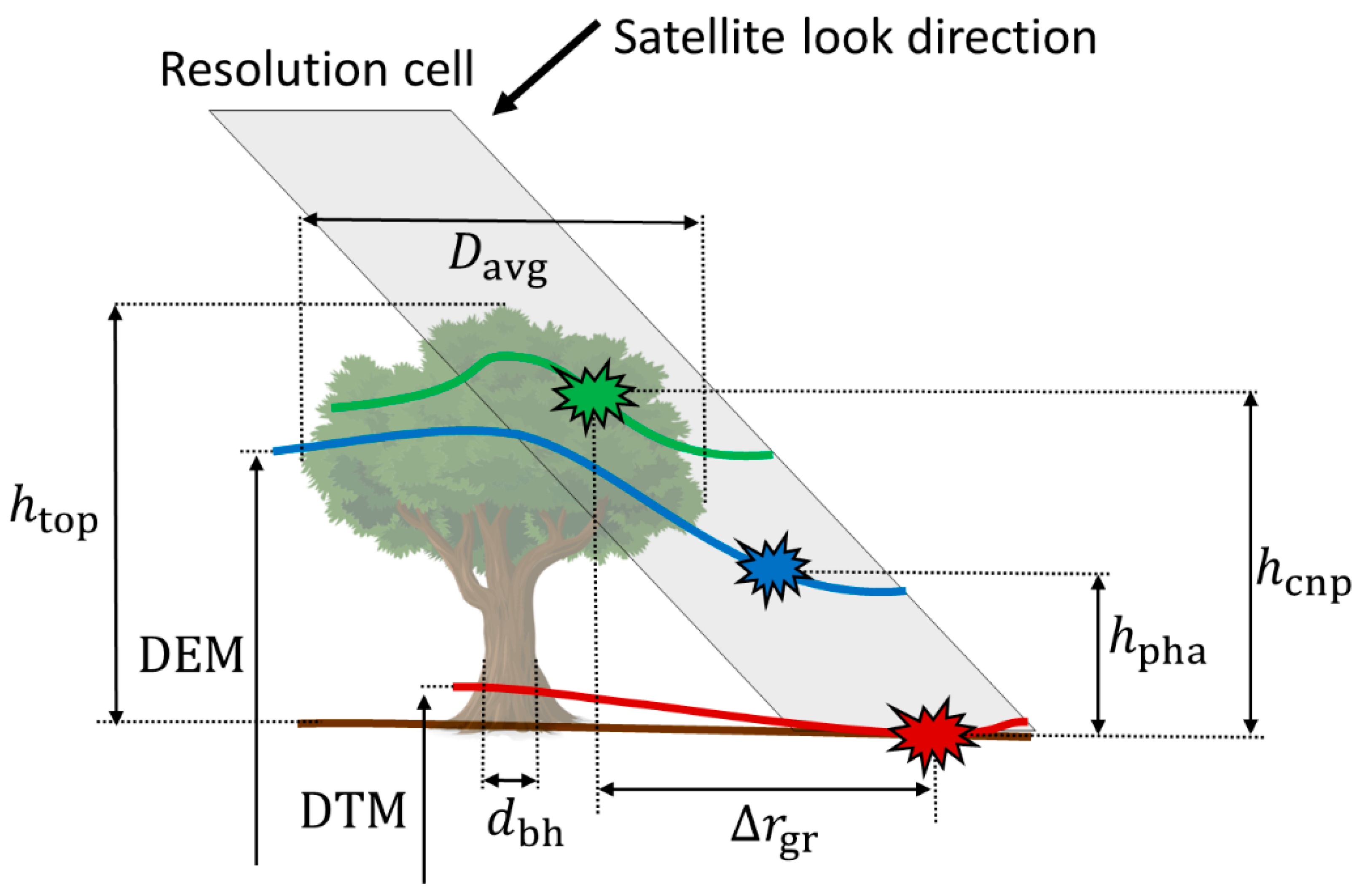
Figure 1 shows the geometry of an InSAR measurement of a single tree with top-of-canopy tree height , average tree crown diameter , and stem diameter at breast height (1.3 m) . Two InSAR quantities used in this paper are also indicated: is the phase height, i.e., the difference between the DEM and the DTM, while is the mean canopy elevation above the DTM. The slanted geometry of the InSAR measurement is also shown; as a result, ground and canopy objects within the same resolution cell are located at a ground range offset .

Figure 1.
Illustration of some quantities used in this paper. The top-of-canopy tree height is a purely geometrical quantity. Two InSAR quantities related to tree height are also shown: (1) Phase height () is the estimated difference between a digital elevation model (DEM) and a digital terrain model (DTM). (2) Mean canopy elevation ( ) is a model-based estimate of canopy height above the DTM. The ground range offset is caused by geometrical distortion due to the slanted measurement geometry of SAR. is the average diameter of the tree crown and is the stem diameter at breast height (1.3 m).
Table 1 contains a summary of different metrics (mostly height-related) used throughout this paper, including some that will be introduced later.

Table 1.
Summary of some metrics used throughout this paper.
In the next section, we define in terms of the InSAR data. Thereafter, we define the model used to compute from and coherence data, as well as the geometric correction . Finally, we discuss the relationship between , , and .
2.1. Phase Height
The main interferometric quantity is the complex correlation coefficient (), defined as [22]:
where and are two single-look complex (SLC) images acquired by an InSAR system; is the coherence, i.e., the magnitude of the complex correlation coefficient; is the interferometric phase; is a modelled interferometric phase for a reference surface; and is the expectation value operator. Coherence is a value between 0 and 1 representing the degree of similarity between and , while interferometric phase is the phase difference between and , corrected for the variability induced by the reference surface. In practical application, the expectation value in (1) is replaced by spatial averaging using a sliding window. The coherence and phase estimated using this approach are affected by well-known errors [22]. In the case of coherence, coherence overestimation occurs for low numbers of samples and/or low coherence values. In the case of interferometric phase and disregarding phase ambiguities, the estimator is unbiased, but the estimated phase has a zero-mean Gaussian error.
Assume a well-designed InSAR system, an acquisition geometry (in terms of incidence angle and distance between the two satellites) providing good sensitivity to typical vegetation heights, negligible temporal change between the two acquisitions, and adequate signal processing including common-band and wavenumber shift filtering. Furthermore, assume that in (1) represents the topographic phase modelled from a DTM. Under these assumptions, phase height can be estimated from (1) using:
where represents unwrapping, i.e., estimation of phase and removal of 2 ambiguities; and is the height-to-phase conversion factor, determining the sensitivity of the InSAR system to height variations. depends on system properties such as wavelength, separation between the satellites, and incidence angle [41]. is related to the height-of-ambiguity (HOA), i.e., the height offset corresponding to a 2 shift of the interferometric phase, according to:
Note that in (2), unwrapping is done after topographic phase () removal in (1). It is also possible to estimate by first creating a DEM and then subtracting a DTM. However, because the DEM is expected to have larger height variations than , that approach is more susceptible to phase unwrapping errors.
2.2. Mean Canopy Elevation
Volume decorrelation is a loss of coherence caused by the distribution of targets in the direction perpendicular to the image plane. Several models for volume decorrelation in vegetation have been used with TDM data in the past [26,28,29,33,42]. In this paper, we will use the two-level model (TLM) [29,43], where the scattering is assumed to originate from only two levels. It directly separates ground and canopy contributions in InSAR data and does not require multi-polarised data or allometric equations. In the TLM, volume decorrelation is modelled using two discrete levels, ground and vegetation [44]:
where is the vegetation scattering fraction and is the elevation of the vegetation level above the ground level. The vegetation scattering fraction describes the distribution of scattering between the two levels, and it depends on the canopy cover and ground-to-vegetation backscatter ratio as [44]:
In this paper, we use the multiplicative coherence model from [22,45] to estimate volume decorrelation using:
where is the complex correlation coefficient from (1) and is an estimate of signal-to-noise decorrelation, i.e., the loss of similarity due to different noise representations in the two images [45]. Note that (4) neglects all decorrelation effects other than volume and signal-to-noise decorrelation. By fitting model (3) to the measured and calibrated data from (4), estimates of and are obtained.
The estimated above contains the ground range offset described at the beginning of Section 2 and shown in Figure 1. If and are the respective easting and northing coordinates (in metres) of the measured and data, then the value of at these coordinates is assumed to represent the mean canopy elevation () at a position shifted in ground range away from the radar by . For a right-looking system (like TanDEM-X) and disregarding topographic undulations, can be estimated from (in metres) through the following interpolation:
where is the incidence angle and is the flight heading angle (see Figure 2). The factor maps to the ground range offset , while factors and project in the east and north directions, respectively.

Figure 2.
Acquisition geometry for a right-looking SAR system, with the incidence angle () and heading angle () shown together with the principal axes of a SAR acquisition. are the respective east and north coordinates of a grid cell. (a) Elevation plane; (b) ground plane.
2.3. Estimation of Tree Height
Both and provide biased estimates of due to the penetration of X-band radar signals into the canopy and residual effects of ground topography and inaccuracies in the DTM. Note that includes the ground scattering contribution, which aims to mitigate.
In this subsection, we use models to address two potential bias sources: crown shape variations and vegetation bias from the DTM. In Section 3.4 we introduce some empirical models used to compensate for these effects. Other effects, including varying canopy density, moisture, and phenology, are addressed further in Section 5.
2.3.1. Effect of Crown Shape
For the high-resolution InSAR data studied in this paper, tree crowns often occupy several grid cells. In this paper, we approximate a tree height measurement by taking the topmost pixel within the tree crown extent of the images of and . The corresponding tree height proxies are referred to as and , respectively, with the bar symbol indicating the selected topmost pixel.
Trees with the same top-of-canopy height , but with differently shaped crowns may have different values due to different distribution of canopy objects within the topmost pixel (and, indirectly also different values). This is illustrated with a geometric model in Figure 3a. The model assumes ellipsoidal tree crowns with the horizontal semiaxes both equal to and the vertical semiaxis equal to . Furthermore, we assume no penetration into the tree crown and that the resolution cell giving is centred on the tree trunk and has a width This crown shape bias can then be modelled as the maximal height difference within the resolution cell:
with the negative sign indicating underestimation of tree height.

Figure 3.
A simple geometric model is used to investigate the effect of crown shape on the observed difference between and . (a) Trees are modelled as ellipsoids and crown shape bias is the maximal height difference within a resolution cell centred on the treetop. (b) Sample modelling results for m.
Figure 3b shows expression (6) plotted against , which is an indicator of canopy shape, with lower values indicating narrow canopies and higher values indicating wide canopies. Three values for are used and m is assumed. The effect of crown shape bias is largest for shorter trees and/or trees with narrow canopies (low ). For taller trees or trees with wider canopies, the bias is typically less than −1.0 m.
2.3.2. Effect of Vegetation Bias from the DTM
Vegetation bias is the residual effect of vegetation on a digital terrain model (DTM), typically resulting in an overestimation of topographic height in vegetated areas, see Figure 4a. This, in turn, manifests itself as underestimation of tree height if a biased DTM is used as reference. In this work, we use a low-resolution InSAR DEM as a DTM. Overall, this approach provides good results in sparsely forested areas (like the parklands studied here). However, vegetation bias from the DTM may still be noticeable around tall trees with wide canopies.

Figure 4.
The effect of vegetation bias from the DTM on tree height estimation. (a) Vegetation bias is the offset between the DTM and the true ground surface, caused by vegetation objects. (b) Sample results showing the effect of vegetation bias from the DTM on tree height estimation, as modelled by TLM for ( m).
Vegetation bias from the DTM can be modelled using the TLM described in Section 2.2. We here assume that the average canopy cover within a DTM resolution cell is and the height of all trees is . Additionally, we assume that the backscattering coefficients for ground and vegetation are equal () and that there is no penetration into tree canopies. Under these assumptions, the effect of vegetation bias from the DTM is modelled by the TLM expression (3) to:
where the minus sign reflects the fact that a positive vegetation bias in the DTM causes a negative bias in the (and ).
The resulting bias effect is shown in Figure 4b, for different forest height and canopy cover values, and assuming ( m). For the studied forest area, the average tree height is about 9 m and the average canopy cover at 1 ha scale is typically 15%, so the modelled effect of vegetation bias from the DTM is −1.3 m. For some 1 ha areas centred around tall trees with wide canopies, the average height at 1 ha-scale can reach 16 m and canopy cover can reach 25%; in that case, effect of vegetation bias in the DTM can cause a bias about −3.7 m. Furthermore, if penetration into vegetation canopies and crown shapes are also considered, the vegetation bias will be less significant. It is thus expected that only for some of the largest trees, the effect of vegetation bias will be noticeable.
3. Experimental Data
3.1. Test Site
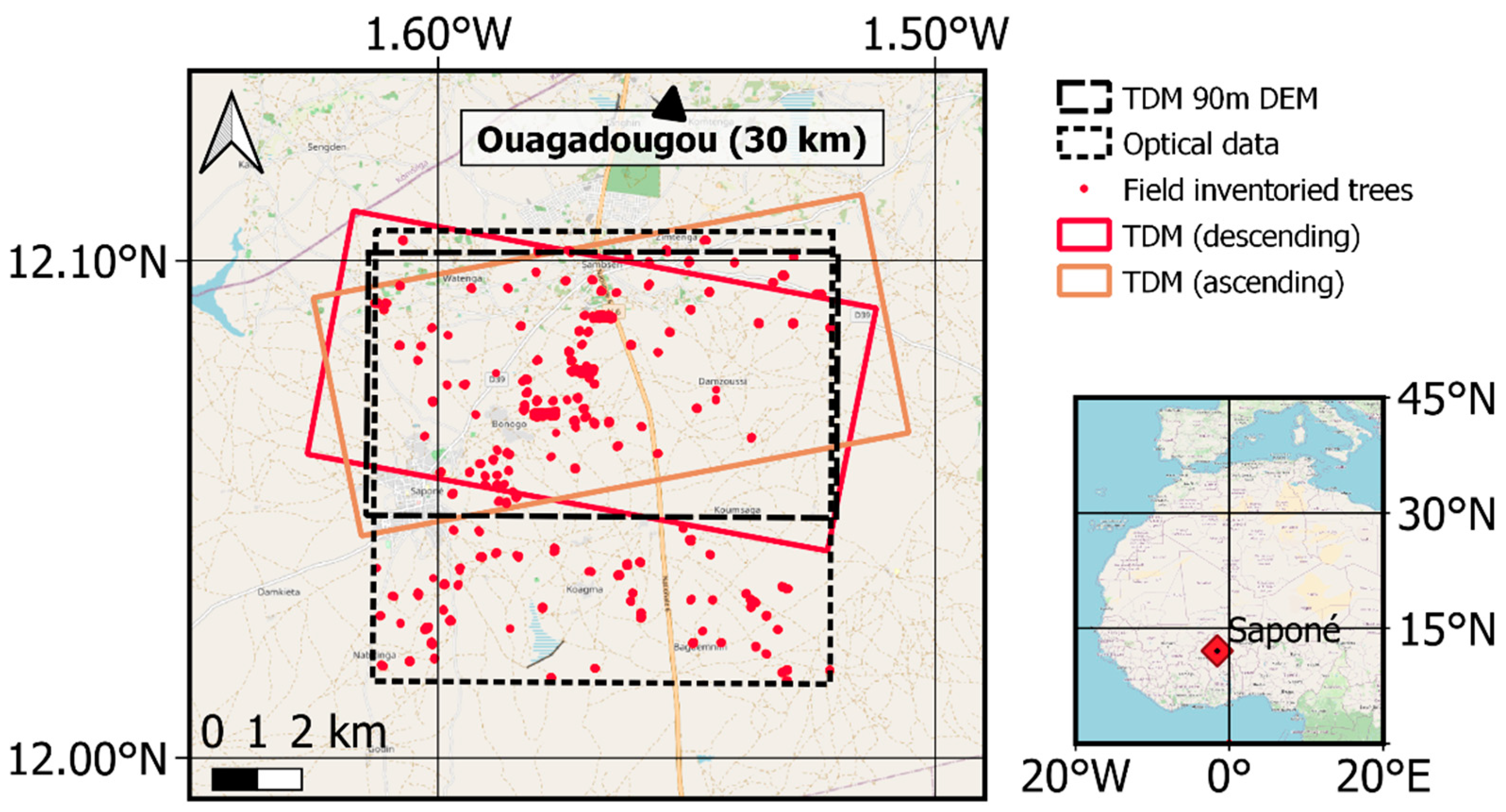
Saponé (12.08°N, 1.57°W) is a rural commune located about 30 km south from Ouagadougou, the capital of Burkina Faso (Figure 5). The test site is a 10 km × 10 km area dominated by parklands, but also featuring other land cover classes, such as patches of woodlands, small-scale plantations (Mangifera indica L., Eucalyptus camaldulensis Dehnh., and Tectona grandis L.f.), and riparian formations. The terrain is relatively flat, with altitudes varying between 293 and 363 m above sea level [46]. The climate is semi-arid, where the mean annual rainfall is around 800 mm with high inter-annual and inter-seasonal variability. The rainy season generally extends between May and October, with July and August producing the largest proportion of rainfall. The dry season features only sporadic and limited rainfall, and typically starts around November and lasts until May or June.
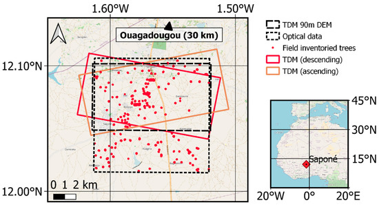
Figure 5.
Coverage of the data used in this study and location of the Saponé test site. Ouagadougou, the capital of Burkina Faso, is located about 30 km north of Saponé. The outline for optical data represents the coverage of the two high-resolution satellite images used in this study (one from WorldView-2 and one from Pléiades). Basemap: © OpenStreetMap contributors, CC-BY-SA.
The tree cover in the parklands is actively shaped by the farmers practicing naturally assisted regeneration, where favoured tree species are protected when preparing the fields before sowing [5]. Crown pruning is also practiced, to revitalise fruit production, limit shading of crops, and provide fodder [47]. Mean tree canopy cover within the test site is around 15 percent. The tree cover is dominated by traditional agroforestry species, including the native V. paradoxa, P. biglobosa, and Lannea microcarpa Engl. and K. Krause, as well as M. indica [48], native to the Indian subcontinent but often cultivated in the area. Although these species are generally considered deciduous, they are seldom leafless due to a progressive leaf replacement throughout the year [49]. Notable exceptions include L. microcarpa, which loses all its leaves early in the dry season, and F. albida, which has reverse phenology and is foliated only during the dry season.
3.2. Reference Data
Two orthorectified, high-resolution optical satellite images over Saponé were used in this study: one image acquired in December 2012 with the WorldView-2 satellite and one image acquired in October 2017 with a Pléiades satellite. Both images had a ground sampling distance of about 50 cm.
For initial geocoding of the TDM spotlight-mode data, we used the freely available, global 90 m TDM DEM [25]. We did not use the available higher-resolution TDM DEMs because we wanted to reduce vegetation bias, and the resolution of 90 m was found sufficient for initial geocoding in this relatively flat test site.
The in situ tree inventory data included three datasets collected in 2012, 2017 and 2018 (Table 1). For each dataset, trees with stem diameter at breast height (, measured at 1.3 m) ≥ 5 cm were georeferenced using a handheld Garmin Oregon 550 GPS and tree species were recorded. Top-of-canopy tree height () was measured using a Haglöf electronic clinometer from a distance between 10–20 m, depending on the line of sight. The average crown diameter () was determined by averaging two perpendicular crown diameter measurements. Positional uncertainties related to GPS accuracy were accounted for by manually matching easily identifiable trees with the high-resolution optical imagery using information on crown diameter, height, and species.
The in situ dataset from 2012 was collected between October and December within 76 plots (50 m × 50 m in dimensions), randomly distributed throughout the 100 km2 test site and equally divided between three canopy cover classes, derived using the WorldView-2 image [15,20,48]. This resulted in a total of 1125 measured trees.
The in situ dataset from 2017 was collected in October using a sampling approach where plots were randomly placed in active parkland fields identified in the Pléiades image acquired two weeks before the inventory. This dataset consisted of 637 trees distributed over the entire 100 km2 test site.
The in situ dataset from 2018 was acquired in June. Three large plots (about 500 m× 100 m in dimensions) were laid out in the central part of the test site, and a total of 321 trees were measured within these three plots. The three plots were chosen to cover areas with well-separated trees.
The three datasets were subsequently filtered to only include trees covered by all TDM acquisitions (see Section 3.3 and Figure 5). Trees that had undergone visible change (e.g., removal or significant pruning) between the December 2012 WorldView-2 image and the October 2017 Pléiades image were also excluded. The remaining trees were then sorted by species (or genus, if species could not be determined) and species/genera with less than five trees were excluded from the dataset. This resulted in a total of 915 trees left for this analysis, representing 15 different species/genera, see Table 2.

Table 2.
Summary of the in situ data from Saponé, Burkina Faso, used in this study. The second column from the left contains the number of trees fulfilling the conditions described in Section 3.2, as well as the total number of trees sampled in field.
Note that although the TDM data were acquired in early 2018, the temporal offsets between all three in situ datasets and the TDM data were ignored in this study. In particular, this concerns the dataset from 2012, which was included because it contained the largest number of in situ measured trees, allowing a more reliable statistical analysis and a more extensive study of the effect of tree species; also, it featured trees with the lowest average tree heights and crown diameters, thus improving the sampled interval of tree heights and crown diameters, see Table 2. Additionally, the growth rate for most of the tree species is low in the relevant conditions and our empirical investigations showed no noticeable effect of temporal difference between the three datasets.
3.3. TanDEM-X Data Processing
This study used a total of seven HH-polarised TDM spotlight-mode acquisitions made between January and April 2018. Three acquisitions were made from the descending orbit (flight heading around 191° relative to true north), at an incidence angle of 32 degrees (at scene centre), with HOA values between 39 and 55 metres, and with approximate ground range and azimuth resolutions at scene centre of 2.1 and 1.1 metres, respectively. The remaining four acquisitions were made from the ascending orbit (flight heading about 349°), at an incidence angle of about 25 degrees, with HOAs between 49 and 87 metres, and with ground range and azimuth resolutions of 2.8 and 1.1 metres, respectively. Table 3 contains a summary of the acquisition parameters, together with air temperatures recorded at Ouagadougou Airport at the time of acquisition [50]. All acquisitions were made during the dry season and no precipitation was recorded at Ouagadougou Airport during the 72 h prior to any of the seven acquisitions [50]. Figure 5 shows the approximate outlines of the ascending and descending acquisitions. The joint area covered by all seven acquisitions was 4200 hectares.

Table 3.
Summary of the SAR acquisitions over Saponé, Burkina Faso used in this study. “No” refers to the relative orbit number, “Dir” refers to orbit direction (“dsc” is descending and “asc” is ascending), and are the flight heading and incidence angles, respectively (see Figure 2), “Pol” refers to polarisation, “Res” refers to resolution (“grg” is ground range and “az” is azimuth), and “Temp” refers to temperature.
All acquisitions from the same orbit were co-registered to one single master image using the GAMMA software package [51]. The remaining processing was then conducted using Python scripts based on [52]. Fine-resolution interferograms (images of ) were formed using a sliding 1 × 2 window (range × azimuth), giving an approximate azimuth resolution of 2.2 m and ground range resolutions of 2.1 m for the descending data and 2.8 m for the ascending data. For coherence, a 5 × 5 window was used to reduce bias in coherence estimation [22].
Next, orbit state vectors and the free global 90 m TDM DEM [25] were used to create simulated DEM phase images, which were then subtracted from the fine-resolution interferograms, providing flattened interferograms. These were subsequently filtered using a sliding 45 × 45 averaging window, producing flattened interferograms with an approximate resolution of 100 m. A digital terrain model (DTM) was created from these coarse interferograms by unwrapping and scaling to height, then averaging across all seven acquisitions, and finally adding back to the 90 m TDM DEM. Phase height ) images were created by first subtracting the coarse-resolution flattened interferograms from the fine-resolution flattened interferograms, and then unwrapping and scaling to height.
The seven phase height images obtained were then geocoded and averaged into two images: for the ascending orbit and for the descending orbit. Then, spatial cross-correlation was used to match and to each other, and the final phase height image was created by taking the maximum phase height value from and , individually for each pixel. Coherence was calibrated using (4), where signal-to-noise decorrelation was estimated using the SNR decorrelation model from [35,45] and the noise model provided with the TDM data [53].
TLM fitting was carried out using the principles of active surface modelling, by minimising the following cost function based on [54,55] with respect to and :
where and are inversion parameters; and are the first order spatial derivatives of in the east and north directions, respectively; and are the respective second order spatial derivatives; is the volume decorrelation for acquisition estimated using (4); is the corresponding height-to-phase scaling factor; is the magnitude operator; and is the total number of acquisitions in each geometry (three for descending, four for ascending). A multi-temporal TLM inversion approach was used because it is less susceptible to phase unwrapping errors when used with data with different HOA values [44]. The minimisation of (8) was carried out using a gradient descent algorithm, with the smoothing parameters and determined empirically to provide smoothed height estimates and sharp canopy edges when evaluated against optical imagery. This procedure yielded two height images, and , one for each flight heading.
Each pixel was subsequently interpolated using (5), separately for and . In case multiple grid cells were shifted to the same position, the maximal height value was selected. This procedure resulted in two images of mean canopy elevation: and , one for each orbit direction, which were subsequently merged into the final mean canopy elevation image (), by minimizing the following cost function based on [54,55] with respect to :
where and are inversion parameters; and are the first order spatial derivatives of , in the east and north directions, respectively; and and are the respective second order spatial derivatives. The minimization was carried out in the same way as for (8).
3.4. Estimation of Tree Height from Phase Height and Mean Canopy Elevation
Tree-level estimates of and were extracted for all reference trees described in Section 3.2 and Table 2 as the maximal pixel values found within the visible parts of the canopies:
where is the set of grid cells located within the extents of the tree crown. A simple geometric model was used to determine : all trees were assumed to have circular crowns with crown diameter and, in case of overlapping tree crowns, the taller trees were assumed to obscure the shorter trees within the area of crown overlap. Tree position was estimated from the spatial position of the maximal pixel value within the tree crown.
Due to the complex way in which and depend on tree properties (see Section 2.3), we used empirical models to estimate from these quantities. All models were of the following form:
where and are zero-mean Gaussian errors, is one of the two data transform functions:
- (i)
- Linear:
- (ii)
- Logarithmic:
and is one of the two calibrated TDM-based proxies of tree height:
- (i)
- Calibrated phase height:
- (ii)
- Calibrated mean canopy elevation:where and are calibration constants estimated from the data. We investigated all possible variants of (10) with between one and seven parameters (i.e., up to six of the seven parameters set to zero), excluding the trivial case of a constant model (). For each of the models, model parameters were estimated twice: once jointly for all tree species/genera, and once individually for each species/genus. This resulted in a total of 760 models. Depending on the type of data used, these 760 models consisted of 16 models using TDM data only, 248 with in situ data only, and 496 models that combined in situ and TDM data.
Calibration constants and were estimated by fitting a linear model of or to in situ measured data for by means of orthogonal distance regression (ODR), which is a regression technique assuming that some of the independent variables are also affected by a measurement error [56]. For models that included (i.e., with non-zero ), we used ODR to estimate the parameters by fitting to the in situ measured data and assuming that is the only independent variable with an associated uncertainty. Meanwhile, for models with , ordinary least squares (OLS) regression was used. In the case when model parameters were fitted individually for each species, the number of trees within each species/genus was required to be at least ten times higher than the number of parameters to be estimated. For that reason, the number of used trees and species/genera was reduced than for the species-specific models.
The estimated model parameters, the inverse transforms of , and (10) were used to predict an initial top-of-canopy height . This estimate was subsequently corrected for bias using:
This correction aimed to remove both the logarithmic bias occurring when using and the bias occurring when zero-intercept () models were used.
4. Results
This section consists of five parts. First, we study samples of the produced maps of and , and assess their potential for mapping canopy height variations (Section 4.1). Then, in Section 4.2, we assess tree positioning accuracy. Subsequently, we study the correlation between TDM proxies of top-of-canopy height ( and ) and the in situ measured ; first, we do this for all 915 trees from 15 species/genera (Section 4.3), and then individually for each species/genus (Section 4.4). Finally, we use empirical models to evaluate the potential of TDM data for tree height estimation, with and without supporting in situ measurements (Section 4.5).
4.1. Geometric Distortion
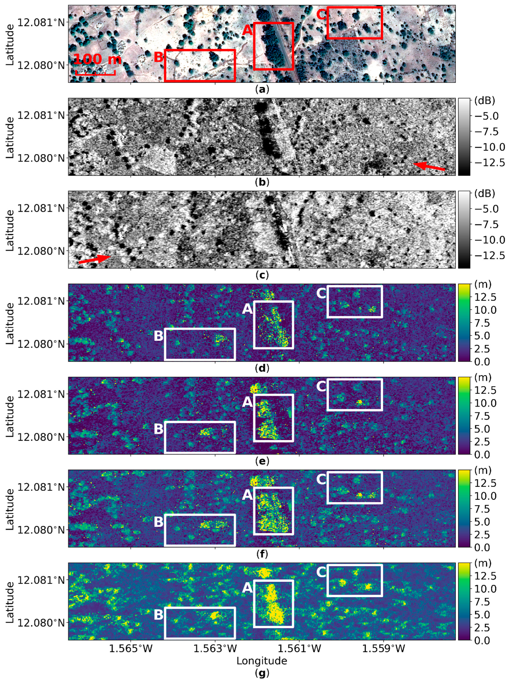
Figure 6 shows seven different images for the same 20-hectare area in Saponé. The area features a typical parkland environment, with trees of various heights and crown diameters scattered among agricultural fields (Figure 6a). Backscatter intensity images for the descending and ascending orbit directions illustrate effects of the side-looking geometry of SAR (Figure 6b,c). Shadows occur in areas obscured by the trees, while the parts of tree crowns facing the radar are brighter than the rest of the image, indicating enhanced vegetation scattering. These effects are especially prominent for the row of large trees visible in the central part of the studied area (area A in Figure 6). Varying degrees of distortion and shadowing between the ascending and descending data is due to the different incidence angles for the two orbit directions (32 degrees for descending, 25 degrees for ascending). Additionally, the oblique side-looking geometry causes a tree height-dependent ground range offset. This becomes evident when images of from descending and ascending directions are compared (Figure 6d,e): for large, tall trees, the difference between ascending and descending is larger than for smaller trees. Therefore, the combination of ascending and descending phase height images using a constant (space-invariant) offset produces an image that is blurred for some of the trees. This effect is clearly visible for areas B and C, where some trees are well focussed while others are blurred in Figure 6f, indicating different range offsets. The model-based approach proposed in Section 2.2 provides an image of , which is better focussed across different tree heights (Figure 6g). Again, this becomes obvious for areas B and C, where all trees are better focussed than in Figure 6f. Moreover, for the image of in Figure 6g, the outlines of the tree canopies are better matched with the reference satellite photo in Figure 6a, compared with the image shown in Figure 6f.
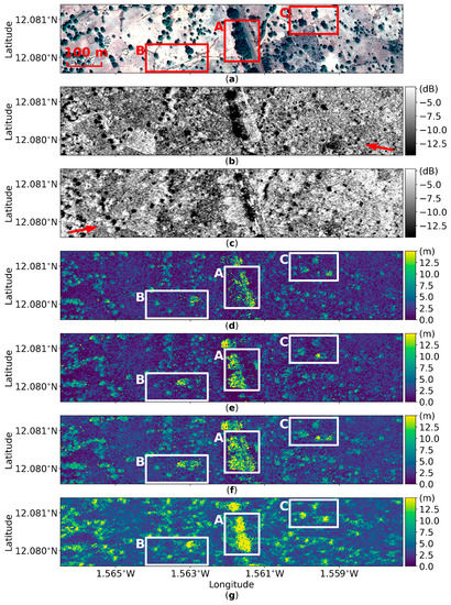
Figure 6.
Sample mapping results for a 1000 m × 200 m area in Saponé. The seven panels show: (a) orthorectified satellite image from Pléiades, backscatter coefficient () averaged across all images for the (b) descending and (c) ascending orbit directions, with red arrows indicating look directions; images of for the (d) descending and (e) ascending orbit directions; (f) image of combined from ascending and descending data; and (g) image of combined from ascending and descending data. Solid lines outline the three areas A, B, and C discussed in Section 4.1.
4.2. Tree Positioning Accuracy
Table 4 evaluates tree positioning accuracy when using maps of and . The offset between tree positions from TDM and in situ data is quantified in terms of its mean value and standard deviation in the east and north directions. Three tree height groups are used: short (up to 8 m), medium (8–16 m), and tall (above 16 m). For these three groups, the respective tree counts are: 418, 436, and 61. The results are provided separately for ascending and descending data, and for the final, combined images.

Table 4.
Tree positioning performance for phase height and mean canopy elevation images, individually for ascending and descending data and for the final, combined images. The results are provided separately for three tree height groups: short (below 8 m), medium (8–16 m), and tall (above 16 m), as well as for all trees. The biases (mean offsets) between measured and reference tree positions in the east and north directions are denoted with and , respectively, while the corresponding standard deviations are and . The highlighted values are discussed in Section 4.2.
The tree height-dependent range offset primarily manifests itself as a bias (mean offset) in the eastern direction observed in phase height images. For tall trees, the treetops are shifted on average 6.0 m in the eastern direction for the ascending orbit and −3.9 m for the descending orbit. The bias is lower for shorter trees because the co-registration routine uses spatial cross-correlation, which matches the two images using the more abundant short trees. By combining the ascending and descending data, the average bias is decreased, but the uncertainty in location is large, with the standard deviation for the east direction being 7.3 m. The corresponding values for the mean canopy elevation images are better: the tall trees are shifted in the east direction by about −0.6 m for the ascending orbit and 2.8 m for the descending orbit, and the standard deviation for height positioning in the east direction is 3.5 m. In the north direction, the bias and standard error are typically much lower and similar for both phase height and mean canopy elevation.
4.3. Tree Height Estimation
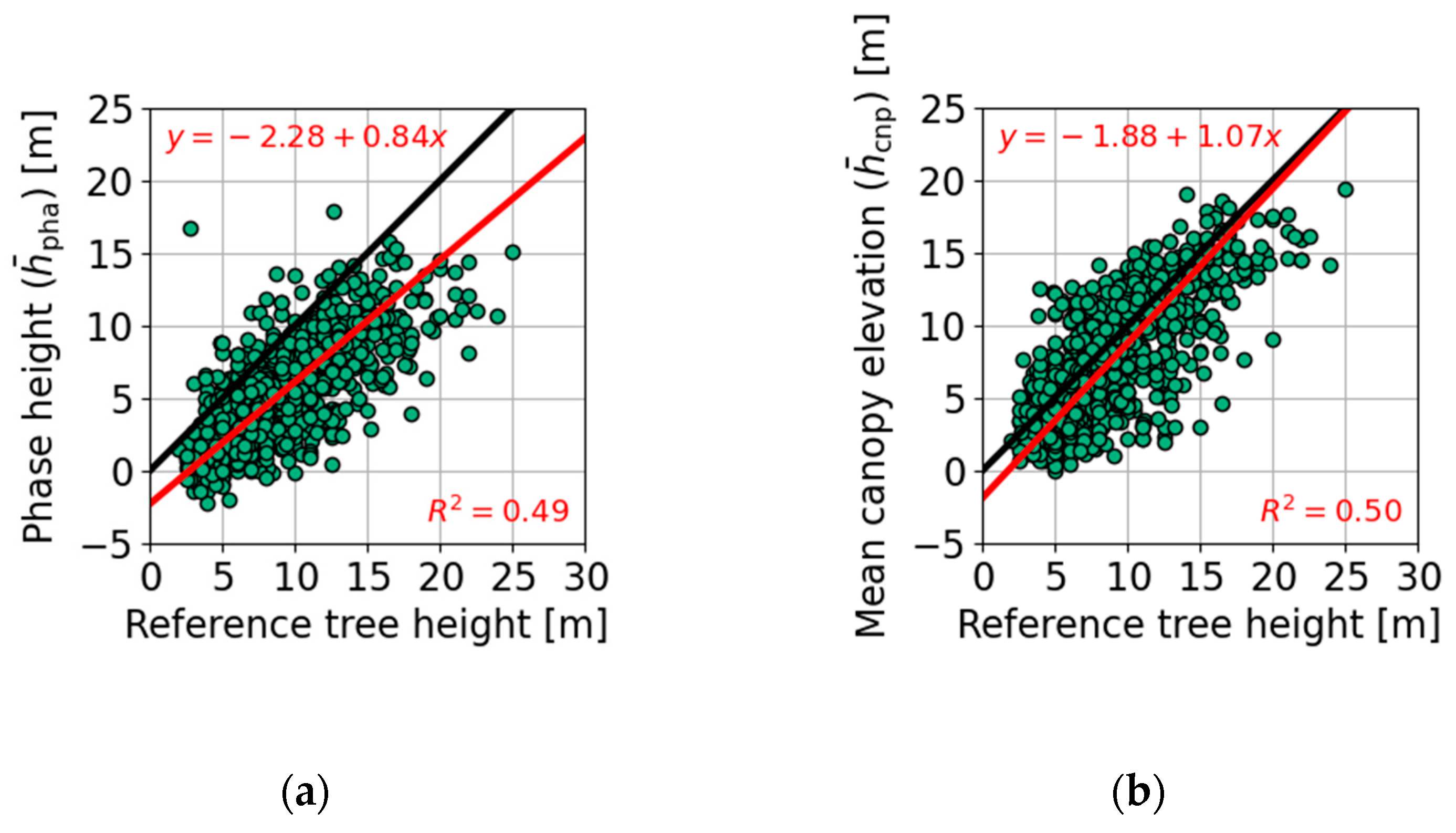
Figure 7 shows scatterplots comparing and to for all 915 trees from 15 species/genera used in this study. Bias is indicated with a red line obtained by fitting a linear function to the data using orthogonal distance regression. The corresponding bias equation is also given, together with the coefficient of determination () for the regression. The respective estimation statistics are given in Table 5.
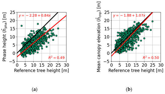
Figure 7.
Comparison of the estimated (a) phase height () and (b) mean canopy elevation () with reference in situ tree height () for all 915 trees from 15 species/genera inventoried during three field campaigns in Saponé. Green dots indicate individual trees. The solid red line describes the bias in the data, and it was obtained by fitting a linear model to the data using orthogonal distance regression. The solid black line shows the zero-bias case. The corresponding estimation statistics are shown in Table 5.

Table 5.
Tree height estimation statistics for and . “Figure” refers to the figure with the corresponding scatterplot, is the number of available tree measurements, and is the number of species/genera represented in the available tree measurements. Bias and standard error metrics are given in three tree height categories: short trees (below 8 m), medium trees (8–16 m), and tall trees (above 16 m), as well as for all trees.
The results indicate that is a biased estimator of tree height, and the bias varies with tree height. On average, for shorter trees, underestimates the tree height with over 2 m, and the underestimation increases to about 5 m for taller trees, as indicated by the red line in Figure 7a. For , the bias is on average lower, and the underestimation is consistently below 2 m, as indicated by the red line in Figure 7b. Note that for some trees, the estimated phase height is negative.
The intercept values shown in Figure 7 were subsequently used for calibration of phase height and mean canopy elevation, needed for the empirical models studied in Section 4.5: was used with (11) to obtain the calibrated phase height estimate , while was used with (12) to obtain the calibrated mean canopy height estimate .
4.4. Effect of Species/Genera on Mean Canopy Elevation
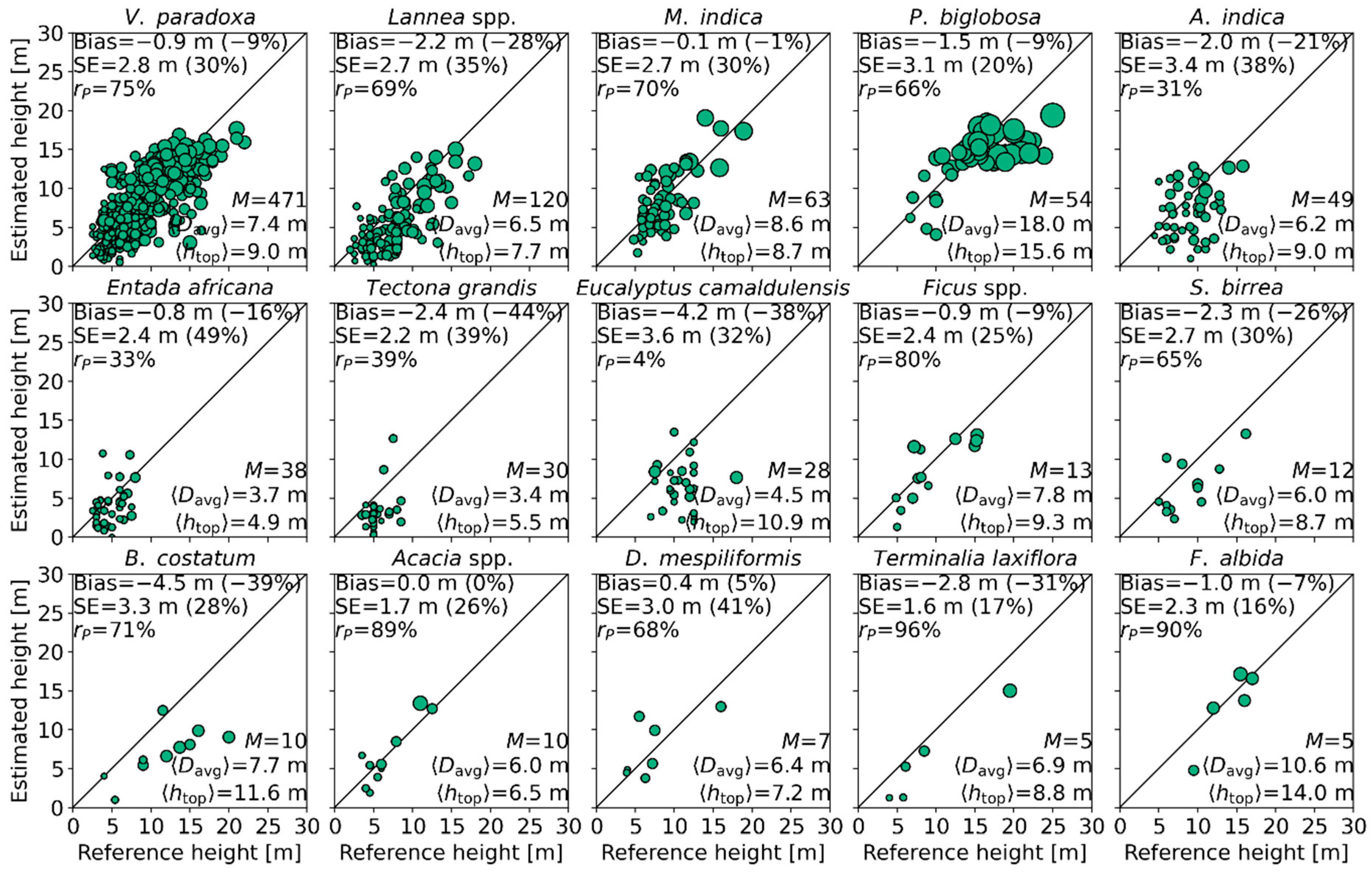
Figure 8 evaluates against , individually for each of the 15 species/genera represented in the reference data. Estimation statistics are provided, as well as the number of trees in each group and the average and . Marker sizes are proportional to .
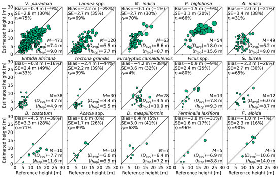
Figure 8.
Dependence of the estimated mean canopy elevation () on the in situ-measured tree height () and species/genera for the 915 trees shown in Figure 6. and are the average crown diameter and tree height for each species while is the number of trees. Marker sizes are proportional to .
For the four most abundant species/genera (V. paradoxa, Lannea spp., M. indica, and P. biglobosa), there is a clear correlation between and (with a Pearson correlation coefficient, , between 66% and 75%) and the standard error (SE) is 20–35% of the average . For the four less abundant species (Azadirachta indica A. Juss., Entada africana Guill. and Perr., Tectona grandis, and Eucalyptus camaldulensis), the correlation between and is low (4–39%), and the relative SE values are higher (32–49%). Note that these groups contain some of the smallest trees in this study: Entada africana and Tectona grandis have the lowest average and , while Eucalyptus camaldulensis and A. indica have some of the lowest average . Finally, each of the remaining seven least abundant species/genera (Ficus spp., Sclerocarya birrea (A. Rich.) Hochst., Bombax costatum Pellegr. and Vuillet., Acacia spp., Diospyros mespiliformis Hochst. ex A. DC., Terminalia laxiflora Engl. and Diels, and F. albida) shows good correlation between and (65–96%), and a relative SE of 16–41%.
The largest average bias is observed for B. costatum (−4.5 m), Eucalyptus camaldulensis (−4.2 m), and Terminalia laxiflora (−2.8 m). These species have relatively narrow tree crowns: the average is in the interval 8.8–11.6 m, while the average is in the interval 4.9–7.7 m. The smallest average bias is observed for Acacia spp. (0.0 m), M. indica (−0.1 m), and D. mespiliformis (0.4 m). In contrast to the three species with the largest bias, these species have a typically higher (6.0–8.6 m) while their average is smaller (6.5–8.7 m), indicating wider crowns. For the remaining nine species/genera, the bias is between −2.4 and −0.8 m. A relatively large bias is observed for P. biglobosa (−1.5 m), which is the tallest tree in this comparison (average of 15.6 m), with the widest crowns (average of 18.0 m).
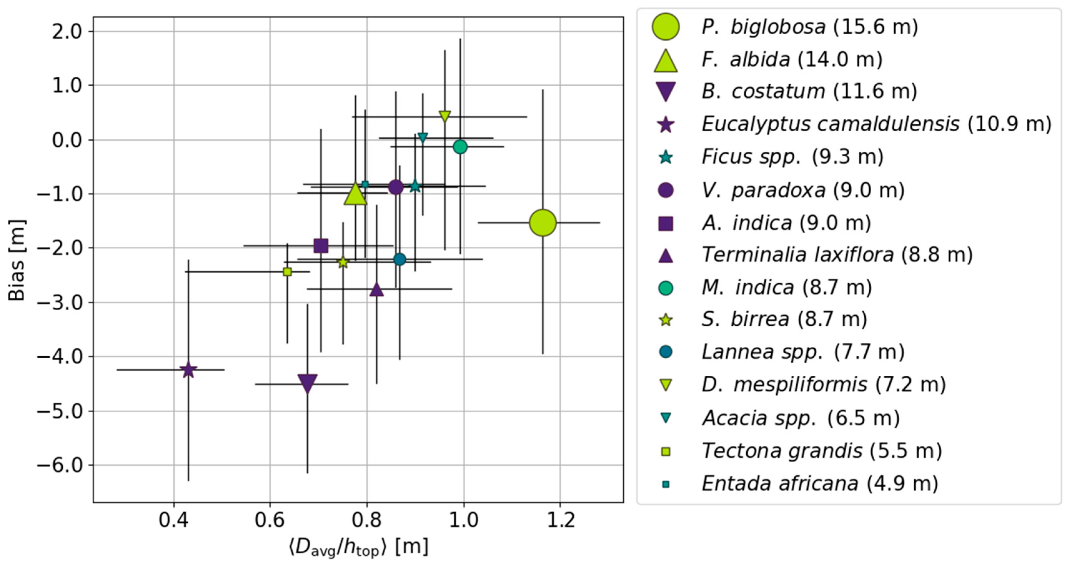
The dependence of bias on and is investigated further in Figure 9, where the bias shown in Figure 8 is plotted against the ratio, which is an indicator of crown shape. A low indicates a tall and narrow tree crown, while a high indicates a short and wide crown. Marker sizes are proportional to average and error bars are also shown, indicating the 25th and 75th percentiles of bias and .
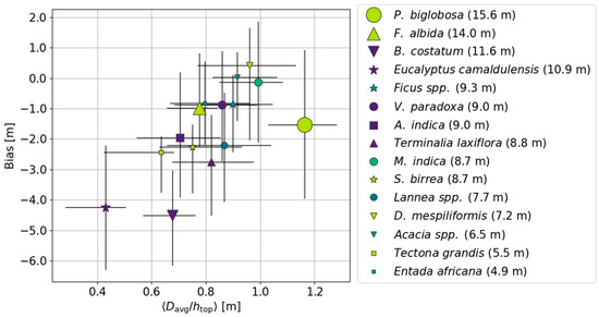
Figure 9.
Bias (from Figure 8) versus average for the 15 species/genera. Marker sizes are proportional to the average (also given in parentheses for each species/genus). The vertical and horizontal bars indicate the 25th and 75th percentile values for each quantity.
There is a correlation between bias and . A larger underestimation of observed for species/genera with low , i.e., with narrow crowns. One notable exception from the general trend is P. biglobosa, for which a negative bias is measured, compared with the positive bias that would be expected from the overall trend.
4.5. Tree Height Estimation with Empirical Models
The potential of TDM height proxies and in situ data for tree height estimation was also investigated using empirical models. Although we investigated a total of 760 models, only a small subset of the best-performing models is presented here, while the reader is referred to Supplementary Materials for a comprehensive compilation of the results for all tested models. This evaluation serves three purposes: (i) models using only TDM data assess the potential of two different techniques for TDM-based tree height measurement, (ii) models using in situ data only provide performance metrics that can be used as benchmark when assessing the remote sensing-based methods, and (iii) models combining TDM proxies with in situ data provide an interesting operational alternative for long-term monitoring of trees with some, easy-to-measure quantities accessed from the ground and height monitored from satellite. Moreover, these models also assess the potential synergies of TDM-based height estimation with future techniques capable of providing reliable estimates of, e.g., crown diameter and species.
Overall, it was found that provided better tree height estimation results than , and logarithmic models typically performed better than linear. Of the two field-measured metrics and , the latter provided better estimation results, both when used alone and in combination with the TDM-based estimates. Species-specific models provided significantly better results than species-independent models.
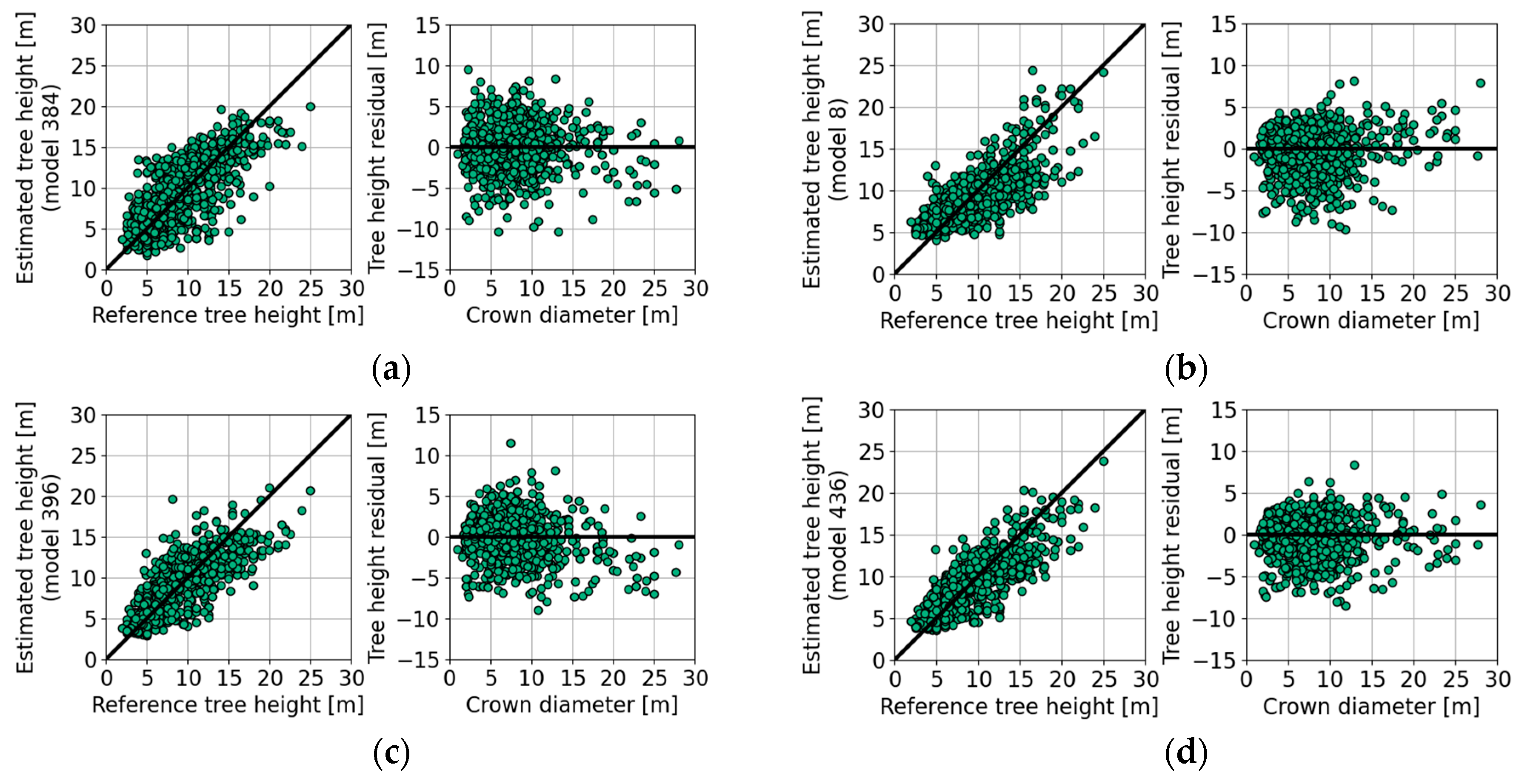
Figure 10 shows scatterplots for six selected models, while Table 6 contains mathematical expressions and performance metrics for the respective models. Each of the six models was the best-performing in terms of standard error (SE, i.e., the standard deviation of residuals) out of all tested models with that input data. In case multiple models gave the same SE (to the first decimal), the model with the fewest parameters was selected.
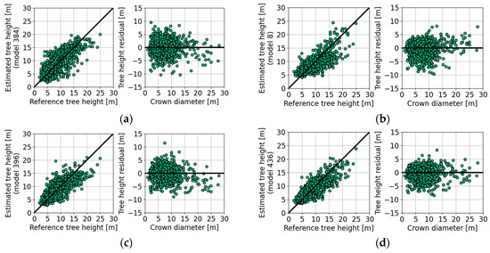

Figure 10.
Tree height estimation performance for the selected best-performing models using: (a) TDM data only, (b) only, (c) only, (d) and , (e) TDM data and species information, (f) , , and species information. Mathematical expressions and estimation statistics are shown in Table 6. For (a–d), the models were fitted to data from all 915 trees, disregarding the species/genus of the trees. For (e,f), the models were fitted individually for each species/genus with at least ten times more trees than model parameters. In each panel, the first scatterplot from the left shows the estimated tree height () on the -axis against the reference tree height () on the -axis, while the second scatterplot shows the obtained tree height residual () against average canopy diameter ().

Table 6.
Tree height estimation statistics for selected empirical models of TDM data and in situ-measurements. “Figure” refers to the figure with the corresponding scatterplot, is the total number of estimated parameters, is the number of available tree measurements, and is the number of species/genera represented in the available tree measurements. For the species-specific models, the ratio between the number of trees within each species/genus and the number of model parameters to-be-estimated was required to be at least 10, thus reducing the number of included species and the total number of trees. Bias and standard error metrics are given in three tree height categories: short trees (below 8 m), medium trees (8–16 m), and tall trees (above 16 m), as well as for all trees. This table is an excerpt from the full results that can be found in Supplementary Materials.
Using TDM data alone in an empirical model results in a correlation of 75%, an SE of 2.8 m and the error is similar for all three height groups (Figure 10a). For comparison, in situ-based measurements of average crown diameter () and diameter at breast height () give somewhat better overall results, although the performance varies more strongly with height: seems to perform better for tall trees, while is a better estimate of height for shorter trees (Figure 10b,c). Combination of and gives a correlation of 82% and an SE of 2.3 m (Figure 10d). Using species-specific models with TDM data clearly helps to mitigate some species-specific bias effects, improving the correlation to 79% and the SE to 2.6 m (Figure 10e). Finally, for comparison, the best results obtained using in situ data only with species-specific models is a correlation of 87% and an SE of 2.0 m (Figure 10f). The cases where TDM data are combined with in situ-measurements are also of interest. The results provided in Supplementary Materials indicate that together with in the best-performing empirical model gives an SE of 2.3 m and a correlation of 82% if species-independent models are used, and 2.1 m and 85%, respectively, for species-specific models.
5. Discussion
5.1. Tree Height Estimation Performance
This paper assessed the potential of spotlight-mode, interferometric TanDEM-X (TDM) data for mapping of tree height in the parklands of Burkina Faso. Two approaches were compared: one using phase height (), i.e., the elevation of an InSAR digital elevation model (DEM) above a digital terrain model (DTM); and another using mean canopy elevation () derived using a novel, model-based processing approach correcting for the side-looking geometry of SAR. The latter, more complex processing approach provided a better geometric representation of canopy height variations, better tree positioning accuracy, and better tree height estimation performance, with a standard error (SE) of 2.8 m (31% of the average tree height of 9.0 m) and a small overall bias for most trees.
To the authors’ current knowledge, no studies so far have evaluated satellite-based measurements of individual tree height in parkland areas, while only a few studies have evaluated satellite-based estimation of individual tree height or average tree height within small plots or sparsely forested areas. [31] used TDM data to estimate tree height in north-western Canada. A mean absolute error (MAE) of 0.72 m was reported for 4185 trees with an average reference height from ALS data of 2.47 m. In our study, the best model using only TDM data and all 915 trees from 15 species/genera would give a MAE of 2.3 m for an average of 9.0 m. This would translate to a relative MAE of 25%, while for [31], the corresponding value would be 29%. [57] measured individual tree height in lichen woodlands in Canadian subarctic using WorldView-3 stereo-photogrammetry. A root-mean-square error (RMSE) of 1.27 m was reported for 96 trees with heights in the interval 2–12 m. [58] used full-waveform data from the ICESat GLAS spaceborne laser scanning system to estimate average tree height within 23 1.5-hectare footprints in a savanna landscape in Kruger National Park, South Africa. The best models used in the study provided an RMSE of 2.42 m for an average tree height range of 5–22 m. [59] used repeat-pass InSAR data from Sentinel-1 and RADARSAT-2 to estimate average tree height for 11 0.1-hectare plots with average canopy height of 12.7 m. The best obtained MAE and RMSE were 1.30 m and 1.34 m, respectively.
In this study, we showed that improvement of height estimation could be obtained by combining TDM measurements with selected in situ data. In particular, the use of proved advantageous from the point of view of tree height estimation: while using alone provided estimates with SE of 2.5 m, combination of and further improved the estimation performance to an SE of 2.3 m. This observation has a practical implication: the measurement of is easy to conduct with simple tools (e.g., through circumference measurement with a measuring tape) and is not affected by canopy pruning or season, so it is expected to be more stable over time. Meanwhile, is more difficult to measure and is affected by pruning, moisture, and phenology. However, while is difficult to measure with remote sensing methods, high-resolution optical satellite images can be used to estimate [15]. For that reason, models combining TDM-based tree height metrics with are also of interest for future applications.
Furthermore, if species information is also available, then species-specific models can be derived, giving an improvement of TDM-based estimation performance and an SE of 2.6 m. Although tree species determination from satellite data is a notoriously difficult task, especially in areas where species diversity is high and the geographical extent is large [60], species do not change over time which is useful for monitoring of existing trees or plantations. The development in spatiotemporal and spectral resolution of recent satellite systems and improvements in image classification methods may pave the way for accurate tree species mapping in the near future [61].
The results obtained in this study and in [31] show that TDM has good potential for mapping and monitoring of height for individual trees, in particular in remote and/or frequently cloud-covered areas, where other measurement methods are ineffective. In this study, to get a sufficiently large dataset of tree height measurements, we used in situ data acquired up to 6 years prior to the TDM measurements. Due to the lack of suitable information on growth and pruning activities, we neglected temporal changes occurring between the in situ and TDM measurements. The unaccounted temporal changes have certainly hampered the observed estimation performance.
The analysis revealed that tree height estimation performance varies across species/genera (Figure 8). The observed underestimation was largest for tree species/genera with tall and narrow crowns, while most species with wide crown showed less bias (Figure 9). A notable exception was P. biglobosa, which showed a relatively large underestimation of tree height, despite being the tallest tree species in this comparison, with the largest tree crowns. Two potential explanations for these effects are (1) crown shape bias, caused by varying distribution of canopy objects within the topmost pixel and most prominent for trees with narrow canopies, and (2) vegetation bias from the DTM, most prominent for tall trees with wide canopies. In this paper, the observed systematic errors could be reduced with empirical models (Figure 10), but better understanding of the systematic errors is key for future large-scale use of the methods presented in this paper.
In this study, we did not observe any clear dependence of tree height estimation bias on canopy density, moisture, and phenology. However, this is most likely due to the limited temporal extent of the TDM data and the lack of reliable, quantitative information about tree canopies. Structural and moisture properties of the canopy are expected to have a significant effect on radar penetration, but dedicated follow up studies are needed before that impact can be measured.
5.2. Implementation Aspects and InSAR Data Considerations
In this study, phase height was estimated from TDM spotlight data using a low-resolution DTM derived from the same data, using a large averaging window. This approach was selected to reduce vegetation bias in the reference height model; it provided meaningful results thanks to the low canopy cover (~15%) of parklands and relatively flat topography. However, some vegetation bias could still be observed, especially for areas with tall trees with wide canopies (see Section 5.1), and the effect of topographic undulations was not studied at all. Future work should focus on improving the DTM estimation methodology used in this paper and/or synergy with topographic data provided by the current GEDI and future BIOMASS missions [39,62].
This study assessed the potential of TDM for tree height estimation, and some operational aspects were not addressed. This includes the delineation of trees in TDM data, which in this paper it was done using in situ measured position and crown diameter. Using remotely sensed estimates of tree position and crown diameter, e.g., from high resolution optical satellite data rather than in situ data is expected to generate additional uncertainties in the estimation, but it is outside the scope of this study. Furthermore, this paper disregarded geolocation and co-registration inaccuracies, shadowing of entire trees (e.g., small tree located underneath a larger tree), errors in in situ measurements, and numerical errors introduced during InSAR processing and modelling.
The proposed model-based approach to InSAR processing compensates partly for the side-looking geometry of SAR and provides an improvement in both tree positioning and tree height estimation performance, as compared with only using phase height. However, it requires complex processing and substantial InSAR data: multi-temporal, spotlight-mode acquisitions were used to ascertain high resolution and stable TLM inversion in sparsely forested areas, while the combination of ascending and descending data allowed height estimation in areas shadowed from one of the directions.
Depending on the application, phase height may be a sufficient proxy for tree height, in particular if adequate training data are available and if most trees are of similar shape, size, and structure, so that a constant ground range offset correction may be applied. However, phase height is affected by ground scattering to a larger degree than mean canopy height, which can introduce bias effects related to both ground properties and canopy cover. These, in turn, can lead to unexpected results in the data, like the negative phase height values observed in very sparsely areas in boreal forests [29]. The negative phase height values observed in Figure 7b are likely due to the combination of height calibration uncertainties and the aforementioned ground scattering effects.
Future work should address tree height estimation with the stripmap-mode TDM data used to create the global DEM [25]. These data are more abundant, and they provide a substantial advantage in terms of spatial coverage (typically 30 km × 50 km, as opposed to 10 km × 5 km for the spotlight-mode data used in this paper), albeit at the cost of azimuth resolution (typically 3.3 m, compared with 1.1 m for the spotlight-mode data).
Note that in this study, the aspect of polarimetry was ignored because only HH-polarised data were available. However, polarimetric data may provide significant additional information in parklands: the vertically oriented trunks are expected to be more exposed in these sparsely forested and relatively dry areas, thus potentially causing more polarimetric diversity at X-band than in more densely forested areas. This prospect should be addressed in follow-up studies.
6. Conclusions
This study investigated the potential of using single-polarised TanDEM-X spotlight-mode data with 1.1 m azimuth resolution for mapping tree height and position of trees of multiple species in a sparse canopy cover (~15%) parkland environment in Burkina Faso. A new, model-based InSAR processing approach was developed for this study, providing a high spatial resolution (~3 m) mean canopy elevation map for a 4200 hectare test area. These data will be used in an ongoing study focussing on the effect of trees on agriculture in parkland environments.
Tree height was estimated with a standard error of 2.8 m (or 31% of the average tree height of 9.0 m), when evaluated against in situ data from 915 trees which were from 15 species/genera and using an empirical model. Systematic variations were studied across species/genera and explained with two effects: differences in crown shape and vegetation bias from the DTM. Further improvement in tree height estimation was obtained by combining TanDEM-X data with in situ data on crown diameter, diameter at breast height, and/or species, which significantly reduced the observed biases and promised synergies with other sensors (e.g., optical data with higher spatial resolution in the future and augmented bands) and/or long-term monitoring of well-known test sites with selected in situ measurements.
To fully explore the potential of the existing TanDEM-X data, future work should focus on adapting the methodology to polarimetric and/or stripmap-mode datasets. Time series spanning different seasons should provide important insights into the effect of phenology and moisture changes in trees. Future work should also consider synergies with other remote sensing data for tree crown delineation and more accurate removal of topographic effects.
Supplementary Materials
The full results, including scatterplots and tables with performance metrics, for the 760 models studied in Section 4.5 are available online at https://www.mdpi.com/article/10.3390/rs13142747/s1.
Author Contributions
Conceptualization, M.J.S., L.E.B.E., H.R. and M.O.; methodology, M.J.S.; software, M.J.S.; validation, M.J.S. and L.M.H.U.; formal analysis, M.J.S. and L.M.H.U.; investigation, M.J.S., M.K. and L.M.H.U.; resources, M.K, J.B., H.R.B., J.S., B.T., L.E.B.E., H.R. and M.O.; data curation, M.K., H.R.B., J.S. and B.T.; writing—original draft preparation, M.J.S. and M.K.; writing—review and editing, M.J.S., M.K., J.B., H.R.B., J.S., B.T., L.E.B.E., H.R., M.O. and L.M.H.U.; visualization, M.J.S.; supervision, M.K., J.B., H.R.B., J.S., L.E.B.E., H.R., M.O. and L.M.H.U.; project administration, L.E.B.E., H.R. and M.O.; funding acquisition, L.E.B.E., H.R. and M.O. All authors have read and agreed to the published version of the manuscript.
Funding
This work was funded by the Swedish National Space Agency project: “An integrated approach to explore the unknown role of trees in dryland crop production” (dnr: 112/16).
Institutional Review Board Statement
Not applicable.
Informed Consent Statement
Not applicable.
Data Availability Statement
Not applicable.
Acknowledgments
We would like to thank Ouedarogo S. Abraham, Soro Boukary, and Ouedraogo Léonard for their assistance during field inventories; Belem Achille for introducing us to the farmers of Saponé; and the farmers of Saponé for letting us move around on their land. We would also like to thank the German Aerospace Center (DLR) for providing TanDEM-X data, support, and knowledge (project: XTI_VEGE7263). Finally, we would like to thank the anonymous reviewers for their suggestions and constructive feedback.
Conflicts of Interest
The authors declare no conflict of interest.
References
- Roupsard, O.; Audebert, A.; Ndour, A.P.; Clermont-Dauphin, C.; Agbohessou, Y.; Sanou, J.; Koala, J.; Faye, E.; Sambakhe, D.; Jourdan, C.; et al. How Far Does the Tree Affect the Crop in Agroforestry? New Spatial Analysis Methods in a Faidherbia Parkland. Agric. Ecosyst. Environ. 2020, 296, 106928. [Google Scholar] [CrossRef]
- Bargués Tobella, A.; Hasselquist, N.J.; Bazié, H.R.; Nyberg, G.; Laudon, H.; Bayala, J.; Ilstedt, U. Strategies Trees Use to Overcome Seasonal Water Limitation in an Agroforestry System in Semiarid West Africa. Ecohydrology 2017, 10, e1808. [Google Scholar] [CrossRef]
- Sanogo, K.; Binam, J.; Bayala, J.; Villamor, G.B.; Kalinganire, A.; Dodiomon, S. Farmers’ Perceptions of Climate Change Impacts on Ecosystem Services Delivery of Parklands in Southern Mali. Agrofor. Syst. 2017, 91, 345–361. [Google Scholar] [CrossRef]
- Ilstedt, U.; Tobella, A.B.; Bazié, H.R.; Bayala, J.; Verbeeten, E.; Nyberg, G.; Sanou, J.; Benegas, L.; Murdiyarso, D.; Laudon, H.; et al. Intermediate Tree Cover Can Maximize Groundwater Recharge in the Seasonally Dry Tropics. Sci. Rep. 2016, 6, 1–12. [Google Scholar] [CrossRef]
- Bayala, J.; Sanou, J.; Teklehaimanot, Z.; Kalinganire, A.; Ouédraogo, S. Parklands for Buffering Climate Risk and Sustaining Agricultural Production in the Sahel of West Africa. Curr. Opin. Environ. Sustain. 2014, 6, 28–34. [Google Scholar] [CrossRef] [Green Version]
- Karlson, M.; Ostwald, M.; Bayala, J.; Bazié, H.R.; Ouedraogo, A.S.; Soro, B.; Sanou, J.; Reese, H. The Potential of Sentinel-2 for Crop Production Estimation in a Smallholder Agroforestry Landscape, Burkina Faso. Front. Environ. Sci. 2020, 8, 85. [Google Scholar] [CrossRef]
- Bayala, J.; Sanou, J.; Teklehaimanot, Z.; Ouedraogo, S.J.; Kalinganire, A.; Coe, R.; Noordwijk, M. van Advances in Knowledge of Processes in Soil–Tree–Crop Interactions in Parkland Systems in the West African Sahel: A Review. Agric. Ecosyst. Environ. 2015, 205, 25–35. [Google Scholar] [CrossRef]
- Mechiche-Alami, A.; Abdi, A.M. Agricultural Productivity in Relation to Climate and Cropland Management in West Africa. Sci. Rep. 2020, 10, 3393. [Google Scholar] [CrossRef] [PubMed]
- Brandt, M.; Hiernaux, P.; Rasmussen, K.; Mbow, C.; Kergoat, L.; Tagesson, T.; Ibrahim, Y.Z.; Wélé, A.; Tucker, C.J.; Fensholt, R. Assessing Woody Vegetation Trends in Sahelian Drylands Using MODIS Based Seasonal Metrics. Remote Sens. Environ. 2016, 183, 215–225. [Google Scholar] [CrossRef] [Green Version]
- Papa, C.; Nzokou, P.; Mbow, C. Farmer Livelihood Strategies and Attitudes in Response to Climate Change in Agroforestry Systems in Kedougou, Senegal. Environ. Manag. 2020, 66, 218–231. [Google Scholar] [CrossRef]
- Karlson, M.; Ostwald, M. Remote Sensing of Vegetation in the Sudano-Sahelian Zone: A Literature Review from 1975 to 2014. J. Arid Environ. 2016, 124, 257–269. [Google Scholar] [CrossRef] [Green Version]
- Darkoh, M.B.K. Regional Perspectives on Agriculture and Biodiversity in the Drylands of Africa. J. Arid Environ. 2003, 54, 261–279. [Google Scholar] [CrossRef]
- Dardel, C.; Kergoat, L.; Hiernaux, P.; Mougin, E.; Grippa, M.; Tucker, C.J. Re-Greening Sahel: 30years of Remote Sensing Data and Field Observations (Mali, Niger). Remote Sens. Environ. 2014, 140, 350–364. [Google Scholar] [CrossRef]
- Heiskanen, J.; Liu, J.; Valbuena, R.; Aynekulu, E.; Packalen, P.; Pellikka, P. Remote Sensing Approach for Spatial Planning of Land Management Interventions in West African Savannas. J. Arid Environ. 2017, 140, 29–41. [Google Scholar] [CrossRef] [Green Version]
- Karlson, M.; Reese, H.; Ostwald, M. Tree Crown Mapping in Managed Woodlands (Parklands) of Semi-Arid West Africa Using WorldView-2 Imagery and Geographic Object Based Image Analysis. Sensors 2014, 14, 2643. [Google Scholar] [CrossRef]
- Lambert, M.-J.; Traoré, P.C.S.; Blaes, X.; Baret, P.; Defourny, P. Estimating Smallholder Crops Production at Village Level from Sentinel-2 Time Series in Mali’s Cotton Belt. Remote Sens. Environ. 2018, 216, 647–657. [Google Scholar] [CrossRef]
- Cho, M.A.; Mathieu, R.; Asner, G.P.; Naidoo, L.; van Aardt, J.; Ramoelo, A.; Debba, P.; Wessels, K.; Main, R.; Smit, I.P.J.; et al. Mapping Tree Species Composition in South African Savannas Using an Integrated Airborne Spectral and LiDAR System. Remote Sens. Environ. 2012, 125, 214–226. [Google Scholar] [CrossRef]
- Myeni, L.; Moeletsi, M.E.; Clulow, A.D. Present Status of Soil Moisture Estimation over the African Continent. J. Hydrol. Reg. Stud. 2019, 21, 14–24. [Google Scholar] [CrossRef]
- Forkuor, G.; Benewinde Zoungrana, J.-B.; Dimobe, K.; Ouattara, B.; Vadrevu, K.P.; Tondoh, J.E. Above-Ground Biomass Mapping in West African Dryland Forest Using Sentinel-1 and 2 Datasets—A Case Study. Remote Sens. Environ. 2020, 236, 111496. [Google Scholar] [CrossRef]
- Karlson, M. Remote Sensing of Woodland Structure and Composition in the Sudano-Sahelian Zone: Application of WorldView-2 and Landsat 8. Ph.D. Thesis, Linköping University, Linköping, Sweden, 2015. [Google Scholar]
- Ganz, S.; Käber, Y.; Adler, P. Measuring Tree Height with Remote Sensing—A Comparison of Photogrammetric and LiDAR Data with Different Field Measurements. Forests 2019, 10, 694. [Google Scholar] [CrossRef] [Green Version]
- Bamler, R.; Hartl, P. Synthetic Aperture Radar Interferometry. Inverse Probl. 1998, 14, R1–R54. [Google Scholar] [CrossRef]
- Farr, T.G.; Rosen, P.A.; Caro, E.; Crippen, R.; Duren, R.; Hensley, S.; Kobrick, M.; Paller, M.; Rodriguez, E.; Roth, L.; et al. The Shuttle Radar Topography Mission. Rev. Geophys. 2007, 45, 1–33. [Google Scholar] [CrossRef] [Green Version]
- Krieger, G.; Hajnsek, I.; Papathanassiou, K.P.; Younis, M.; Moreira, A. Interferometric Synthetic Aperture Radar (SAR) Missions Employing Formation Flying. Proc. IEEE 2010, 98, 816–843. [Google Scholar] [CrossRef] [Green Version]
- Rizzoli, P.; Martone, M.; Gonzalez, C.; Wecklich, C.; Borla Tridon, D.; Bräutigam, B.; Bachmann, M.; Schulze, D.; Fritz, T.; Huber, M.; et al. Generation and Performance Assessment of the Global TanDEM-X Digital Elevation Model. ISPRS J. Photogramm. Remote Sens. 2017, 132, 119–139. [Google Scholar] [CrossRef] [Green Version]
- Askne, J.I.H.; Fransson, J.E.S.; Santoro, M.; Soja, M.J.; Ulander, L.M.H. Model-Based Biomass Estimation of a Hemi-Boreal Forest from Multitemporal TanDEM-X Acquisitions. Remote Sens. 2013, 5, 5574–5597. [Google Scholar] [CrossRef] [Green Version]
- Solberg, S.; Astrup, R.; Breidenbach, J.; Nilsen, B.; Weydahl, D. Monitoring Spruce Volume and Biomass with InSAR Data from TanDEM-X. Remote Sens. Environ. 2013, 139, 60–67. [Google Scholar] [CrossRef]
- Kugler, F.; Schulze, D.; Hajnsek, I.; Pretzsch, H.; Papathanassiou, K.P. TanDEM-X Pol-InSAR Performance for Forest Height Estimation. IEEE Trans. Geosci. Remote Sens. 2014, 52, 6404–6422. [Google Scholar] [CrossRef]
- Soja, M.J.; Persson, H.; Ulander, L.M.H. Estimation of Forest Height and Canopy Density from a Single InSAR Correlation Coefficient. Geosci. Remote Sens. Lett. 2015, 12, 646–650. [Google Scholar] [CrossRef] [Green Version]
- Solberg, S.; May, J.; Bogren, W.; Breidenbach, J.; Torp, T.; Gizachew, B. Interferometric SAR DEMs for Forest Change in Uganda 2000–2012. Remote Sens. 2018, 10, 228. [Google Scholar] [CrossRef] [Green Version]
- Antonova, S.; Thiel, C.; Höfle, B.; Anders, K.; Helm, V.; Zwieback, S.; Marx, S.; Boike, J. Estimating Tree Height from TanDEM-X Data at the Northwestern Canadian Treeline. Remote Sens. Environ. 2019, 231, 111251. [Google Scholar] [CrossRef]
- Persson, H.; Olsson, H.; Soja, M.; Ulander, L.; Fransson, J. Experiences from Large-Scale Forest Mapping of Sweden Using TanDEM-X Data. Remote Sens. 2017, 9, 1253. [Google Scholar] [CrossRef] [Green Version]
- Lee, S.-K.; Fatoyinbo, T.E. TanDEM-X Pol-InSAR Inversion for Mangrove Canopy Height Estimation. IEEE J. Sel. Top. Appl. Earth Obs. Remote Sens. 2015, 8, 3608–3618. [Google Scholar] [CrossRef]
- Treuhaft, R.; Gonzalves, F.; dos Santos, J.R.; Keller, M.; Palace, M.; Madsen, S.N.; Sullivan, F.; Graca, P.M.L.A. Tropical-Forest Biomass Estimation at X-Band From the Spaceborne TanDEM-X Interferometer. IEEE Geosci. Remote Sens. Lett. 2015, 12, 239–243. [Google Scholar] [CrossRef] [Green Version]
- Krieger, G.; Moreira, A.; Fiedler, H.; Hajnsek, I.; Werner, M.; Younis, M.; Zink, M. TanDEM-X: A Satellite Formation for High-Resolution SAR Interferometry. IEEE Trans. Geosci. Remote Sens. 2007, 45, 3317–3341. [Google Scholar] [CrossRef] [Green Version]
- Kellndorfer, J.; Walker, W.; Pierce, L.; Dobson, C.; Fites, J.A.; Hunsaker, C.; Vona, J.; Clutter, M. Vegetation Height Estimation from Shuttle Radar Topography Mission and National Elevation Datasets. Remote Sens. Environ. 2004, 93, 339–358. [Google Scholar] [CrossRef]
- Hirt, C.; Filmer, M.S.; Featherstone, W.E. Comparison and Validation of the Recent Freely Available ASTER-GDEM Ver1, SRTM Ver4.1 and GEODATA DEM-9S Ver3 Digital Elevation Models over Australia. Aust. J. Earth Sci. 2010, 57, 337–347. [Google Scholar] [CrossRef] [Green Version]
- Solberg, S.; Astrup, R.; Gobakken, T.; Naesset, E.; Weydahl, D.J. Estimating Spruce and Pine Biomass with Interferometric X-Band SAR. Remote Sens. Environ. 2010, 114, 2353–2360. [Google Scholar] [CrossRef]
- Dubayah, R.; Blair, J.B.; Goetz, S.; Fatoyinbo, L.; Hansen, M.; Healey, S.; Hofton, M.; Hurtt, G.; Kellner, J.; Luthcke, S.; et al. The Global Ecosystem Dynamics Investigation: High-Resolution Laser Ranging of the Earth’s Forests and Topography. Sci. Remote Sens. 2020, 1, 100002. [Google Scholar] [CrossRef]
- Curlander, J.C.; McDonough, R.N. Synthetic Aperture Radar: Systems and Signal. Processing; John Wiley & Sons Inc.: Hoboken, NJ, USA, 1992. [Google Scholar]
- Cloude, S.R.; Papathanassiou, K.P. Polarimetric SAR Interferometry. IEEE Trans. Geosci. Remote Sens. 1998, 36, 1551–1565. [Google Scholar] [CrossRef]
- Soja, M.J.; Askne, J.I.H.; Ulander, L.M.H. Estimation of Boreal Forest Properties from TanDEM-X Data Using Inversion of the Interferometric Water Cloud Model. IEEE Geosci. Remote Sens. Lett. 2017, 14, 997–1001. [Google Scholar] [CrossRef]
- Soja, M.J.; Persson, H.J.; Ulander, L.M.H. Estimation of Forest Biomass from Two-Level Model Inversion of Single-Pass InSAR Data. IEEE Trans. Geosci. Remote Sens. 2015, 53, 5083–5099. [Google Scholar] [CrossRef] [Green Version]
- Soja, M.J.; Persson, H.J.; Ulander, L.M.H. Modeling and Detection of Deforestation and Forest Growth in Multitemporal TanDEM-X Data. IEEE J. Sel. Top. Appl. Earth Obs. Remote Sens. 2018, 11, 3548–3563. [Google Scholar] [CrossRef]
- Zebker, H.A.; Villasenor, J. Decorrelation in Interferometric Radar Echoes. IEEE Trans. Geosci. Remote Sens. 1992, 30, 950–959. [Google Scholar] [CrossRef] [Green Version]
- Bazié, H.R.; Bayala, J.; Zombré, G.; Sanou, J.; Ilstedt, U. Separating Competition-Related Factors Limiting Crop Performance in an Agroforestry Parkland System in Burkina Faso. Agrofor. Syst. 2012, 84. [Google Scholar] [CrossRef]
- Bayala, J.; Teklehaimanot, Z.; Ouedraogo, S.J. Millet Production under Pruned Tree Crowns in a Parkland System in Burkina Faso. Agrofor. Syst. 2002, 54, 203–214. [Google Scholar] [CrossRef]
- Karlson, M.; Ostwald, M.; Reese, H.; Sanou, J.; Tankoano, B.; Mattsson, E. Mapping Tree Canopy Cover and Aboveground Biomass in Sudano-Sahelian Woodlands Using Landsat 8 and Random Forest. Remote Sens. 2015, 7, 10017–10041. [Google Scholar] [CrossRef] [Green Version]
- Boffa, J.M. Agroforestry Parkland in Sub-Saharan Africa FAO Conservation Guide 34; United Nations Food and Agricultural Organization: Rome, Italy, 1999. [Google Scholar]
- Weather Underground Ouagadougou, Kadiogo, Burkina Faso Weather History. Available online: https://www.wunderground.com/history/daily/bf/ouagadougou/DFFD (accessed on 31 August 2020).
- GAMMA. GAMMA Remote Sensing. Available online: http://www.gamma-rs.ch (accessed on 7 September 2020).
- Duque, S.; Balss, U.; Rossi, C.; Fritz, T.; Balzer, W. TanDEM-X Payload Ground Segment, CoSSC Generation and Interferometric Considerations; Remote Sensing Technology Institute, German Aerospace Center (DLR): Köln, Germany, 2012. [Google Scholar]
- Airbus Defence & Space. Radiometric Calibration of TerraSAR-X Data: Beta Naught and Sigma Naught Coefficient Calculation; AIRBUS: Leiden, The Netherlands, 2014. [Google Scholar]
- Kass, M.; Witkin, A.; Terzopoulos, D. Snakes: Active Contour Models. Int. J. Comput. Vis. 1988, 1, 321–331. [Google Scholar] [CrossRef]
- Elmqvist, M. Ground Surface Estimation from Airborne Laser Scanning Data Using Active Shape Models. Int. Arch. Photogramm. Remote Sens. Spat. Inf. Sci. 2002, 34, 114–118. [Google Scholar]
- Nocedal, J.; Wright, S.J. Numerical Optimization, 2nd ed.; Springer Series in Operations Research; Springer: New York, NY, USA, 2006; ISBN 978-0-387-30303-1. [Google Scholar]
- St-Onge, B.; Grandin, S. Estimating the Height and Basal Area at Individual Tree and Plot Levels in Canadian Subarctic Lichen Woodlands Using Stereo WorldView-3 Images. Remote Sens. 2019, 11, 248. [Google Scholar] [CrossRef] [Green Version]
- Khalefa, E.; Smit, I.P.J.; Nickless, A.; Archibald, S.; Comber, A.; Balzter, H. Retrieval of Savanna Vegetation Canopy Height from ICESat-GLAS Spaceborne LiDAR With Terrain Correction. IEEE Geosci. Remote Sens. Lett. 2013, 10, 1439–1443. [Google Scholar] [CrossRef] [Green Version]
- Kumar, P.; Krishna, A.P. InSAR-Based Tree Height Estimation of Hilly Forest Using Multitemporal Radarsat-1 and Sentinel-1 SAR Data. IEEE J. Sel. Top. Appl. Earth Obs. Remote Sens. 2019, 12, 5147–5152. [Google Scholar] [CrossRef]
- Fassnacht, F.E.; Latifi, H.; Stereńczak, K.; Modzelewska, A.; Lefsky, M.; Waser, L.T.; Straub, C.; Ghosh, A. Review of Studies on Tree Species Classification from Remotely Sensed Data. Remote Sens. Environ. 2016, 186, 64–87. [Google Scholar] [CrossRef]
- Karlson, M.; Ostwald, M.; Reese, H.; Bazié, H.R.; Tankoano, B. Assessing the Potential of Multi-Seasonal WorldView-2 Imagery for Mapping West African Agroforestry Tree Species. Int. J. Appl. Earth Obs. Geoinf. 2016, 50, 80–88. [Google Scholar] [CrossRef]
- Quegan, S.; Le Toan, T.; Chave, J.; Dall, J.; Exbrayat, J.-F.; Minh, D.H.T.; Lomas, M.; D’Alessandro, M.M.; Paillou, P.; Papathanassiou, K.; et al. The European Space Agency BIOMASS Mission: Measuring Forest above-Ground Biomass from Space. Remote Sens. Environ. 2019, 227, 44–60. [Google Scholar] [CrossRef] [Green Version]
Publisher’s Note: MDPI stays neutral with regard to jurisdictional claims in published maps and institutional affiliations. |
© 2021 by the authors. Licensee MDPI, Basel, Switzerland. This article is an open access article distributed under the terms and conditions of the Creative Commons Attribution (CC BY) license (https://creativecommons.org/licenses/by/4.0/).

