Evaluation of the J-OFURO3 Sea Surface Net Radiation and Inconsistency Correction

Abstract

A new satellite-based product containing daily sea surface net radiation ($R_n$) values at a spatial resolution of 0.25° from 1988 to 2013, named the Japanese Ocean Flux Data Sets with Use of Remote Sensing Observations, version 3 (J-OFURO3), was recently generated and released. In this letter, the performance of the J-OFURO3 sea-surface $R_n$ product was fully evaluated by using observations from 55 global moored buoy sites. The overall accuracy was satisfactory, with root-mean-square difference (RMSD) of 24.05 and 10.76 Wm⁻² at daily and monthly scales, respectively. However, an inconsistency issue was found in the long-term variations in the J-OFURO3 sea-surface $R_n$ values in approximately 2000; this inconsistency may be due to the replacement of the input dataset. To address this issue, a simple but effective inconsistency correction method was developed and conducted in this study. The analysis results demonstrated that the variations in the corrected J-OFURO3 sea-surface $R_n$ data were more reasonable and that its daily validation accuracy was significantly improved by decreasing the bias from 4.67 to 0.27 Wm⁻² before the year 2000. Thereby, it is suggested that the inconsistency correction method should be applied before using the J-OFURO3 sea-surface $R_n$ data. However, the data users still should be cautious about another discontinuity issues caused by the quality of the input dataset itself.

1. Introduction

Sea areas cover more than 70% of Earth’s surface, and they store large amounts of energy, significantly affecting the general atmospheric and oceanic circulations [1]; therefore, global and regional climates are changed through frequent air–sea flux exchanges. Hence, accurate estimations of the oceanic heat fluxes (e.g., net radiation flux and turbulent heat flux) are of great significance for evaluating the energy balance of the Earth system. The sea surface net all-wave radiation ($R_n$) is the difference between the total downward and upward shortwave and longwave radiation on the sea surface and describes the radiative energy balance at the air–sea interface. As an essential parameter, the sea-surface $R_n$ can directly affect the heat content of the ocean and the sea-surface temperature (SST) [2]; moreover, the sea-surface $R_n$ is also one of the most important inputs to most ocean surface physical models [3]. However, the sea-surface $R_n$ has received less attention than the turbulent flux components (i.e., latent heat flux (LHF) and sensible heat flux (SHF)), and it has been either ignored or removed from simple climatology models or parameterizations in most previous studies [4].

A new satellite-based product containing radiative fluxes on the sea surface, named the Japanese Ocean Flux Datasets with Use of Remote Sensing Observations, version 3 (J-OFURO3, hereinafter), and including data from 1988 to 2013 at a 0.25° spatial resolution, was developed and recently released by Nagoya University, Japan (https://j-ofuro.scc.u-tokai.ac.jp/en/, accessed on 1 December 2019) [5]. The J-OFURO project focused on developing datasets of surface heat, momentum, and freshwater fluxes over global ice-free sea areas. J-OFURO3 is the latest version of this project and contains significant improvements over J-OFURO [6] and J-OFURO2 [7], including accuracy improvements and a new validation scheme [5]. Various parameters in J-OFURO3 have been validated with satisfactory results, such as the sea-surface LHF and SHF [5]; hence, J-OFURO3 is popular and is widely used in various applications [8,9]. J-OFURO3 provides daily net shortwave radiation ($R_{\mathit{ns}}$) and net longwave radiation ($R_{nl}$) data, and these values can be directly combined to obtain daily sea-surface $R_n$ values. The sea-surface $R_{ns}$ and $R_{nl}$ values in J-OFURO3 are calculated by subtracting the upward shortwave radiation ($R_{su}$) and longwave radiation ($R_{lu}$) from the downward shortwave radiation ($R_{\mathit{si}}$) and longwave radiation ($R_{\mathit{li}}$), respectively. Specifically, $R_{\mathit{si}}$, $R_{\mathit{li}}$, and $R_{\mathit{su}}$ are all obtained from the International Satellite Cloud Climatology Project radiative flux D-series product (ISCCP-FD) [10] comprising the period from January 1988 to February 2000 and from the Clouds and the Earth’s Energy System Synoptic Radiative Fluxes and Clouds edition 3A (CERES-3A) product at a 1° spatial resolution [11], covering the period from March 2000 to December 2013. These products were re-gridded to a spatial resolution of 0.25° over open waters, and their near-coastal areas were further processed with the creeping sea fill (CSF) extrapolation method [12], while the $R_{\mathit{lu}}$ values were calculated according to the Plank function, in which the SST values were obtained from J-OFURO3 as the ensemble median values based on multiple global sea-surface temperature products [5] and the sea-surface emissivity was defined as 0.984 [13]. Notably, J-OFURO3 only covers ice-free global oceans, and the sea-ice mask used was obtained from the operational sea-surface temperature and sea-ice analysis (OSTIA, [5]). To date, the performance of the J-OFURO3 sea-surface $R_n$ data is still unknown.

In this paper, observations from 55 moored buoy sites were collected to evaluate the performance of the J-OFURO3 sea-surface $R_n$ data from the 1988–2013 period at both daily and monthly scales over global ice-free oceans. Then the consistency of the long-term J-OFURO3 sea-surface $R_n$ data was examined and analyzed. To address the inconsistency issue, a simple correction scheme was proposed and conducted thereafter, and finally, the performance of the corrected J-OFURO3 sea-surface $R_n$ data was fully evaluated and discussed, including the spatiotemporal analysis. The objective of this paper is to inform the data users of the comprehensive performance of the J-OFURO3 sea-surface $R_n$ data and present an effective inconsistency correction scheme for this product.

2. Data and Methods

2.1. Data Processing

Sea-surface $R_n$ is not a routine measurement on the sea surface; instead, $R_{\mathit{si}}$, $R_{\mathit{li}}$, and SST (unit: K) are often measured. Hence, the sea-surface $R_n$at each moored buoy site can be calculated as follows:

$$R_{\mathit{ns}}{=R}_{\mathit{si}}\left({1 - \alpha }_{\mathit{ocean}}\right)$$

(1)

$$R_{\mathit{nl}}{=R}_{\mathit{li}} - [{\epsilon }_{\mathit{ocean}}\sigma SS{T}^4+\left({1 - \epsilon }_{\mathit{ocean}}\right)R_{\mathit{li}}]$$

(2)

$$R_n{=R}_{\mathit{ns}}{+R}_{\mathit{nl}}$$

(3)

where ${\alpha }_{\mathit{ocean}}$ is the daily sea-surface shortwave broadband albedo,${ \epsilon }_{\mathit{ocean}}$ is the daily sea-surface broadband emissivity, and $\mathsf{\sigma }$ is the Stefan–Boltzmann constant (5.67 × 10⁻⁸ W·m⁻²·K⁻⁴). The terms ${\alpha }_{\mathit{ocean}}$ and ${\epsilon }_{\mathit{ocean}}$ were usually defined as constants in many previous studies without consideration of their variations [13,14]; therefore, the use of the ${\alpha }_{\mathit{ocean}}$ dataset (2000–2013) from Feng [15] and the ${\epsilon }_{\mathit{ocean}}$ dataset (1988–2013) from Cheng [16], both of which have 0.05° spatial resolutions at the daily scale used in this study, would be more reasonable than the use of data from other studies [17,18]. Note that the ${\alpha }_{\mathit{ocean}}$ dataset starts in 2000; thus, the multiannual average daily ${\alpha }_{\mathit{ocean}}$ values from 2000 to 2013 were used for the period before 2000 (1988 to 1999) by considering the relatively lower variations in the values of this parameter from year to year. The units for all radiative components are Wm⁻², the time format is GMT, and the downward direction is positive in this study.

The $R_{\mathit{si}}$, $R_{\mathit{li}}$, and SST measurements were collected from 55 global moored buoy sites in 5 measuring networks (Table 1) and have been commonly used in previous studies [19,20]. Figure 1 shows the distribution of these buoy sites, which were mainly located within the sea areas between 50° S and 50° N. After strict quality control and a manual inspection, only the measurements with the highest quality were kept [21]. For measurements with sampling frequencies less than one day (i.e., the Ocean Sustained Inter-Disciplinary Time-Series Environment Observation System (OS) and Upper Ocean Processes Group (UOP) data), the daily mean $R_{\mathit{si}}$, $R_{\mathit{li}}$, and SST values were calculated by averaging all hourly observations as long as no missing data appeared in one day. Afterwards, the daily $R_n$ value was obtained according to Equations (1)–(3), and then the monthly $R_n$ value was calculated only when more than 60% of the daily $R_n$ samples in the corresponding month were available. Finally, totals of 56,460 daily and 1773 monthly in situ sea-surface $R_n$ samples were obtained and used for the accuracy validation.

Table 1. Information on the five measuring projects/networks.

Network	Site No	Observation Frequency	Time Span	URL
OS	6	1 h	2000–2018	dods.ndbc.noaa.gov/oceansites/ accessed on 27 May 2021
TAO	15	Daily	2000–2016	www.pmel.noaa.gov/gtmba/pmel-theme/pacific-ocean-tao accessed on 27 May 2021
RAMA	6	Daily	2004–2016	www.pmel.noaa.gov/gtmba/pmel-theme/indian-ocean-rama accessed on 27 May 2021
PIRATA	7	Daily	2006–2016	www.pmel.noaa.gov/gtmba/pmel-theme/atlantic-ocean-pirata accessed on 27 May 2021
UOP	21	1 h	1988–2016	uop.whoi.edu/index.html accessed on 27 May 2021

OS, Ocean Sustained Inter-Disciplinary Time-Series Environment Observation System [27], accessed on 1 December 2019; TAO, the Tropical Atmosphere Ocean/Triangle [28], accessed on 1 December 2019; RAMA, Research Moored Array for African–Asian–Australian Monsoon Analysis and Prediction [29], accessed on 1 December 2019; PIRATA, Pilot Research Moored Array in the Tropical Atlantic [30], accessed on 1 December 2019; UOP, Upper Ocean Processes Group [31], accessed on 1 December 2019.

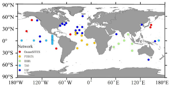
Figure 1. Distribution of 55 moored buoy sites in five measuring networks.

According to the locations of the 55 moored buoy sites, the J-OFURO3 daily sea-surface $R_n$ data, which were calculated by combining the J-OFURO3 daily $R_{\mathit{ns}}$ and $R_{\mathit{nl}}$ values directly, were extracted from 1988 to 2013 and processed into a monthly scale. The sea-surface $R_n$ data in J-OFURO3 were obtained with a spatial resolution of 0.25° from 1988 to 2013 at daily and monthly scales and then extracted according to the locations of the 55 buoy sites. Moreover, sea-surface $R_n$ data were derived from four popular reanalysis products and a ship-based product, the Japanese 55-Year Reanalysis (JRA55, 0.56° × 0.56°) from the Japanese Meteorology Administration (JMA) [22], ERA5 (0.25° × 0.25°) from the European Centre for Medium-Range Weather Forecasts (ECWMF) [23], the Modern Era Retrospective Analysis for Research and Applications, version 2 (MERRA2, 0.625° × 0.5°) [24] from NASA’s Global Modeling Assimilation Office (GMAO), the third-generation, high-resolution version of the ISCCP radiative flux profile product named ISCCP-FH (1° × 1°, 1983–2017) [25], and the ship-based product NOCS v2.0 (1° × 1°, 1973–2014) by in situ observations from voluntary observing ships contained in the International Comprehensive Ocean–Atmosphere Data Set (ICOADS) [26], extracted at daily and monthly scales from 1988 to 2013, and used for comparison in this study.

2.2. Methodology

First, the accuracy of the J-OFURO3 sea-surface $R_n$ was validated against the moored samples at both daily and monthly scales. Three commonly used statistical indices (coefficient of determination (R²), root-mean-square difference (RMSD), and bias) were applied to measure the uncertainties. Note that the in situ sea-surface $R_n$ used in this study was not the direct measurement, so it is more reasonable to use RMSD to represent the difference between J-OFURO3 and in situ sea-surface $R_n$. Then the consistency performance of the J-OFURO3 sea-surface $R_n$ dataset was assessed by examining the variations in its averaged annual mean values over global ice-free seas. After that, a correction method was proposed for addressing the inconsistency issues in the J-OFURO3 sea-surface $R_n$, as Figure 2 shows.

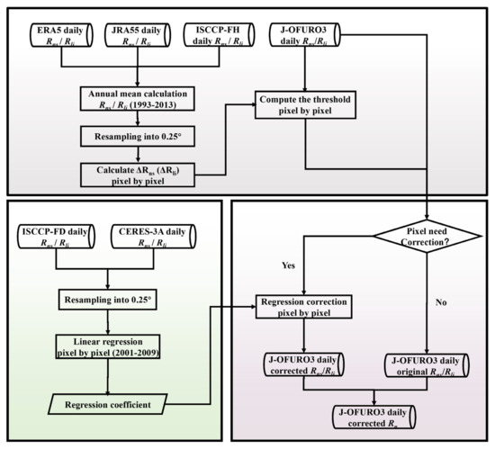
Figure 2. Flowchart of the inconsistency correction undertaken for the J-OFURO3 sea-surface $R_{\mathit{ns}}$ and $R_{\mathit{li}}$ values.

Three major steps were contained in this method. In Step 1, the thresholds were defined to determine the pixels with inconsistency issues. By considering the relatively stable performances and available time lengths, three products (ERA5, JRA5, and ISCCP-FH) were taken as the references. The differences between the average annual mean sea-surface $R_{\mathit{ns}}$ (ΔR_ns) and $R_{\mathit{li}}$ (ΔR_li) values before and after 2000 (the averages for 2000–2013, minus the averages for 1993–1999) for the three products were computed and then interpolated into a 0.25° grid, respectively; then the thresholds for each 0.25° pixel were defined as the sum of the median and the standard deviation of the ΔR_ns and ΔR_li values of the three products. In Step 2, all the J-OFURO3 pixels that needed to be corrected were determined as long as their ΔR_ns or ΔR_li values exceeded the corresponding thresholds. Then, in Step 3, because of the superiority of the performance in the CERES-3A radiation product both for land and sea surfaces, as indicated by previous studies [32,33], a set of regression models were built pixel by pixel by regressing the sea-surface $R_{\mathit{ns}}$ or R_li value from the ISCCP-FD dataset to that from the CERES-3A dataset during their overlapping period from 2001 to 2009 to correct these inconsistent pixels, and then these models were applied on the $R_{\mathit{ns}}$ and/or R_li value of these selected pixels from 1988 to 1999 by assuming that the relationships of the sea-surface $R_{\mathit{ns}}$ or R_li values between ISCCP-FD and CERES-3A remained constant. The correction model is shown in Equation (4):

$$Y=aX+b$$

(4)

where X is the daily sea-surface $R_{\mathit{ns}}$ or R_li value from the ISCCP-FD dataset from 2001 to 2009, Y is the daily sea-surface $R_{\mathit{ns}}$ or R_li value from the corresponding CERES-3A dataset from 2001 to 2009, and a and b are the regression coefficients.

Finally, the annual trends observed in the sea-surface R_n data from 1988 to 2013 were calculated by using the corrected J-OFURO3 sea-surface R_n values with a linear regression model [34], and the results were compared to those calculated from ERA5.

3. Results and Discussions

3.1. Evaluation against the In Situ Observations

Figure 3 presents the explicit spatial distribution of the J-OFURO3 multiannual mean sea-surface $R_n$ data from 1988 to 2013. The sea-surface R_n values decrease from the equatorial to the high-latitude sea areas, and nearly no data are available when the latitude is higher than 60°.

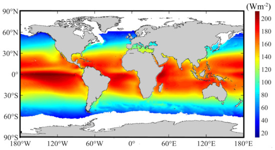
Figure 3. Multiannual mean J-OFURO3 sea-surface R_n values during the period from 1988 to 2013.

The scatter plots of the J-OFURO3 daily/monthly sea-surface $R_n$ data from 1988 to 2013 against the in situ sea-surface $R_n$ data are shown in Figure 4. The two plots show that the daily and monthly J-OFURO3 and in situ sea-surface $R_n$ values are symmetrically distributed around the 1:1 line, with overall R² values of 0.86 and 0.96, RMSD values of 24.05 and 10.76 Wm⁻², and biases of 0.16 and 0.22 Wm⁻² for the daily and monthly scales, respectively, which were similar to the results obtained by Jiang et al. [35] with RMSD of 24.712 Wm⁻².

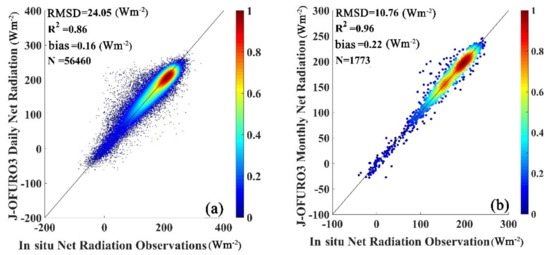
Figure 4. Scatter plots between the J-OFURO3 sea-surface $R_n$ data and the in situ measurements at (a) daily and (b) monthly scales.

Figure 5 presents the spatial distribution of the J-OFURO3 sea-surface $R_n$ uncertainties at each individual site presented with the RMSD values. The increased RMSD values from the sites in open-sea areas to those in coastal areas at both the daily and monthly scales indicate that the performance of the J-OFURO3 sea-surface $R_n$ gradually worsened; it was speculated that the worse accuracy of this dataset in coastal areas than in open-sea areas was possibly caused by pixels being extrapolated from nearby pixels, even though no satellite observations were available [12]; further quality checks should be performed in coastal areas, as pointed out by Tomita [5].

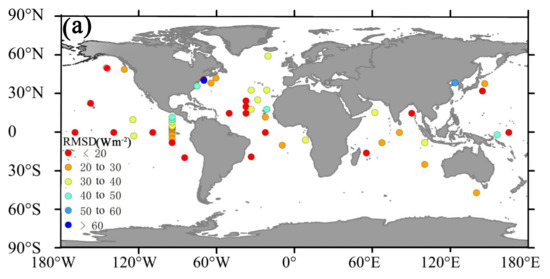
Figure 5. Spatial distribution of the RMSD of the J-OFURO3 sea-surface $R_n$ data at individual site at (a) daily and (b) monthly scales.

3.2. Inconsistency Analysis

3.2.1. Inconsistency Examination

The annual mean J-OFURO3 sea-surface $R_n$ values from 1988 to 2013 were calculated and compared with the values contained in three reanalysis products (JRA55, ERA5 and MERRA2) over the global ice-free oceans, as defined by J-OFURO3 and shown in Figure 6.

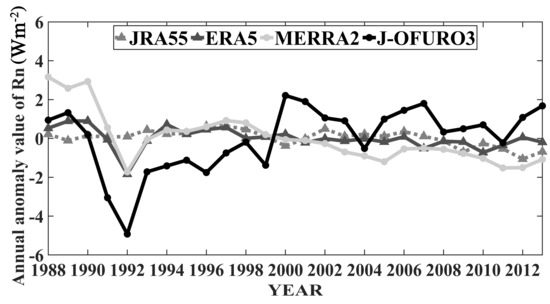
Figure 6. Interannual variations in the annual mean anomalies in the sea-surface $R_n$ values recorded from 1988 to 2013 in JRA55, ERA5, MERRA2, and J-OFURO3.

Generally, the variations in the annual mean sea-surface $R_n$ data contained in the three reanalysis products were similar to each other, with gentle but slightly decreasing trends over the past 26 years, compared to the more dissimilar trend observed in the J-OFURO3 dataset (the black line in Figure 6), especially after 2000. Moreover, two abrupt turning points were observed in the J-OFURO3, with a sudden decrease in approximately 1992 and a sharp increase during 1999/2000. The sudden drop in 1992 also appeared in the ERA5 and MERRA2 products; this drop was thought to be caused by the satellite observations taken as the inputs of the three products being influenced by the eruption of Mount Pinatubo in 1991 [36,37]. However, the other sharp increase from 1999 to 2000 with a value larger than 3 Wm⁻² only appeared in the J-OFURO3 dataset. To explore the reasonability of this sudden increase, the differences in the annual mean sea-surface $R_n$ values before 1999 and after 2000 (calculated by the means of 2000/2001 minus the means of 1998/1999) in the J-OFURO3 dataset were calculated and compared with those from the other three reference datasets of three different types, including the satellite-based product ISCCP-FD, the reanalysis product ERA5, and the ship-based product NOCS 2.0. Results shown in Figure 7 indicate that only the annual mean sea-surface R_n values of the J-OFURO3 dataset changed significantly both in magnitude and spatial distribution between the periods before 1999 and after 2000, with the values decreasing even more than 20 Wm⁻², mainly in the equatorial seas, and with increasing values over nearly all other oceans (Figure 7a); the results obtained from the other three reference datasets were more similar to each other than to the J-OFURO3 dataset (Figure 7b–d). Therefore, it was assumed that the abrupt increase observed during 1999/2000 in the J-OFURO3 sea-surface $R_n$ time series was unreasonable.

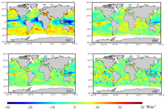
Figure 7. The differences between the average annual mean sea-surface $R_n$ values in 1998/1999 and in 2000/2001 for the (a) J-OFURO3, (b) ISCCP-FD, (c) ERA5, and (d) NOCS 2.0 datasets.

To determine the reason for this discrepancy, the consistency of each radiative component in the J-OFURO3 dataset was further examined. As mentioned above, the major radiative components ($R_{\mathit{ns}}$ and $R_{\mathit{li}}$) in the J-OFURO3 dataset were interpolated from the ISCCP-FD (before 2000) and CERES-3A datasets; hence, the average annual mean sea-surface $R_{\mathit{ns}}$ and $R_{\mathit{li}}$ values over the global ice-free oceans obtained from the two data sources (ISCCP-FD from 1988–2009 and CERES-3A from 2001–2013) were examined, and then, the SST values from J-OFURO3 during 1988–2013 were also examined, as they determined the $R_{\mathit{lu}}$ values. All results are shown in Figure 7. Obvious discrepancies were seen between ISCCP-FD and CERES-3A during their overlapping period (2000–2009) in both the sea-surface $R_{\mathit{ns}}$ (Figure 8a) and $R_{\mathit{li}}$ (Figure 8b) values, especially for $R_{\mathit{li}}$, while the relatively stable variations observed in the SST data (Figure 8c) indicated that the sharp increase in the J-OFURO3 sea-surface $R_n$ values during 1999/2000 was most likely caused by the changes in the input data sources of $R_{\mathit{ns}}$ and $R_{\mathit{li}}$ in approximately 2000.

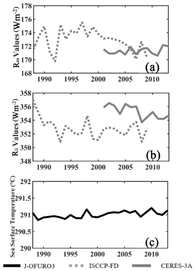
Figure 8. Interannual variations in the annual mean sea-surface (a) $R_{\mathit{ns}}$, (b) $R_{\mathit{li}}$, and (c) $\mathrm{SST}$values from 1988 to 2013 in the J-OFURO3, ISCCP-FD, and CERES-3A datasets over the global ice-free oceans.

3.2.2. Inconsistency Correction

As described in Section 2.2, the pixels with the inconsistency observed in the J-OFURO3 sea-surface $R_n$ time series in approximately 2000 were determined and then were addressed by correcting their $R_{\mathit{ns}}$ and $R_{\mathit{li}}$ values from the ISCCP-FD product before 2000 (1988–1999) to those from the CERES-3A product according to Equation (4). Figure 9 presents all pixels that needed to be corrected in J-OFURO3.

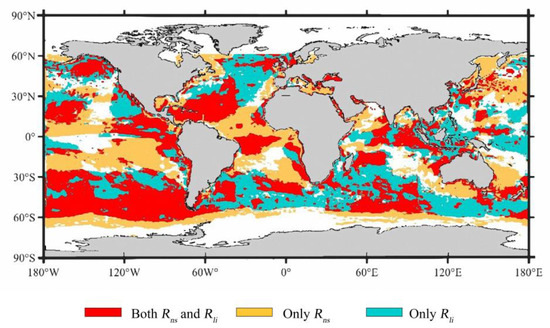
Figure 9. The determined pixels in the J-OFURO3 that needed to be corrected.

Figure 10a,b shows the interannual variations in the annual mean sea-surface $R_{\mathit{ns}}$ or R_li over the global ice-free oceans before and after the inconsistency correction. Compared to the original values, the values of the corrected sea-surface $R_{\mathit{ns}}$ and R_li and, thereby, the corrected $R_n$ values before 2000 (the black line in Figure 10) were more consistent with the values after 2000 but without much change in their variation trends; specifically, the sharp increase in approximately 2000 caused by the changes in the input datasets was eliminated in the corrected time series. After correction and comparison with the original dataset, it was found that the inconsistency issues in the J-OFURO3 sea-surface R_n were caused by different radiative component at different regions (Figure 11). Overall speaking, the inconsistency in R_n over the seas within the tropical region (20° N–20° S) was mainly caused by the inconsistent R_ns (Figure 11a); while the inconsistency in R_li lead to the inconsistent R_n over the seas for other regions (Figure 11b,c). Moreover, it shows that the corrected results before 2000 for all regions consistent with the sea-surface R_n values after 2000 very well with little changes in their variations.

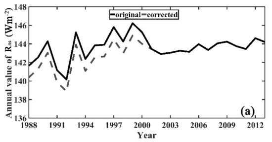
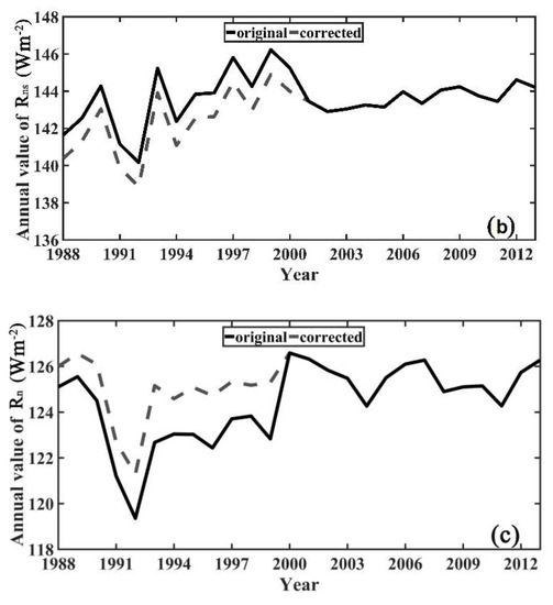
Figure 10. Interannual variations in the annual mean sea-surface (a) $R_{\mathit{ns}}$, (b) $R_{\mathit{li}}$, and (c) $R_n$ from 1988 to 2013, from the original and corrected J-OFURO3 over global ice-free oceans.

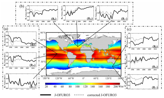
Figure 11. Interannual variations in the average annual mean sea-surface $R_n$, $R_{\mathit{ns}}$, and $R_{li}$ for three regions: (a) 20° S–20° N, (b) north of 20° N, and (c) south of 20° S from 1988 to 2013 for J-OFURO3 and corrected J-OFURO3, respectively.

The direct validation results in Figure 12 indicated that the uncertainties in the J-OFURO3 sea-surface R_n during 1988–2000 decreased significantly by reducing RMSD from 39.03 to 38.59 Wm⁻² and bias from 4.67 to 0.27 Wm⁻² respectively after correction. Taking one moored buoy site UOP-SUB-SE (18.0° N, 22.0° W) as an example, Figure 13 shows that the variations in the monthly sea-surface $R_n$ time series from the corrected J-OFURO3 in 1992 were closer to the in situ $R_n$ than the original J-OFURO3. Therefore, the inconsistency correction method was so effective that the corrected J-OFURO3 sea-surface R_n values performed more reasonably.

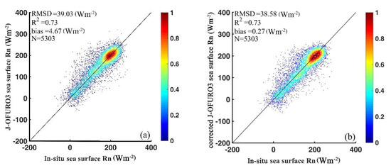
Figure 12. Scatter plots between the J-OFURO3 daily sea-surface $R_n$ and the in situ $R_n$, from 1988 to 2000, before (a) and after (b) inconsistency correction.

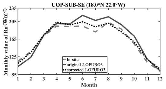
Figure 13. Times series variations in the monthly sea-surface $R_n$ in 1992 from the original corrected J-OFURO3 data and the in situ $R_n$ at the UOP-SUB-SE moored buoy site (18° N, 22° W).

However, note that the correction method proposed in this study only addressing the discontinuity issues occurring around 2000 resulted from the inputs replacement, while the other inconsistency appearing at mid–high latitude seas in approximately 2007 (Figure 11) caused by CERES-3A [38] was not addressed in this study.

3.3. Spatiotemporal Trend Analysis Based on the Corrected J-OFURO3 Sea-Surface $R_n$ Values

The spatiotemporal variations in the annual mean sea-surface $R_n$ over the tropical seas (20° N–20° S) from 1988 to 2013 were analyzed based on the corrected J-OFURO3, using the linear regression model. For comparison, the spatiotemporal analysis was also conducted on the sea-surface $R_n$ from the original J-OFURO3 and ERA5, and all results are given in Figure 14.

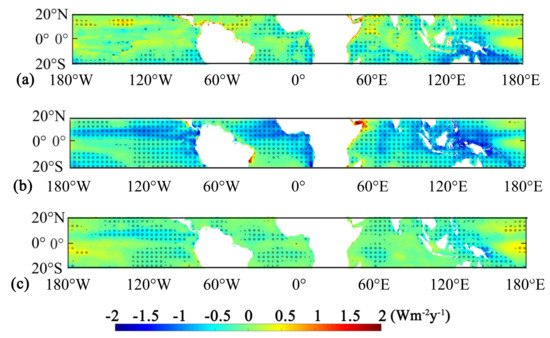
Figure 14. Spatiotemporal variations in the annual mean sea-surface $R_n$ during 1988 to 2013 by linear regression model for (a) the corrected J-OFURO3, (b) the original J-OFURO3, and (c) the ERA5. The pixels marked with a dot indicate their statistical significance, with the p-values <= 0.1.4.

Comparing with the other two datasets, the results from the corrected J-OFURO3 dataset (Figure 14a) were more consistent with the results from the ERA5 dataset (Figure 14c), which was similar to previous studies [39,40], but it had a large discrepancy with the results from the original J-OFURO3 dataset (Figure 14b), especially in the regions with increasing trends shown in Figure 14a,c. Therefore, this result again emphasized the importance and necessity of correcting the inconsistency in the original J-OFURO3 sea-surface $R_n$ time series. Specifically, based on the results obtained from the corrected J-OFURO3, the sea-surface $R_n$ increased at a mean rate of 0.257 Wm⁻² over most regions of the Western and Central Tropical Pacific, which was consistent with the studies of Liu [39] and Cook [40]. According to Cook [40], the increased sea-surface $R_n$ in this region was possibly caused by the increased $R_{\mathit{ns}}$, which were resulted from the decreased cloud amounts and the enhanced aerosol distributions or reduced water vapor droplet size. It was also seen that the sea-surface $R_n$ over the Eastern Tropical Pacific mostly decreased at a mean rate of 0.316 Wm⁻² per year, which was possibly caused by the decreased top-of-atmosphere (TOA) $R_n$ within the same region as discussed by Allan [41]. The decreased sea-surface $R_n$ would enhance the sea-surface cooling and then enhance TOA albedo, therefore further enhancing the reflected shortwave radiation and reducing the net downward energy flux radiation [42], which could explain the recent slowing rate of global surface temperature rise in this region [43,44]. Moreover, another area worth noting is the Northern Indian Ocean, where the mean trend in the J-OFURO3 sea-surface $R_n$ changed from decreasing at a rate of 0.395 Wm⁻² per year to increasing at a rate of 0.288 Wm⁻² per year after correction and this was similar to ERA5 and more reasonable. According to the studies by Arora [45], the sea-surface $R_n$ over the Tropical Indian Ocean has shown a rise trend in the recent decade because of the increased SST in this region caused by the anomalous cyclonic circulations on either side of equator and anomalous easterlies along the Tropical Pacific Ocean resulted from the weakened relation between the Indian Ocean and the Pacific Ocean [46]. Therefore, the corrected J-OFURO3 could not only provide correct tempo-spatial variations in the sea-surface R_n, but also more information on the regions different from the one from ERA5.

4. Conclusions

The sea-surface $R_n$ values obtained from a new satellite-based dataset, J-OFURO3, with a 0.25° spatial resolution from 1988 to 2013, were objectively assessed in this study. Observations collected from 55 global moored buoys in five measuring networks from 1988 to 2013 were applied to evaluate the performances of the daily and monthly J-OFURO3-derived sea-surfaces $R_n$ values; then the inconsistency problems in the J-OFURO3 sea-surface $R_n$ time series in approximately 2000 were deeply explored. Finally, a simple but effective correction method was developed and conducted. Based on all the results, some major conclusions were drawn.

• The uncertainties in the J-OFURO3 sea-surface $R_n$ were accepted, with overall R² values of 0.86 and 0.96, RMSD values of 24.05 and 10.76 Wm⁻², and biases of 0.16 and 0.22 Wm⁻² at daily and monthly scales, respectively.
• An abrupt increase appearing in approximately 2000 in the J-OFURO3 sea-surface $R_n$ time series was very possibly caused by the replacement of the input data sources from the ISCCP-FD dataset to the CERES-3A dataset.
• A simple correction method is proposed by regressing the radiative components ($R_{\mathit{ns}}$ and R_li) from the ISCCP-FD dataset to those from the CERES-3A dataset separately, pixel by pixel, and the uncertainties in the sea-surface $R_n$ were decreased remarkably by reducing the bias from 4.67 to 0.27 Wm⁻² after correction.
• The tempo-spatial variations in the J-OFURO3 sea-surface $R_n$ were more reasonable after correction especially over tropical seas.

In summary, the performance of the J-OFURO3 sea-surface $R_n$ time series was generally satisfactory, with a relative low uncertainty, and has significant potential for wide uses in various applications. However, the limitations in this product, for example, its limited coverage (only for ice-free seas), its poor performance in the near-coastal areas, and especially the inconsistency issues cannot be ignored. It is also suggested that the correction method proposed in this study should be conducted before this product is used. More efforts are needed to improve the quality of J-OFURO3. Moreover, reliable and long-time-series sea-surface $R_n$ data with high accuracy and spatiotemporal resolution are urgently required.

References

- Siegenthaler, U. The Role of Air-Sea Exchange in Geochemical Cycling; Springer: Dordrecht, The Netherlands, 1986. [Google Scholar]
- Loeb, N.G.; Lyman, J.M.; Johnson, G.C.; Allan, R.P.; Doelling, D.R.; Wong, T.; Soden, B.J.; Stephens, G.L. Observed changes in top-of-the-atmosphere radiation and upper-ocean heating consistent within uncertainty. Nat. Geosci. 2012, 5, 110–113. [Google Scholar] [CrossRef]
- Zhang, X.; McPhaden, M.J. Eastern Equatorial Pacific Forcing of ENSO Sea Surface Temperature Anomalies. J. Clim. 2008, 21, 6070–6079. [Google Scholar] [CrossRef]
- Pinker, R.T. Surface Radiative Fluxes. In Encyclopedia of Remote Sensing; Njoku, E.G., Ed.; Springer: New York, NY, USA, 2014; pp. 806–815. [Google Scholar]
- Tomita, H.; Hihara, T.; Kako, S.i.; Kubota, M.; Kutsuwada, K. An introduction to J-OFURO3, a third-generation Japanese ocean flux data set using remote-sensing observations. J. Oceanogr. 2018, 75, 171–194. [Google Scholar] [CrossRef]
- Kubota, M.; Iwasaka, N.; Kizu, S.; Konda, M.; Kutsuwada, K. Japanese Ocean Flux Data Sets with Use of Remote Sensing Observations (J-OFURO). J. Oceanogr. 2002, 58, 213–225. [Google Scholar] [CrossRef]
- Tomita, H.; Kubota, M.; Iwasaki, S.; Hihara, T.; Kawatsura, A. Introduction of J-OFURO version 2 surface heat flux data set and its analysis over the North Pacific. In Proceedings of the AGU Spring Meeting Abstracts, San Francisco, CA, USA, 9–14 December 2007. [Google Scholar]
- Small, R.J.; Bryan, F.O.; Bishop, S.P.; Tomas, R.A. Air–Sea Turbulent Heat Fluxes in Climate Models and Observational Analyses: What Drives Their Variability? J. Clim. 2019, 32, 2397–2421. [Google Scholar] [CrossRef]
- Masunaga, R.; Nakamura, H.; Kamahori, H.; Onogi, K.; Okajima, S. JRA-55CHS: An Atmospheric Reanalysis Produced with High-Resolution SST. Sola 2018, 14, 6–13. [Google Scholar] [CrossRef]
- Zhang, Y. Calculation of radiative fluxes from the surface to top of atmosphere based on ISCCP and other global data sets: Refinements of the radiative transfer model and the input data. J. Geophys. Res. 2004, 109. [Google Scholar] [CrossRef]
- Smith, G.L.; Priestley, K.J.; Loeb, N.G.; Wielicki, B.A.; Charlock, T.P.; Minnis, P.; Doelling, D.R.; Rutan, D.A. Clouds and Earth Radiant Energy System (CERES), a review: Past, present and future. Adv. Space Res. 2011, 48, 254–263. [Google Scholar] [CrossRef]
- Kara, A.B.; Wallcraft, A.J.; Barron, C.N.; Hurlburt, H.E.; Bourassa, M.A. Accuracy of 10 m winds from satellites and NWP products near land-sea boundaries. J. Geophys. Res. 2008, 113. [Google Scholar] [CrossRef]
- Konda, M.; Imasato, N.; Nishi, K.; Toda, T. Measurement of the sea surface emissivity. J. Oceanogr. 1994, 50, 17–30. [Google Scholar] [CrossRef]
- Payne, R.E. Albedo of the Sea Surface. J. Atmos. Sci. 1972, 29, 959–970. [Google Scholar] [CrossRef]
- Feng, Y.; Liu, Q.; Qu, Y.; Liang, S. Estimation of the Ocean Water Albedo From Remote Sensing and Meteorological Reanalysis Data. IEEE Trans. Geosci. Remote Sens. 2016, 54, 850–868. [Google Scholar] [CrossRef]
- Cheng, J.; Cheng, X.; Liang, S.; Niclòs, R.; Nie, A.; Liu, Q. A Lookup Table-Based Method for Estimating Sea Surface Hemispherical Broadband Emissivity Values (8–13.5 μm). Remote Sens. 2017, 9, 245. [Google Scholar] [CrossRef]
- Cheng, J.; Cheng, X.; Meng, X.; Zhou, G. A Monte Carlo Emissivity Model for Wind-Roughened Sea Surface. Sensors 2019, 19, 2166. [Google Scholar] [CrossRef]
- Hogikyan, A.; Cronin, M.F.; Zhang, D.; Kato, S. Uncertainty in Net Surface Heat Flux due to Differences in Commonly Used Albedo Products. J. Clim. 2020, 33, 303–315. [Google Scholar] [CrossRef]
- Venugopal, T.; Rahman, H.; Ravichandran, M.; Ramakrishna, S. Evaluation of MODIS/CERES downwelling shortwave and longwave radiation data over global tropical oceans. In Proceedings of the Spie Asia-Pacific Remote Sensing of the Atmosphere, Clouds, and Precipitation VI, New Delhi, India, 9 May 2016. [Google Scholar]
- Thandlam, V.; Rahaman, H. Evaluation of surface shortwave and longwave downwelling radiations over the global tropical oceans. SN Appl. Sci. 2019, 1, s42452–s43019. [Google Scholar] [CrossRef]
- McPhaden, M.J.; Busalacchi, A.J.; Cheney, R.; Donguy, J.-R.; Gage, K.S.; Halpern, D.; Ji, M.; Julian, P.; Meyers, G.; Mitchum, G.T.; et al. The Tropical Ocean-Global Atmosphere observing system: A decade of progress. J. Geophys. Res. Oceans 1998, 103, 14169–14240. [Google Scholar] [CrossRef]
- Harada, Y.; Kamahori, H.; Kobayashi, C.; Endo, H.; Kobayashi, S.; Ota, Y.; Onoda, H.; Onogi, K.; Miyaoka, K.; Takahashi, K. The JRA-55 Reanalysis: Representation of Atmospheric Circulation and Climate Variability. J. Meteorol. Soc. Jpn. Ser. II 2016, 94, 269–302. [Google Scholar] [CrossRef]
- Dee, D.P.; Uppala, S.M.; Simmons, A.J.; Berrisford, P.; Poli, P.; Kobayashi, S.; Andrae, U.; Balmaseda, M.A.; Balsamo, G.; Bauer, P.; et al. The ERA-Interim reanalysis: Configuration and performance of the data assimilation system. Quart. J. R. Meteorol. Soc. 2011, 137, 553–597. [Google Scholar] [CrossRef]
- Gelaro, R.; McCarty, W.; Suarez, M.J.; Todling, R.; Molod, A.; Takacs, L.; Randles, C.; Darmenov, A.; Bosilovich, M.G.; Reichle, R.; et al. The Modern-Era Retrospective Analysis for Research and Applications, Version 2 (MERRA-2). J. Clim. 2017, 30, 5419–5454. [Google Scholar] [CrossRef]
- Zhang, Y.-C.; Rossow, W.B.; Oinas, A.A.L.a.V. The New Long-term, Global, 3-hourly, high-resolution ISCCP-FH Atmospheric Radiative Transfer Flux Profile Product. In Proceedings of the Symposium to Celebrate William B. Rossow’s Science Contribution and Retirement, Columbia University, New York City, NY, USA, 6–8 June 2017. [Google Scholar]
- Berry, D.I.; Kent, E.C. A New Air–Sea Interaction Gridded Dataset from ICOADS with Uncertainty Estimates. Bull. Am. Meteorol. Soc. 2009, 90, 645–656. [Google Scholar] [CrossRef]
- Pagnani, M.; Galbraith, N.; Diggs. OceanSITES format and Ocean Observatory Output harmonisation: Past, present and future. In Proceedings of the Egu General Assembly Conference, Vienna, Austria, 12–17 April 2015; pp. 854–863. [Google Scholar]
- Bowman, K.P.; Phillips, A.B.; North, G.R. Comparison of TRMM rainfall retrievals with rain gauge data from the TAO/TRITON buoy array. Geophys. Res. Lett. 2003, 30. [Google Scholar] [CrossRef]
- McPhaden, M.J.; Meyers, G.; Ando, K.; Masumoto, Y.; Murty, V.S.N.; Ravichandran, M.; Syamsudin, F.; Vialard, J.; Yu, L.; Yu, W. RAMA: The Research Moored Array for African–Asian–Australian Monsoon Analysis and Prediction*. Bull. Am. Meteorol. Soc. 2009, 90, 459–480. [Google Scholar] [CrossRef]
- Bourlès, B.; Lumpkin, R.; McPhaden, M.J.; Hernandez, F.; Nobre, P.; Campos, E.; Yu, L.; Planton, S.; Busalacchi, A.; Moura, A.D.; et al. The Pirata Program. Bull. Am. Meteorol. Soc. 2008, 89, 1111–1126. [Google Scholar] [CrossRef]
- Steele, K.; Burdette, E.; Trampus, A. A System for the Routine Measurement of Directional Wave Spectra from Large Discus Buoys. In Proceedings of the OCEANS’78, Washington, DC, USA, 6–8 September 1978. [Google Scholar]
- Jia, A.; Liang, S.; Jiang, B.; Zhang, X.; Wang, G. Comprehensive Assessment of Global Surface Net Radiation Products and Uncertainty Analysis. J. Geophys. Res. Atmos. 2018, 123, 1970–1989. [Google Scholar] [CrossRef]
- Rutan, D.A.; Kato, S.; Doelling, D.R.; Rose, F.G.; Nguyen, L.T.; Caldwell, T.E.; Loeb, N.G. CERES Synoptic Product: Methodology and Validation of Surface Radiant Flux. J. Atmos. Ocean. Technol. 2015, 32, 1121–1143. [Google Scholar] [CrossRef]
- Eberly, L.E. Correlation and Simple Linear Regression. Radiology 2003, 227, 617–622. [Google Scholar]
- Bo, J.; Xiuxia, L.; Hongkai, C.; Shunlin, L.; Qiang, L.; Jie, C. Inter-comparison and evaluation of ten sea-surface net radiation estimates. J. Geophys. Res. Atmos. 2020. Submitted. [Google Scholar]
- Minnis, P.; Harrison, E.F.; Stowe, L.L.; Gibson, G.G.; Denn, F.M.; Doelling, D.R.; Smith, W.L., Jr. Radiative climate forcing by the mount pinatubo eruption. Science 1993, 259, 1411–1415. [Google Scholar] [CrossRef] [PubMed]
- Buchard, V.; Randles, C.A.; da Silva, A.M.; Darmenov, A.; Colarco, P.R.; Govindaraju, R.; Ferrare, R.; Hair, J.; Beyersdorf, A.J.; Ziemba, L.D.; et al. The MERRA-2 Aerosol Reanalysis, 1980 Onward. Part II: Evaluation and Case Studies. J. Clim. 2017, 30, 6851–6872. [Google Scholar] [CrossRef]
- Kato, S.; Loeb, N.G.; Rose, F.G.; Doelling, D.R.; Rutan, D.A.; Caldwell, T.E.; Yu, L.; Weller, R.A. Surface Irradiances Consistent with CERES-Derived Top-of-Atmosphere Shortwave and Longwave Irradiances. J. Clim. 2013, 26, 2719–2740. [Google Scholar] [CrossRef]
- Liu, C.; Allan, R.P.; Mayer, M.; Hyder, P.; Loeb, N.G.; Roberts, C.D.; Valdivieso, M.; Edwards, J.M.; Vidale, P.L. Evaluation of satellite and reanalysis-based global net surface energy flux and uncertainty estimates. J. Geophys. Res. Atmos. 2017, 122, 6250–6272. [Google Scholar] [CrossRef] [PubMed]
- Cook, K.H.; Vizy, E.K. Examining multidecadal trends in the surface heat balance over the tropical and subtropical oceans in atmospheric reanalyses. Int. J. Climatol. 2019, 40, 2253–2269. [Google Scholar] [CrossRef]
- Allan, R.P.; Liu, C.; Loeb, N.G.; Palmer, M.D.; Roberts, M.; Smith, D.; Vidale, P.L. Changes in global net radiative imbalance 1985-2012. Geophys. Res. Lett. 2014, 41, 5588–5597. [Google Scholar] [CrossRef] [PubMed]
- Brown, P.T.; Li, W.; Li, L.; Ming, Y. Top-of-atmosphere radiative contribution to unforced decadal global temperature variability in climate models. Geophys. Res. Lett. 2014, 41, 5175–5183. [Google Scholar] [CrossRef]
- Kosaka, Y.; Xie, S.P. Recent global-warming hiatus tied to equatorial Pacific surface cooling. Nature 2013, 501, 403–407. [Google Scholar] [CrossRef] [PubMed]
- Meehl, G.A.; Teng, H.; Arblaster, J.M. Climate model simulations of the observed early-2000s hiatus of global warming. Nat. Clim. Chang. 2014, 4, 898–902. [Google Scholar] [CrossRef]
- Arora, A.; Rao, S.A.; Chattopadhyay, R.; Goswami, T.; George, G.; Sabeerali, C.T. Role of Indian Ocean SST variability on the recent global warming hiatus. Glob. Planet. Chang. 2016, 143, 21–30. [Google Scholar] [CrossRef]
- Kinter, J.L.; Miyakoda, K.; Yang, S. Recent Change in the Connection from the Asian Monsoon to ENSO. J. Clim. 2002, 15, 1203–1215. [Google Scholar] [CrossRef]
Publisher’s Note: MDPI stays neutral with regard to jurisdictional claims in published maps and institutional affiliations. |
© 2021 by the authors. Licensee MDPI, Basel, Switzerland. This article is an open access article distributed under the terms and conditions of the Creative Commons Attribution (CC BY) license (https://creativecommons.org/licenses/by/4.0/).