Technical Note

New Gridded Product for the Total Columnar Atmospheric Water Vapor over Ocean Surface Constructed from Microwave Radiometer Satellite Data

1
Marine Physics and Remote Sensing Research Department, First Institute of Oceanography, Ministry of Natural Resources, Qingdao 266061, China
2
Oceanic Telemetry Engineering and Technology Innovation Center, Qingdao 266061, China
3
College of Physics, Qingdao University, Qingdao 266071, China
4
College of Geodesy and Geomatics, Shandong University of Science and Technology, Qingdao 266590, China
5
College of Marine and Information Space, China University of Petroleum (Huadong), Qingdao 266580, China
*
Author to whom correspondence should be addressed.
Remote Sens. 2021, 13(12), 2402; https://doi.org/10.3390/rs13122402
Submission received: 7 April 2021 / Revised: 15 June 2021 / Accepted: 16 June 2021 / Published: 19 June 2021
(This article belongs to the Special Issue Advances on Land–Ocean Heat Fluxes Using Remote Sensing)

Abstract

:
Based on the optimal interpolation (OI) algorithm, a daily fusion product of high-resolution global ocean columnar atmospheric water vapor with a resolution of 0.25° was generated in this study from multisource remote sensing observations. The product covers the period from 2003 to 2018, and the data represent a fusion of microwave radiometer observations, including those from the Special Sensor Microwave Imager Sounder (SSMIS), WindSat, Advanced Microwave Scanning Radiometer for Earth Observing System sensor (AMSR-E), Advanced Microwave Scanning Radiometer 2 (AMSR2), and HY-2A microwave radiometer (MR). The accuracy of this water vapor fusion product was validated using radiosonde water vapor observations. The comparative results show that the overall mean deviation (Bias) is smaller than 0.6 mm; the root mean square error (RMSE) and standard deviation (SD) are better than 3 mm, and the mean absolute deviation (MAD) and correlation coefficient (R) are better than 2 mm and 0.98, respectively.

Graphical Abstract

1. Introduction

Water vapor is an important indicator of Earth’s climate system and serves as the dominant greenhouse gas, having higher absorption than carbon dioxide. Moreover, it is a rich and important radiative atmospheric component that occurs for short times in the atmosphere [1]. Under pure natural control, water vapor variability exerts strong positive feedback on climate change [2,3], and it is also one of the major error sources when attempting precise positioning with the Global Navigation Satellite System (GNSS) [4]. Columnar atmospheric water vapor denotes the total gaseous water contained in a vertical column of the atmosphere, which corresponds to the absolute amount of water dissolved in the air.
Columnar water vapor observation methods mainly include radiosondes [5], ground-based GPS receivers [6], satellite remote sensing including optical remote sensing [7] and satellite microwave radiometers [8], differential absorption lidar (DIAL) [9], and Raman lidar [10]. The spatial and temporal coverage of ground-based measurement data is limited, and optical remote sensing is affected by rigid weather conditions. The scanning range of the spaceborne microwave radiometer reaches approximately 1000 km, which could cover more than 90% of the global ocean area every day and provide important data to monitor the changes in columnar atmospheric water vapor over the global ocean surface. The acquisition of near real-time, large-scale atmospheric water vapor information is mainly dependent on the measurements from continued satellite microwave radiometers. At present, on-orbit microwave radiometers that can be used to retrieve atmospheric water vapor mainly include NASA Aqua’s Advanced Microwave Scanning Radiometer for Earth Observing System sensor (AMSR-E), the Tropical Rainfall Measuring Mission Microwave Imager (TMI), the Special Sensor Microwave Imager (SSM/I) aboard the Defense Meteorological Satellite Program (DMSP) satellites, Coriolis WindSat, etc. However, due to the influence of clouds and rain, the effectiveness of data coverage for these microwave radiometers varies in space and time. An effective method of obtaining a daily available global mean product of atmospheric water vapor is to merge satellite observations from multiple sources.
Currently, a popular water vapor fusion technique is to make use of products derived from meteorological satellite remote sensing images. Huber proposed a method of sparse representation in 1985 [11], and Lei Wang et al. [12] proposed a fusion method with coupled sparse representation for infrared and water vapor cloud maps, which outperformed traditional pixel averaging and wavelet transform methods. Kai Liu [13] applied multiresolution analysis and multiscale geometric analysis fusion methods to conduct fusion experiments based on infrared and water vapor maps. In their experiment, the fused images showed visually good results and highlighted water vapor edge information. To our knowledge, limited types of research have attempted to generate remote sensing fusion products of global ocean columnar atmospheric water vapor from multisource satellite water vapor product data. The remote sensing system (RSS) has merged microwave radiometer data from the SSM/I [14], Special Sensor Microwave Imager Sounder (SSMIS), GMI, TMI [15], WindSat, Advanced Microwave Scanning Radiometer 2 (AMSR2), and AMSR-E [8] to a monthly average global ocean columnar atmospheric water vapor product with a spatial resolution of 1°×1°. In an attempt to better describe the dynamic changes in water vapor, a water vapor product with a higher spatial and temporal resolution is of great necessity. Therefore, this study focuses on producing a gridded, blended columnar atmospheric water vapor product with high spatial and temporal resolution based on multisource microwave data.
A variety of fusion algorithms have been proposed, including the successive correction method [16], blended analysis method [17], objective analysis method [18], Kalman filter method [16], and optimal interpolation (OI) method [19,20,21]. The characteristics of these methods were introduced in a previous article by the authors [22]. Compared with the other methods, the OI method is characterized by a higher efficiency with low computation and can be explored to obtain the global fusion product with better precision.
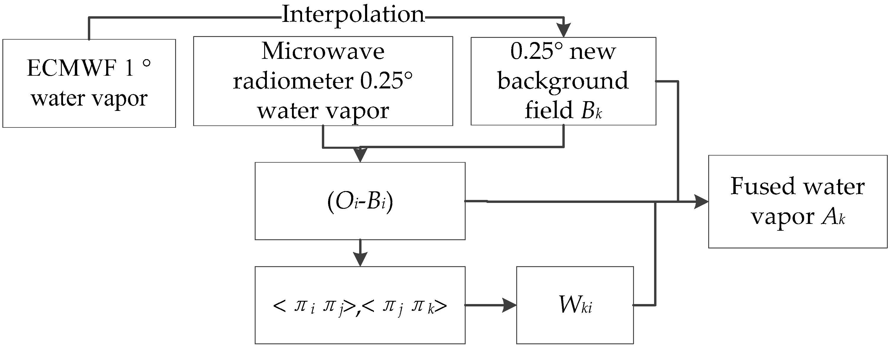
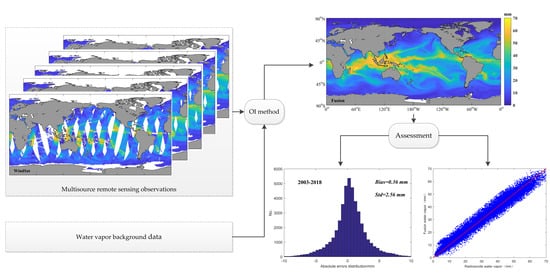
This study used a columnar atmospheric water vapor product from five satellite-borne microwave instrument sets: the AMSR-E, AMSR2 [23], WindSat, SSMIS, and HY-2A microwave radiometer (MR) [24]. Compared with the RSS dataset, the new daily available columnar atmospheric water vapor product has a better spatial resolution of 0.25°. Using the OI method, a new 0.25°/daily high spatial and temporal resolution fusion water vapor product from 2003 to 2018 was generated. The accuracy of the established atmospheric water vapor fusion products was verified using radiosonde observation data. The technical process of this study is shown in Figure 1.

2. Materials and Methods

2.1. Materials

2.1.1. Satellite Remote Sensing Data

The global ocean columnar atmospheric water vapor fusion product was obtained by using multiple satellite observations from ASMR-E, ASMR2, WindSat, and SSMIS. Additionally, water vapor data obtained from the microwave radiometer onboard HY-2A, China’s first ocean dynamic environment satellite, were also employed in the fusion process. The general information in the water vapor dataset of the satellite borne radiometer is summarized in Table 1.
SSMIS, WindSat, AMSR-E, and AMSR2 data were provided by RSS at a spatial resolution of 0.25°, and the datasets include water vapor, wind speed, and cloud liquid water data. To control the water vapor quality, outliers beyond the range of 0–70 mm were eliminated based on the GCOM-W1 Shizuku Data Users Handbook [25]. HY-2A microwave radiometer data were provided by the National Satellite Ocean Application Service (NSOAS) for L2 level products, including various sea–air parametric products of the HY-2A microwave radiometer. Additionally, quality control was performed for HY-2A water vapor data to retain the data within the normal range (0–70 mm). Using the HY-2A MR L2 swath data product, we developed a 0.25° grid data product based on the drop-in-the-box algorithm [26]. To further ensure the accuracy of the fusion results, water vapor data for all the above microwave radiometers that have an absolute deviation greater than 10 mm (greater than 3 times the standard deviation) of the corresponding background field data were excluded.

2.1.2. Water Vapor Background

Water vapor reanalysis data from the European Centre for Medium-Range Weather Forecasts (ECMWF) were used as the background field data. ECMWF provides European Reanalysis (ERA) interim (i.e., ERA-Interim) 1°/daily water vapor four times per day (at 00:00:00, 06:00:00, 12:00:00, and 18:00:00). In this study, the four ERA data points were used to generate the daily water vapor average as the first-guess field.

2.1.3. Radiosonde Data

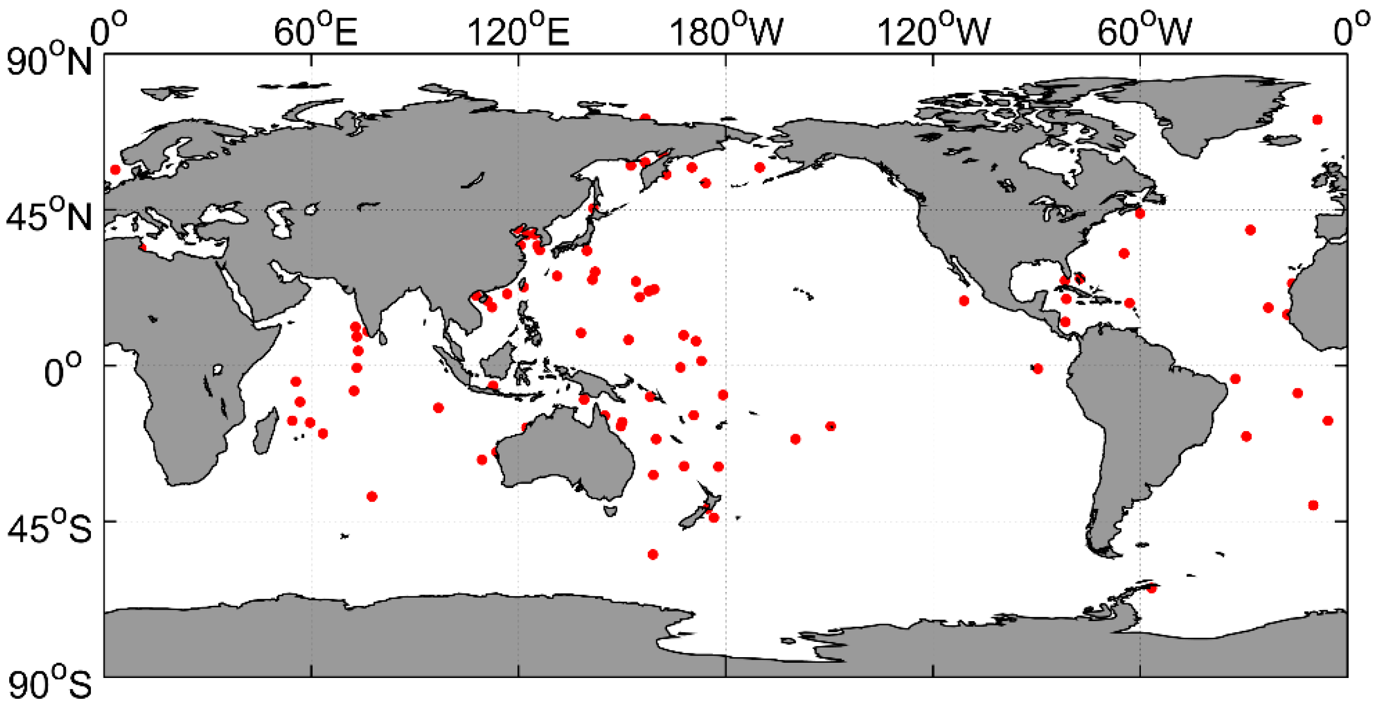
Data from more than 1000 global radiosonde stations provided by the National Centers for Environmental Information (NCEI) and from 90 stations located in the oceanic region were collected. The locations of the radiosonde stations are shown in Figure 2. All atmospheric profile data measured from 2003 to 2018 were extracted, and then the atmospheric water vapor was calculated. Because the radiosonde cannot directly measure the water vapor, the atmospheric water vapor density is calculated by using the altitude, atmospheric temperature profile, and relative humidity profile data measured by the radiosonde, and the column water vapor is obtained by the vertical integration of the water vapor density, which is used to validate the accuracy of the new water vapor product.
ρ V = 1.739 × 10 9 × R H × θ 5 × exp ( 22.64 θ ) θ = 300 / T
where ρ V is atmospheric vapor density (g/cm3), T is atmospheric temperature profile data (°C), and RH is atmospheric relative humidity profile data (%).
The validity of the calculation results was then checked; radiosonde data with the highest measurement heights less than 10,000 m were eliminated, and outliers from 0 to 70 mm were excluded. The spatial distribution of the radiosonde stations used is shown in Figure 1.

2.2. Methods

2.2.1. Water Vapor Remote Sensing Product Fusion Algorithm

The OI algorithm is used for the production of water vapor fusion products. The OI algorithm minimizes the analytical variance of the solution as long as the background, observations, and analytical fields are deemed unbiased estimates [21,22]. It is widely used in the production of data products, such as sea surface temperature [27] and wind fields [28]. According to the OI algorithm, the final value on the fused product grid point k, i.e., the water vapor content fusion value Ak, is calculated as follows:
A k = B k + i = 1 N ( O i B i ) W k i
where Bk is the background field (first guess) value at the fusion grid point k, Oi is the water vapor value measured by the microwave radiometer, Bi is the background value at the microwave radiometer observation point grid i. OiBi is the difference between the radiometer inversion value and the background field value, and Wki is the corresponding least-square weight factor, which is obtained by minimizing the variance and water vapor of the analyzed field. In the case with no radiometer observations near a grid point (distance thresholds of λ x and λ y , which are calculated below), the weight is taken as 0, and background values are adopted. N is the number of observation points near the fusion product grid k. According to the least squares principle, for the weighting factors, we have the following:
W k i i = 1 N M i j = π j π k
where M i j = π i π j + ε i 2 δ i j is the expected value of the background field correlation error, and ε i is the ratio of the data error at point i to the standard deviation of the background field, which is taken as 0.5.
δ i j = { 1 i = j 0 i j
The expected value of the background field correlation error can be expressed as follows:
π i π j = exp [ ( x i x j ) 2 λ x 2 + ( y i y j ) 2 λ y 2 ]
where x and y represent the zonal and meridional distances of the grid data, respectively; and λ x and λ y are the zonal and meridional correlation scales of water vapor, calculated as 238 and 179 km, respectively [22]. Each weighting factor of grid point k can be obtained by solving the linear equation system (3).
To obtain the (OiBi) values before data fusion, we developed a new 0.25° background field (Bk) using a 1° water vapor background. The flow of the fusion algorithm is shown in Figure 3.

2.2.2. Validation Method

The assessment of the global ocean water vapor product using radiosonde data requires the average of the radiosonde data from the same station on the same day. To do this, the proximate observation date of the radiosonde data with the water vapor fusion product was identified, and a spatial window of 0.25° for data matching was used.
The quality evaluation indicators include the mean deviation (Bias), mean absolute deviation (MAD), standard deviation (SD), root mean square error (RMSE), and correlation coefficient (R). Bias reflects the systematic deviation of the fused water vapor from the radiosonde-measured water vapor and indicates the degree of dispersion of the fused water vapor from the radiosonde-measured water vapor. MAD can avoid the positive and negative offsets of deviation and can better reflect the system deviation. SD represents the dispersion of deviation to Bias, and RMSE is used to indicate the accuracy of the fused water vapor compared to the measured water vapor of the radiosonde. The abovementioned parameters are defined in Equations (6)–(9) as follows:
B i a s = 1 N i = 1 N ( A i B i )
R M S E = 1 N i = 1 N ( A i B i ) 2
S D = i = 1 N [ ( A i B i ) ( A B ¯ ) ] 2 N
R = i = 1 N [ ( A i A ¯ ) ( B i - B ¯ ) ] i = 1 N ( A i A ¯ ) 2 i = 1 N ( B i B ¯ ) 2
where N denotes the total number of matched data between the water vapor fusion and radiosonde data, A represents the fused water vapor, and B corresponds to the radiosonde-measured water vapor.

3. Results

3.1. Remote Sensing Fusion Product

The OI algorithm is applied to merge the atmospheric water vapor results retrieved from the HY-2A MR, SSMIS, WindSat, AMSR-E, and ASMR2 microwave radiometers. As a result, a total of 16 years of global daily oceanic atmospheric water vapor remote sensing fusion product data from 2003 to 2018 were generated with a resolution of 0.25° × 0.25°. The time range began from 1 January 2003 through 31 December 2018. All products were formatted as NetCDF, which includes datasets of water vapor, grid information of latitude and longitude (grid number 720 × 1440), and ancillary information, which illustrates the data product production agency, production date, and time. The data products recorded three sets of data fields: longitude (lon), latitude (lat), and global ocean columnar atmospheric water vapor (water vapor). The longitude covered a range of 0.125°E–359.875°E, with 3 decimal places reserved; the data were available with a floating-point type. The latitude spanned a range of 89.875°S–89.875°N, with 3 decimal places reserved, and the data were stored with the floating point type. The valid range of water vapor data was 0–70,000, with an invalid value of −999 and a scale factor of 0.001, and the data type is an integer. A sample of the global ocean atmospheric water vapor fusion product on 1 January 2018 is shown in Figure 4. As shown in Figure 4, the missing areas of each single satellite data can complement each other well, and the fusion data can largely fill the gaps of each single satellite data and generate the water vapor product over the global ocean surface.
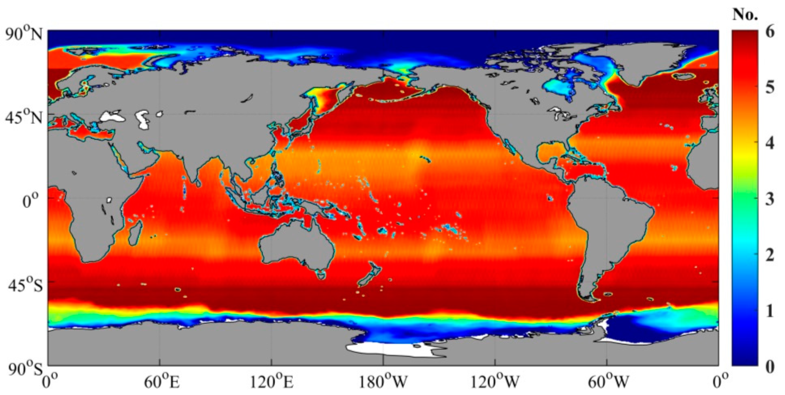
The data coverage of the microwave radiometer is defined as the proportion of the effective observation data grid to the global ocean grid. Figure 5 shows the daily coverage of these multisource spaceborne radiometer data in 2018. As shown in Figure 5, the daily coverage in 2018 fluctuated between 80% and 84%. To better describe the data coverage over the global ocean, the daily average multisource spaceborne radiometer data coverage map in 2018 is given, as shown in Figure 6. Except for the sea ice areas in the North and South Poles, at least one satellite radiometer data point is included in one grid. The data coverage over the mid-latitude ocean is better, and the coverage in the low-latitude region is slightly lower than that in the mid-latitude region due to the influence of satellite orbits. This finding also shows that the background data can be corrected by using multisource satellite observations.

3.2. Precision Validation of Fusion Products Over the Past 16 Years

The generated global oceanic atmospheric water vapor fusion data for all 16 years from 2003 to 2018 were compared with the corresponding radiosonde data with a 0.25° spatial window and a 1 day temporal window. A total of 45,198 matched data pairs were obtained, and the Bias, MAD, RMSE, and R were calculated for the water vapor product, as shown in Table 2.
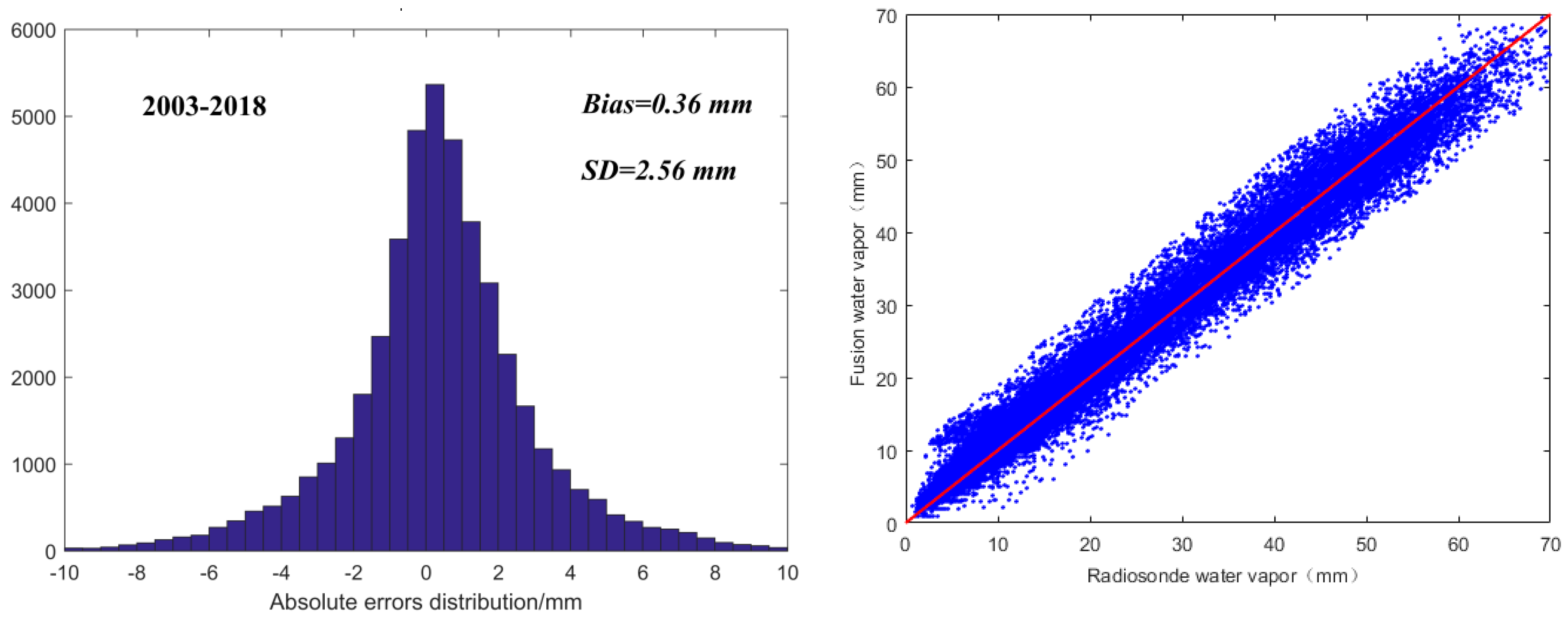
Table 2 shows that the RMSE and SD of the water vapor fusion results are better than 3 mm. Positive deviations smaller than 0.6 mm were observed for Bias and those better than 2 mm were observed for MAD, while R was stronger than 0.98. An analysis of the error distribution of remotely sensed fused water vapor and radiosonde water vapor from 2003 to 2018 was carried out to visually illustrate the comparison over the past 16 years. As shown in Figure 7, the errors presented a normal distribution, with a slight bias toward positive values. The overall estimated Bias was 0.36 mm (95% confidence interval: 0.33–0.38 mm), and the SD was 2.56 mm (95% confidence interval: 2.54–2.58 mm). A high correlation was found between the two water vapor datasets.
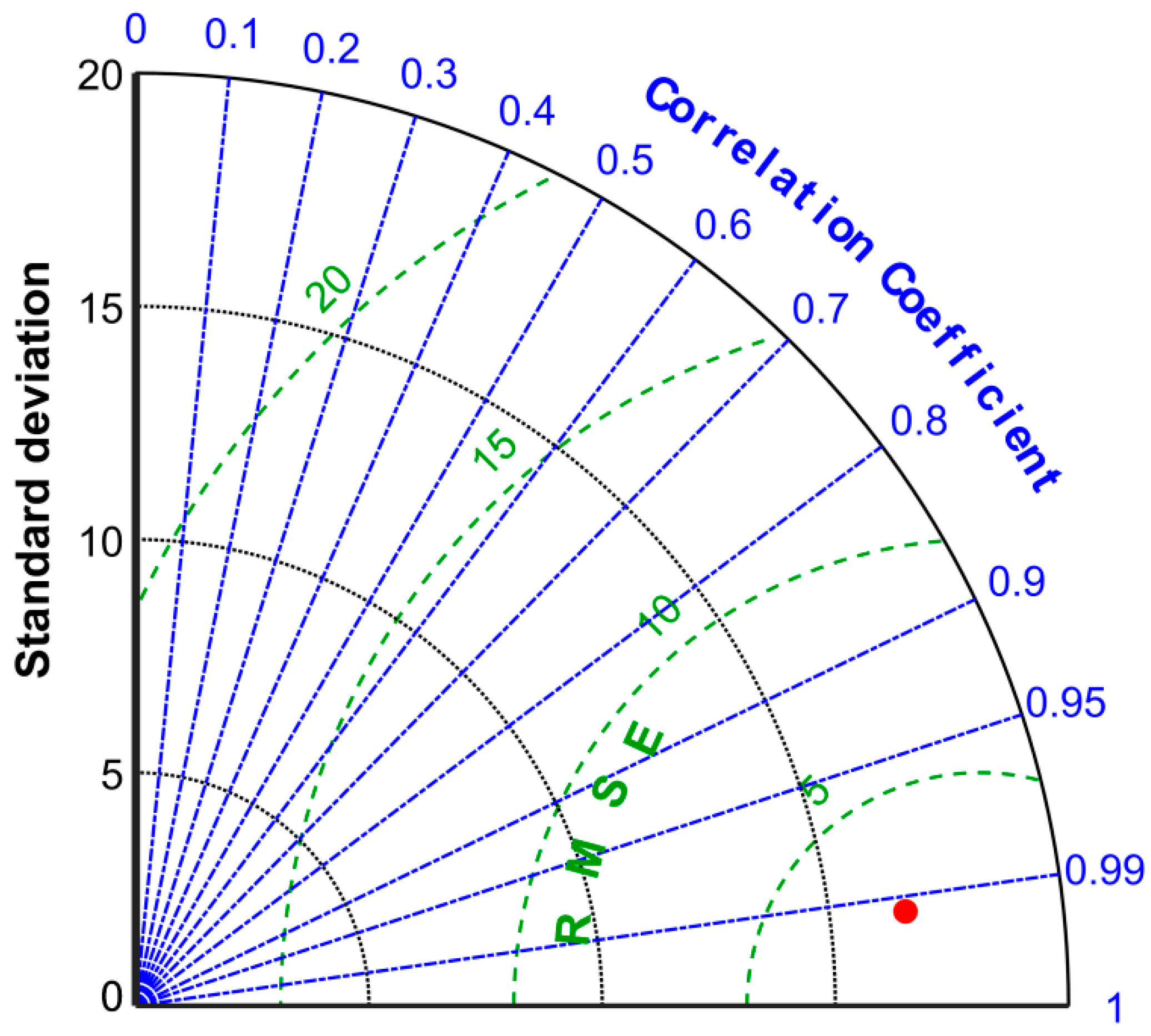
A Taylor diagram was drawn to show the robustness of the results using the fusion product and the radiosonde data in 2018, as shown in Figure 8. In the Taylor diagram, the red point represents the fusion product. The Y-axis denotes the standard deviation (SD) of the data, the radial blue line corresponds to the correlation coefficient (R), and the green dotted line represents the RMSE. Figure 8 suggests that the correlation coefficient between the fusion product and the field data was very strong, with a correlation of approximately 0.99, an RMSE of 2.36 mm, and a standard deviation close to the RMSE.
To examine the improvement of the water vapor fusion product relative to the ERA-Interim background data, the ERA-Interim background data from 2016 to 2018 were selected to verify the accuracy of the radiosonde data (Table 3). Table 2 and Table 3 show that compared with the water vapor ERA-Interim background data, the accuracy of the water vapor fusion product has been improved, which is likely due to the modification of the background data by the more accurate satellite water vapor observation data.
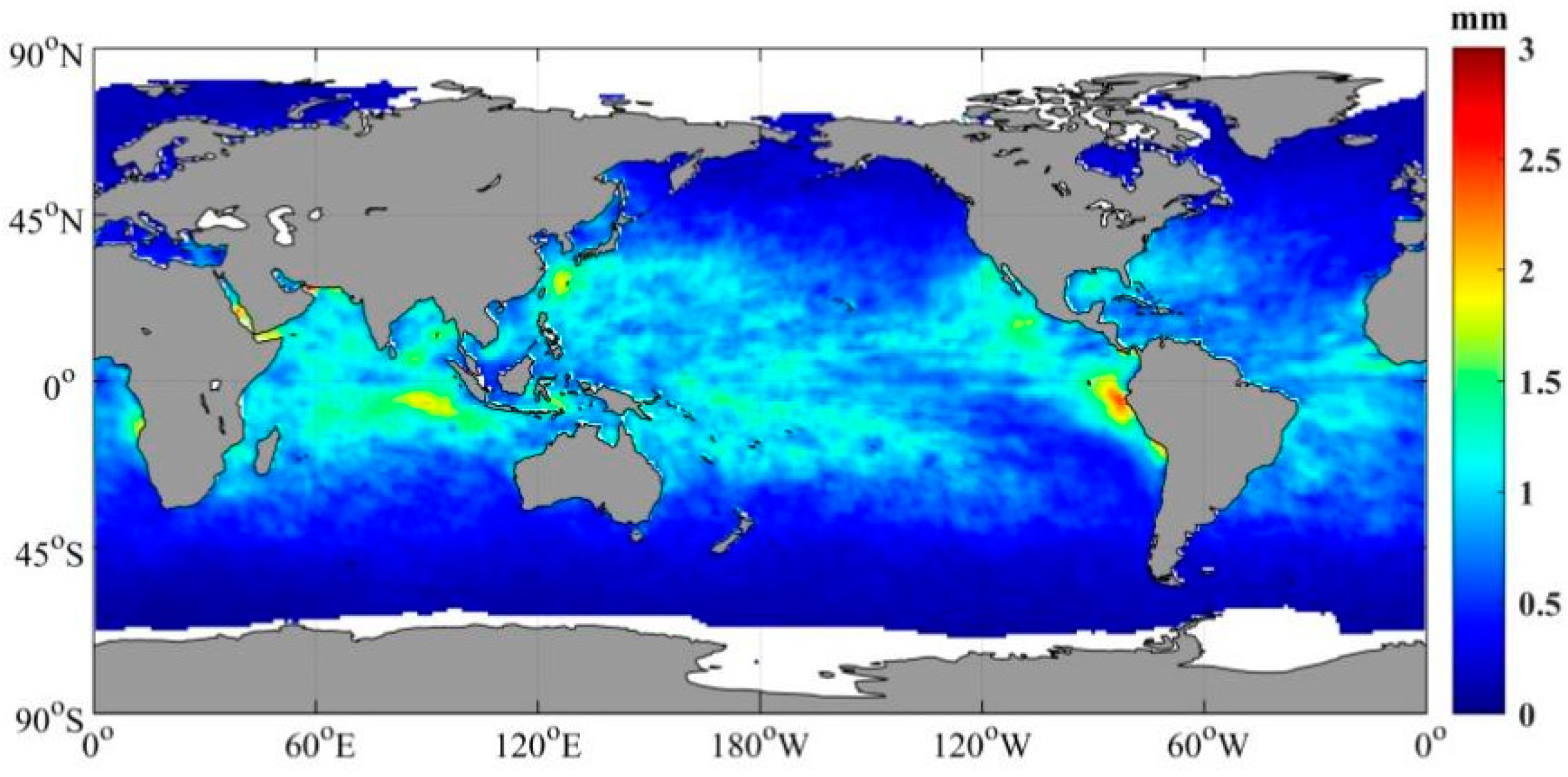
To discuss the global distributions of the monthly standard deviation between this fusion product and the RSS product, the years 2016–2018 were used as an example, and the global map of monthly SD is depicted in Figure 9. The results show that the MAD and SD of the two products are 0.72 mm and 0.98 mm, respectively, and the correlation coefficient (R) is 0.99. As shown in Figure 9, over most global oceans, the standard deviation is mainly less than 1 mm. The largest standard deviation between the two SST products appears in the middle- and low-latitude areas (especially coastal areas), and the maximum occurs in equatorial South America. Thus, it can be concluded that the new gridded product coincides with the RSS product over most global oceans except for some coastal areas. A possible reason for the large standard deviation in these areas is contamination from land and precipitation.
A quantitative comparison with radiosonde data was conducted, and the statistical results are summarized in Table 4. Taking into account the spatial resolution of these two products, the spatial window for the comparison between the fusion product in this paper and the radiosonde data was set to 0.25°, while that of the RSS product was set to 0.5°. Since there were no monthly average radiosonde data, all the radiosonde data in one month were compared with the monthly average of the two satellite-derived water vapor products. As seen from Table 4, the overall error between the two products is very small. The difference is probably caused by the different spatial resolutions of these two water vapor products. The spatial resolution of the fusion product in this study is comparably higher, given that the product here could be characterized with more spatial details of the spatial variations for water vapor.

4. Discussion

The water vapor background used in this paper is from the ERA-Interim reanalysis product. ERA5 data are the most recent global atmospheric reanalysis data produced by the ECMWF; they have been available since 2018 and have succeeded the ERA-Interim [29,30]. In this study, two water vapor fusion products were generated based on the OI algorithm using multisource spaceborne radiometer data and these two kinds of background data in 2018. The two fusion products and the ERA5 reanalysis data were verified by radiosonde data. Table 3 and Table 5 indicate that although the accuracy of ERA5 is relatively low, significant differences in accuracy were not observed between the two products because the background field data were well corrected by the observations of multisource spaceborne radiometers with higher accuracy. Therefore, the ERA5 data can be used to generate fusion data at the early stage or contribute to the ERA-Interim dataset to generate water vapor fusion products.
Note that AMSR-E ceased data services in late 2011 and was succeeded by the AMSR2 and HY-2A microwave radiometers from 2011 to 2015. Therefore, the usage of AMSR2 and HY-2A MR was considered in this study. Among the fusion products in the 13 years of data, the data sources for the period of 2003–2010 were provided by AMSR-E, WindSat, and SSMIS observations. The fusion data in 2011 had a mixture of AMSR-E and HY-2A microwave radiometer data. The AMSR-E data were then replaced by blending the AMSR2 and HY-2A microwave radiometer data for the following period of 2012–2015. To examine the performance of the AMSR2 and HY-2A microwave radiometer data compared with those based on AMSR-E data, a comparative analysis of these two types of water vapor fusion data in 2003–2010 and in 2012–2015 was carried out. From 2003 to 2010, the Bias was 0.60 mm (95% confidence interval: 0.57–0.64 mm), and the SD was 2.70 mm (95% confidence interval: 2.67–2.72 mm). From 2012 to 2015, the Bias was 0.38 mm (95% confidence interval: 0.34–0.42 mm), and the SD was 2.50 mm (95% confidence interval: 2.48–2.53 mm). The error distribution of the two products is shown in Figure 10. Additionally, as suggested in Table 4, the 2012–2015 fusion products are better than the 2003–2010 products in terms of Bias, SD, and RMSE. Therefore, products based on AMSR2 and HY-2A microwave radiometer data generally show better quality than the product based on AMSR-E data.
Compared with the fusion data of 2012–2015, the fusion data of 2016–2018 were not mixed with HY-2A MR data because the HY-2A MR ceased operation after 2016. A comparative analysis of these two types of water vapor fusion data from 2016–2018 and 2012–2015 was carried out. As shown in Figure 11, from 2016 to 2018, the Bias was 0.48 mm (95% confidence interval: 0.42–54 mm), and the standard deviation was 2.49 mm (95% confidence interval: 2.45–2.52 mm). The error distribution of the product in 2016–2018 is shown in Figure 9. A comparison between Figure 10 and Figure 11 suggests that the 2016–2018 fusion products are slightly better than the 2012–2015 products. However, limited differences were observed in the overall accuracy between them.
The remote sensing water vapor fusion product described in this study was generated under the support of the National Key Research and Development Program of China (No. 2016YFA0600102), which is a project of the Ministry of Science and Technology of the People’s Republic of China. The water vapor fusion product is expected to be tested by an independent institute or university later in 2021. Therefore, the merged product should not be released before the assessment; it may be publicly accessed in the near future.

5. Conclusions

Water vapor is an important parameter for studying the global energy balance because it affects ocean radiation, latent heat, and the global water cycle. Analyzing and understanding the spatial and temporal patterns of water vapor are thus crucial for global climate change. In this study, multisource remote sensing water vapor observation data from SSMIS, WindSat, AMSR-E, ASMR2, and HY-2A microwave radiometers were used to develop an extended daily water vapor multisource remote sensing fusion product based on the OI algorithm. The merged daily available product features a high spatial resolution of 0.25° from 2003 to 2018. Then, the accuracy of the produced global ocean atmospheric water vapor fusion products was examined using radiosonde observations. The main conclusions are summarized as follows.
(1)
Over the past 16 years, the RMSE and SD of satellite-derived atmospheric water vapor fusion products in the global ocean combined with radiosonde data are generally better than 3 mm. The Bias shows a positive deviation and is generally smaller than 0.6 mm. MAD is generally better than 2 mm, and R is stronger than 0.98. The errors of remotely sensed water vapor are normally distributed and slightly skewed to positive values from 2003 to 2018.
(2)
The possibility of replacing AMSR-E data with AMSR2 and HY-2A microwave radiometer data was studied after the data service of AMSR-E ceased. The findings showed that the fusion products obtained by combining AMSR2 and HY-2A microwave radiometer data show higher accuracy compared with the water vapor fusion products using AMSR-E data, based on the Bias, SD, and RMSE results. Thus, AMSR2 and HY-2A microwave radiometer data can be used to replace AMSR-E data.

Author Contributions

W.S. developed the OI algorithms and validated the accuracy of the products; J.W. helped to conceive and design the analysis; Y.L. and J.M. contributed to in situ data collection and data processing; Y.Z. and P.W. contributed to remote sensing data collection and data processing. All authors together developed and discussed the manuscript and finally wrote the paper. All authors have read and agreed to the published version of the manuscript.

Funding

The research was funded by the National Key Research and Development Program of China (No. 2016YFA0600102) and the second remote sensing survey of East Indian Ocean environmental parameters (GASI-02-IND-YGST2-04).

Acknowledgments

We thank RSS for providing the SSMIS, WindSat, AMSR-E, and AMSR2 microwave radiometer data for this study; NSOAS for providing the HY-2A L2 microwave radiometer data; and NCDC for providing the radiosonde data.

Conflicts of Interest

The authors declare no conflict of interest.

References

  1. Sherwood, S.C.; Roca, R.; Weckwerth, T.M.; Andronova, N.G. Tropospheric water vapor, convection, and climate. Rev. Geophys. 2010, 48, 2500–2522. [Google Scholar] [CrossRef] [Green Version]
  2. Held, I.M.; Soden, B.J. Water vapor feedback and global warming. Annu. Rev. Energy Environ. 2000, 25, 441–475. [Google Scholar] [CrossRef] [Green Version]
  3. Soden, B.J.; Wetherald, R.T.; Stenchikov, G.L.; Robock, A. Global cooling after the eruption of Mount Pinatubo: A test of climate feedback by water vapor. Science 2002, 296, 727–730. [Google Scholar] [CrossRef] [PubMed] [Green Version]
  4. Liu, Z.; Li, M.; Zhong, W.; Wong, M.S. An approach to evaluate the absolute accuracy of WVR water vapor measurements inferred from multiple water vapor techniques. J. Geodyn. 2013, 72, 86–94. [Google Scholar] [CrossRef]
  5. Miloshevich, L.M.; Vömel, H.; Whiteman, D.N.; Lesht, B.M.; Schmidlin, F.J.; Russo, F. Absolute accuracy of water vapor measurements from six operational radiosonde types launched during AWEX-G and implications for AIRS validation. J. Geophys. Res. Atmos. 2006, 111, 1155–1164. [Google Scholar] [CrossRef] [Green Version]
  6. Bevis, M.; Businger, S.; Chiswell, S.; Herring, T.A.; Anthes, R.A.; Rocken, C.; Ware, R.H. GPS Meteorology: Mapping Zenith Wet Delays onto Precipitable Water. J. Appl. Meteorol. 1994, 33, 379–386. [Google Scholar] [CrossRef]
  7. Liu, Z.; Wong, M.S.; Nichol, J.; Chan, P.W. A multi-sensor study of water vapor from radiosonde, MODIS and AERONET: A case study of Hong Kong. Int. J. Climatol. 2013, 33, 109–120. [Google Scholar] [CrossRef] [Green Version]
  8. Høyer, J.L.; Karagali, I.; Dybkjær, G.; Tonboe, R. Multi sensor validation and error characteristics of Arctic satellite sea surface temperature observations. Remote Sens. Environ. 2012, 121, 335–346. [Google Scholar] [CrossRef]
  9. Wulfmeyer, V.; Bsenberg, J. Ground-Based Differential Absorption Lidar for Water-Vapor Profiling: Assessment of Accuracy, Resolution, and Meteorological Applications. Appl. Opt. 1998, 37, 3825–3844. [Google Scholar] [CrossRef] [PubMed]
  10. Cooney, J. Remote Measurements of Atmospheric Water Vapor Profiles Using the Raman Component of Laser Backscatter. J. Appl. Meteorol. 1970, 9, 182–184. [Google Scholar] [CrossRef] [Green Version]
  11. Huber, P.J. Projection Pursuit. Ann. Stat. 1985, 13, 435–475. [Google Scholar] [CrossRef]
  12. Wang, L.; Jin, W.; He, Y. Infrared and water vapor cloud image fusion using redundant dictionary sparse representation. J. Ningbo Univ. 2014, 3, 32–36. (In Chinese) [Google Scholar]
  13. Liu, K.; Kou, Z. Study of fusion of meteorological satellite infrared image and water vapor image. Hongwai 2013, 34, 8–15. (In Chinese) [Google Scholar]
  14. Wang, J.R.; Manning, W. Near concurrent MIR, SSM/T-2, and SSM/I observations over snow-covered surfaces. Remote Sens. Environ. 2003, 84, 457–470. [Google Scholar] [CrossRef]
  15. Hiroshima, K. Rainfall observation from Tropical Rainfall Measuring Mission (TRMM) satellite. J. Vis. 1999, 2, 93–98. [Google Scholar] [CrossRef]
  16. Wang, K.; Zhang, J.; Wang, C. Objective analysis method of conventional SST data in the Northwest Pacific Ocean. I. Analysis of ten day average ship report data. Mar. Forecast. 2000, 17, 52–59. (In Chinese) [Google Scholar]
  17. Reynolds, R.W.; Marsico, D.C. An improved real-Time global sea surface temperature analysis. J. Clim. 1993, 6, 114–119. [Google Scholar] [CrossRef] [Green Version]
  18. Guan, L.; Kawamura, H. Merging satellite infrared and microwave SSTs: Methodology and evaluation of the new SST. J. Oceanogr. 2004, 60, 905–912. [Google Scholar] [CrossRef]
  19. Reynolds, R.W.; Rayner, N.A.; Smith, T.M.; Wang, W. An improved in situ and satellite SST analysis for climate. J. Clim. 2002, 15, 1609–1625. [Google Scholar] [CrossRef]
  20. Reynolds, R.W.; Smith, T.M. Improved global sea surface temperature analyses using optimum interpolation. J. Clim. 1994, 7, 929–948. [Google Scholar] [CrossRef] [Green Version]
  21. Reynolds, R.W.; Smith, T.M.; Liu, C.; Chelton, D.B.; Casey, K.S.; Schlax, M.G. Daily high-resolution-blended analyses for sea surface temperature. J. Clim. 2007, 20, 5473–5496. [Google Scholar] [CrossRef]
  22. Sun, W.; Wang, J.; Zhang, J.; Ma, Y.; Meng, J.; Yang, L.; Miao, J. A new global gridded sea surface temperature product constructed from infrared and microwave radiometer data using the optimum interpolation method. Acta Oceanol. Sin. 2018, 37, 41–49. [Google Scholar] [CrossRef]
  23. Zabolotskikh, E.; Mitnik, L.; Reul, N.; Chapron, B. New possibilities for geophysical parameter retrievals opened by GCOM-W1 AMSR2[C] Microwave Radiometry and Remote Sensing of the Environment. IEEE J. Sel. Top. Appl. Earth Obs. Remote Sens. 2014, 8, 161–166. [Google Scholar]
  24. Jiang, X.; Lin, M.; Liu, J.; Zhang, Y.; Xie, X.; Peng, H.; Zhou, W. The HY-2 satellite and its preliminary assessment. Int. J. Digit. Earth 2012, 5, 266–281. [Google Scholar] [CrossRef]
  25. Team of GCOM Project. GCOM-W1 “SHIZUKU” Data Users Handbook, AMSR2 Products, 1st ed.; Japan Aerospace Exploration Agency: Tokyo, Japan, 2013; pp. 4-38–4-39. [Google Scholar]
  26. Wenqing, T.; Yueh, S.H.; Fore, A.G.; Hayashi, A.; Lee, T.; Lagerloef, G. Uncertainty of Aquarius sea surface salinity retrieved under rainy conditions and its implication on the water cycle study. J. Geophys. Res. Oceans 2014, 119, 4821–4839. [Google Scholar]
  27. Martin, M.; Dash, P.; Ignatov, A.; Banzon, V.; Beggs, H.; Brasnett, B.; Gayula, J.-F.; Cummings, J.; Donlon, C.; Gentemann, C. Group for High Resolution Sea Surface temperature (GHRSST) analysis fields inter-comparisons. Part 1: A GHRSST multi-product ensemble (GMPE). Deep Sea Research Part II. Top. Stud. Oceanogr. 2012, 77, 21–30. [Google Scholar] [CrossRef]
  28. Kako, S.; Isobe, A.; Kubota, M. High-resolution ASCAT wind vector data set gridded by applying an optimum interpolation method to the global ocean. J. Geophys. Res. Atmos. 2011, 116, 23107. [Google Scholar] [CrossRef] [Green Version]
  29. Hoffmann, L.; Günther, G.; Li, D.; Stein, O.; Wu, X.; Griessbach, S.; Heng, Y.; Konopka, P.; Müller, R.; Vogel, B.; et al. From ERA-Interim to ERA5: The considerable impact of ECMWF’s next-generation reanalysis on Lagrangian transport simulations, Atmos. Chem. Phys. 2019, 19, 3097–3124. [Google Scholar] [CrossRef] [Green Version]
  30. Wang, S.; Xu, T.; Nie, W.; Jiang, C.; Yang, Y.; Fang, Z.; Li, M.; Zhang, Z. Evaluation of Precipitable Water Vapor from Five Reanalysis Products with Ground-Based GNSS Observations. Remote Sens. 2020, 12, 1817. [Google Scholar] [CrossRef]
Figure 1. Technical process of the water vapor fusion product.
Remotesensing 13 02402 g001
Figure 2. Locations of the radiosonde stations. The red dots indicate the positions of the radiosondes.
Remotesensing 13 02402 g002
Figure 3. Implementation mechanism of the fusion algorithm for water vapor. A new 0.25° background field (Bk) was reconstructed using the bilinear interpolation method. Then, (OiBi) was calculated using the radiometer water vapor and new background.
Remotesensing 13 02402 g003
Figure 4. Comparison of water vapor fusion data and single spaceborne radiometer data on 1 January 2018. The white areas in the middle and low latitudes in Figure 4 are areas that cannot be observed by satellites. The observation ability of spaceborne radiometers in polar regions is poor due to the influence of sea ice.
Remotesensing 13 02402 g004
Figure 5. Daily coverage of multisource spaceborne radiometer water vapor data of 2018. The data coverage of the microwave radiometer is defined as the proportion of the effective observation data grid to the global ocean grid.
Remotesensing 13 02402 g005
Figure 6. Number of effective observations of multisource spaceborne radiometer water vapor data of 2018. This figure is expressed using the daily average data calculated by using the effective water vapor observation data of spaceborne radiometers in 2018.
Remotesensing 13 02402 g006
Figure 7. Comparison of the water vapor fusion products with radiosonde data from 2003 to 2018. Error distributions of the fusion product in 2003–2018 are shown in the graph on the left. The right picture shows the scatter distribution of water vapor fusion data and radiosonde data.
Remotesensing 13 02402 g007
Figure 8. Taylor diagram drawn using the fusion product in 2018. The red point represents the fusion product.
Remotesensing 13 02402 g008
Figure 9. Global distributions of the monthly standard deviation between the fusion product and RSS product during 2016–2018. First, the monthly water vapor of each month from 2016 to 2018 was obtained by using the fused water vapor data. Then, the calculated monthly water vapor data were compared with the monthly water vapor data of the RSS. Finally, the standard deviation was obtained by using the monthly water vapor data of 36 months.
Remotesensing 13 02402 g009
Figure 10. Error comparison of fusion products using different data sources.
Remotesensing 13 02402 g010
Figure 11. Error distributions of the fusion product in 2016–2018.
Remotesensing 13 02402 g011
Table 1. Satellite radiometer remote sensing data of water vapor.
SensorsResolutionData Time Period UsedSpatial Coverage
AMSR-EDaily/25 kmJanuary 2003–October 2011Global ocean
AMSR2Daily/25 kmJuly 2012–December 2018Global ocean
WindSatDaily/25 kmJanuary 2003–December 2018Global ocean
SSMISDaily/25 kmJanuary 2003–December 2018Global ocean
HY-2A MRSwath/97 kmOctober 2011–December 2015Global ocean
SSMIS includes data from the F16, F17 and F18 satellites.
Table 2. Statistics on the precision of global ocean water vapor fusion products.
YearData MatchesBias (mm)MAD (mm)SD (mm)RMSE (mm)R
200323650.502.072.792.840.99
200429610.521.942.602.650.99
200529160.872.042.662.800.99
200627710.992.523.173.330.98
200726160.362.243.023.040.99
200828470.482.042.782.830.98
200930360.661.802.432.530.99
201034900.431.532.112.150.99
201130980.411.842.672.700.99
201230140.241.562.152.160.99
201329690.301.722.422.440.99
201429980.571.872.522.590.98
201528700.371.962.702.730.98
201627550.301.852.602.620.99
201725200.541.782.512.570.99
201819650.661.652.272.360.99
Table 3. Statistics of ERA-Interim global ocean water vapor background precision in 2016–2018.
YearBias (mm)MAD (mm)SD (mm)RMSE (mm)R
20160.641.942.862.930.99
20170.621.822.692.760.99
20180.871.963.173.290.99
Table 4. Accuracy comparison between the fusion product and RSS product from 2016 to 2018. The monthly water vapor of each month from 2016 to 2018 was obtained using the fusion water vapor data.
DataYearMAD (mm)SD (mm)RMSE (mm)R
Fusion product20161.582.302.300.99
Fusion product20171.693.893.890.97
Fusion product20181.672.462.480.99
RSS product20161.612.382.390.99
RSS product20171.743.853.860.97
RSS product20181.732.532.580.99
Table 5. Accuracy comparison of fusion products using different background fields in 2018 (including the accuracy of ERA5).
DataBias (mm)MAD (mm)SD (mm)RMSE (mm) R
Fusion product using ERA-interim0.661.652.272.360.99
Fusion product using ERA50.721.682.282.390.99
ERA5 reanalysis1.082.123.443.600.99
Publisher’s Note: MDPI stays neutral with regard to jurisdictional claims in published maps and institutional affiliations.