Abstract
Noise radars employ random waveforms in their transmission as compared to traditional radars. Considered as enhanced Low Probability of Intercept (LPI) radars, they are resilient to interference and jamming and less vulnerable to adversarial exploitation than conventional radars. At its simplest, using a random waveform such as bandpass Gaussian noise as a probing signal provides limited radar performance. After a concise review of a particular noise radar architecture and related correlation processing, this paper justifies the rationale for having synthetic (tailored) noise waveforms and proposes the Combined Spectral Shaping and Peak-to-Average Power Reduction (COSPAR) algorithm, which can be utilized for synthesizing noise-like sequences with a Taylor-shaped spectrum under correlation sidelobe level constraints and assigned Peak-to-Average-Power-Ratio (PAPR). Additionally, the Spectral Kurtosis measure is proposed to evaluate the LPI property of waveforms, and experimental results from field trials are reported.
1. Introduction
Noise radars transmit random signals, as opposed to traditional radars having deterministic waveforms. This randomness provides advantages in many ways both for the civil and military fields. In civilian applications such as automotive radar or marine navigation, noise radars mitigate mutual interference [1] caused by the density of radars working in the same area and sharing the same spectrum. From a military perspective, noise radar possesses good Electronic Protection (EP) attributes with strong immunity against adversary Electronic Attacks (EA), e.g., jammers, and allows Low Probability of Intercept (LPI) operation against Electronic Support Measure (ESM) receivers due to the unpredictable and random nature of its signals [2].
The use of random signals for detecting objects dates back to the late 19th and early 20th centuries. In 1897, Alexandr S. Popov used random pulses in his radio experiments and reported that ship detection was possible in a bistatic configuration [3], and this was followed by Christian Huelsmeyer in 1904, where he used noise pulses of a spark generator to detect the presence of ships with his device named Telemobiloscope, also known as the “radar precursor” [4,5]. However, at that time, the technology was immature and the sensing of objects was based on a simple radio detector (called “coherer”) rather than the coherent reception and correlation of signals.
The pioneering work on the coherent reception of random signals was performed by R. Bourret in 1957 [6]. His paper is considered to be the first paper on coherent radar using noise signals. It was followed by B. M. Horton in 1959, who described the theory of using random noise signal in detail to measure the object range [7].
Much of the early work included physical delay lines to match the delay of the reference signal to the object range and thus could only offer limited range. However, this technique has long been of interest due to the fact that intercept receivers observe only noise from the transmitting radar. Moreover, the nonrepetitive nature of transmissions would remove range and Doppler ambiguities on reception. However, due to the technical difficulties and lack of noise generating apparatus, the noise radar concept was not quite realizable by radar engineers at that time. In the late 20th century, with the technological advances in microwave and digital electronics, there was a major shift from analog to digital and it became possible to generate random signals and perform correlation processing fully digitally. Over the past three decades, there has been a considerable interest in noise radar technology and significant progress has been made by research communities [8,9,10].
Random signals are realizations of a random process either generated physically by an analog source or digitally by a pseudo random noise generator. Once a realization of this random process is employed as the modulating code, the radar knows what has been transmitted and so can detect its presence in the received signal via matched filtering. The theory of matched filter tells us that noise radars can have similar performance merits in terms of range and Doppler resolution as conventional radars, i.e., the range resolution depends on signal bandwidth, and the Doppler resolution depends on coherent integration time. Another incentive for researchers has been its appropriateness for covert radar as stealth requirements can be met by low power and long duty-cycle noise waveforms.
Noise radars have many advantages compared to conventional radars [11]. The distinctive features of noise radars can be listed as follows:
- (i)
- It is impractical for an adversary to intercept and exploit the transmitted signal due to the unpredictable and random nature of noise signals.
- (ii)
- The mitigation of mutual interference among radars sharing the same spectral band due to the (quasi) orthogonality of signals.
- (iii)
- The thumbtack shape of its Ambiguity Function allows high resolution both in range and Doppler space.
Despite these advantages, noise radar comes at a cost of computational burden as it requires a large bandwidth for processing wideband noise waveforms on return and fast digitizers to provide a sufficient sampling rate compared to traditional FMCW radars.
Noise radars can operate either in pulsed or continuous wave (CW) mode depending on the application. However, the use of CW emissions best matches the LPI properties of the noise signal because of the absence of edge modulations in the signal. No matter which emission regime is employed, the choice of transmit waveform has a significant effect on the radar performance. Using a random waveform such as a bandpass Gaussian noise (zero–mean and unit-variance) provides limited dynamic range (as shown later in Section 1.3) in radar sensitivity due to its sidelobe level and degrades radar detection performance. Therefore, noise radars require synthetic waveforms tailored at will to provide adequate resolution, dynamic range and detection performance.
The objective of this article is to introduce the reader to a particular type of waveform which can improve the dynamic range while boosting LPI characteristics and ensuring orthogonality. The remainder of this article is organized as follows. In Section 1 (1.2–1.4), we introduce the reader to the particular continuous noise radar architecture that we are interested in and its related correlation processing implementation. In the ensuing parts, we address the dynamic range problem, correlation sidelobes and leakage effects, and Peak-to-Average-Power-Ratio (PAPR) considerations, and next, we provide a clear rationale for the usage of tailored noise waveforms. In Section 2, we present the steps of the novel Combined Spectral Shaping and Peak-to-Average Power Reduction (COSPAR) waveform generation method along with a cyclic PAPR reduction procedure. In Section 3, we provide a discussion on the range resolution and mainlobe broadening for COSPAR signals. Then, we show the mutual orthogonality of COSPAR signals in Section 4. Next, the Ambiguity Function and Doppler sensitivity of COSPAR signals are compared with those of a typical LFM signal in Section 5. After that, we propose the Spectral Kurtosis (SK) measure to assess the LPI characteristics of signals and compare the time–frequency distributions of COSPAR and LFM waveforms in Section 6. In Section 7, we report experimental results obtained from the field trials. Finally, the article ends with concluding remarks in Section 8.
1.1. Noise Radar Architecture
Before we proceed to tailored noise waveform design, we find it helpful to introduce the reader to the general system architecture for noise radar technology. This will help the reader better understand the concept of noise radar technology and its associated signal processing.
Noise radar emits noise signals, which are generated either by analog noise sources (temperature-controlled resistors, Zener diodes, gas discharge tubes …) or digital pseudo random noise generators. Since analog noise sources provide limited performance in terms of resolution and dynamic range, in this work we are solely interested in digital waveforms generated synthetically on computing devices such as computers, DSPs or FPGAs. Thus, we particularly refer to a typical noise radar architecture, shown in Figure 1, with collocated transmit and receive antennas. In this architecture, the waveform is generated or stored in a digital device and it is fed to the transmitter by the Digital-to-Analog Converter. It should be noted that analog filters and signal conditioning components are omitted in this simplified block diagram. Interested readers may refer to [12] for other types of architectures.
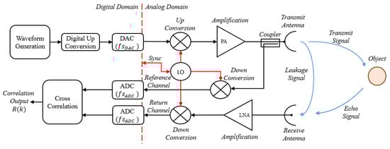
Figure 1.
Noise radar block diagram.
In Figure 1, the complex baseband signal (noise waveform) is first generated and then up-sampled and digitally up-converted (complex-to-real conversion) to the radar intermediate frequency (IF) band. Next, the digital real IF band signal is driven into the Digital-to-Analog Converter (DAC) at DAC sampling rate . In the analog domain, the signal is first up-converted by a mixer to the RF band, then amplified by the power amplifier (PA) and finally transmitted through the antenna. A coherent local oscillator (LO) provides the RF signal required for up and down conversion. During transmission, the replica of the transmit signal going into the antenna is tapped by an RF coupler and down-converted back into the IF band. This signal is used as the matching template in the correlation processing, hence termed as the “reference signal”. Alternatively, the digital version of the transmit signal that is stored in the hardware can be used for correlation. However, the design shown here is notedly preferred in order to include the nonlinear effects of the transmitter (i.e., imposed on the transmit signal) in the correlation processing at the expense of an additional downconverter stage. At the receive antenna, the weak echo signal, which reflects back from the object that we are interested in detecting, is first amplified by a low noise amplifier in the receiver and then down-converted into the IF band. As its name implies, this signal is called the “return signal” (or “surveillance signal”). Both reference and return signals are sampled by the Analog-to-Digital Converters (ADCs) at ADC sampling rate and cross-correlation is computed digitally in the hardware.
In this architecture, it is customary to generate the complex baseband signal at sampling rate and set the IF band within the 3rd Nyquist zone of ADCs ( to). In this scheme, the ADCs subsample the incoming reference and return signals and then the spectrum folds over to the 1st Nyquist zone, obviating the need for an additional digital downconverter before the cross-correlation processing.
The noise radar described here transmits and receives simultaneously and this leads to an unavoidable leakage into the receiver due to the coupling of collocated antennas. This leakage is very important in noise radar applications and as such it has an effect on the dynamic range, which will be discussed later in Section 1.2. Moreover, the noise radar utilizes a continuous wave (CW) emission, granting covertness with an absence of pulse edges (which can be easily detected by ESM receivers) in its emissions. The continuous emission leads to a continuous processing of return signals, necessitating fast and low latency signal processing in the receiver.
1.2. Correlation Processing and Its Implementation in Spectral Domain
In noise radar, the fundamental way of calculating the cross-correlation is performed by matched filtering. This procedure is also called “pulse compression” as it compresses the signal energy into a much narrower correlation mainlobe than the duration of the signal. The matched filter is known as the optimal linear filter for maximizing the signal-to-noise ratio (SNR) when the received signal is contaminated by additive white noise [13]. For this reason, matched filters are widely used in radar, in which a signal known a priori is transmitted, and the return signal reflected from objects is analyzed for matching copies of the transmit signal.
In signal processing, a matched filter is derived by correlating a template signal (delayed and possibly Doppler compensated) with an unknown signal to search for the existence of the template signal in the unknown signal. This is identical to convolving the received signal with a conjugated time-reversed version of the transmit signal. In this respect, we define the continuous time autocorrelation function (ACF) of signal as the following:
In practice, considering the discrete time case, the waveform is both time and band limited. Therefore, from the waveform point of view, there could be two options for the correlation processing. One is the periodic correlation, which assumes the waveform is periodic and thus the correlation is calculated via cyclic convolution. The other one assumes the signal is aperiodic and therefore the correlation is calculated via linear convolution [14]. In our work, we opt for the periodic correlation due to the non-interlaced reception of signals dictated by the CW operation of noise radar.
For the ease of digital implementation, given the discrete sequence , we prefer to use the frequency domain calculation of correlation , which is defined as:
where , , ◦ and denote the Discrete Fourier Transform (DFT), the Inverse Discrete Fourier Transform (IDFT), the Hadamard Product and Complex Conjugate operator, respectively. The sequence is the sampled version of the ACF where and is the sampling period. DFT and IDFTs are obtained by Fast Fourier Transform (FFT) usually available on digital hardware.
A digital hardware implementation for a periodic correlator is shown as a block diagram in Figure 2. In the block diagram, all arithmetic operations including complex conjugation and complex multiplication are performed on digital hardware such as FPGA. The Hilbert Transform is implemented as an FIR filter structure and FFT/IFFTs are implemented by Radix-2 or Radix-4 decompositions for the calculation of DFT and IDFT, respectively. Such an example implementation is shown in [15].
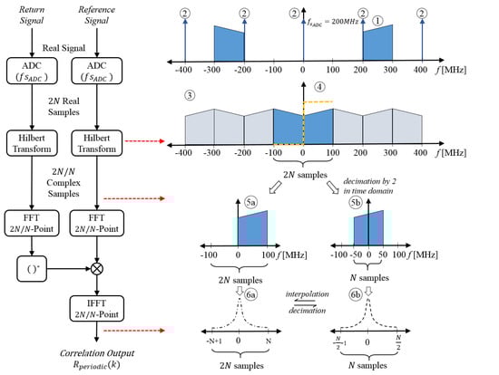
Figure 2.
Periodic correlation processing in spectral domain. (1) Spectrum of the “Low IF” signal. (2) Spectrum of the sampling comb (arbitrary units) at . (3) Their convolution and the low frequency alias ( samples) of the IF signal. (4) Transfer function of the Hilbert filter. (5a/b) Resulting low-pass component with significant samples ( samples for the decimated case, i.e., I and Q components) in both frequency and time. (6a/b) Periodic cross-correlation result with samples ( samples for the decimated case).
In Figure 2, we also illustrate the calculation of a periodic autocorrelation of a signal and show the power spectrum at each step during low IF sampling and Hilbert filtering. Here, we consider an exemplary analog IF band (200–300 MHz) signal is being injected to both ADCs where the sampling rate is . The subsampling process down-converts the signal from the 3rd Nyquist zone into baseband (DC-100 MHz), generating a low-pass alias of the IF signal, and then the Hilbert Transform is applied to obtain the analytic form of the signal in order to keep phase information for the subsequent Doppler processing. After that, the spectral domain periodic correlation is calculated as in Equation (2). Alternatively, one can down-sample the complex valued output of the Hilbert Transform by half to remove the negative frequency components from the spectrum and to obtain a decimated autocorrelation with a lower number of resource usage for FFTs in digital hardware (see Figure 2).
That being said, we note that all synthetic waveforms shall be generated in conjunction with its digital correlator, i.e., the samples of complex baseband signal should be generated at the sampling rate (e.g., ) at which its correlation is computed in the digital backend. This eliminates the distortion in the ACF sidelobes caused by the sampling rate mismatches.
1.3. Dynamic Range of Noise Radar
Having shown the correlation processing implementation, we wish to discuss the dynamic range requirement for noise radars. There are two important factors affecting the receiver sensitivity, i.e., the choice of waveform and the system noise bandwidth.
1.3.1. Random Sidelobe Modulations of Noise Signals
In noise radar, when using standard bandpass Gaussian noise as a probing waveform, the correlation processing of noise signals of duration and bandwidth generates “random sidelobe modulations” (sometimes called “range sidelobes”) whose mean level “” is equivalent to the product below the correlation mainlobe peak [12]:
These “random sidelobe modulations” cover the whole range swath and thus mask the visibility of weak targets with low radar cross section (RCS), i.e., not only nearby targets but also those at a great distance. This is also known as the “masking effect”.
On the other hand, considering the unavoidable leakage signal due to antenna coupling, the correlation processing generates a target at zero distance, the range sidelobes of which roughly define the dynamic range lower bound of the noise radar. This leakage signal can be regarded as the largest signal (in terms of power) going into the receiver and therefore cross-correlation calculations are normalized with respect to the peak response of the leakage signal. Additionally, the receiver gain is adjusted carefully such that the leakage signal does not saturate the receiver.
1.3.2. Receiver Noise Considerations
Aside from the range sidelobes of the leakage signal, the cross-correlation of the reference signal with the internal noise of the receiver shall be taken into consideration. Assuming a receiver gain and a receiver noise figure , then the receiver noise power at the input of ADC is given as the following:
where K is the Boltzmann constant, is the system temperature in and is the receiver bandwidth. Having an antenna isolation level , then the leakage signal power at the input of ADC is:
where is the signal power transmitted from the antenna. After that, the signal-to-noise ratio due to the leakage signal and receiver noise can be defined as the following:
Neglecting the quantization noise due to the fixed wordlength of ADCs, finally the noise floor after correlation processing is defined as:
Assuming a positive valued (), this means that when using a standard Gaussian noise signal as the transmission signal, the dynamic range is limited by the random sidelobe modulations of the leakage signal rather than the actual noise floor due to system internal noise (). As a result, an undesirable sensitivity loss equivalent to (in occurs. To eliminate the SNR loss, the range sidelobes of the noise waveforms shall be lowered at least to the following sidelobe level (:
As a comparison, the dynamic ranges are shown on one-sided correlation plots (up to lag index 4000) in Figure 3a,b for two cases where bandpass Gaussian noise and tailored noise signals having the same bandwidth and duration () are used, respectively.
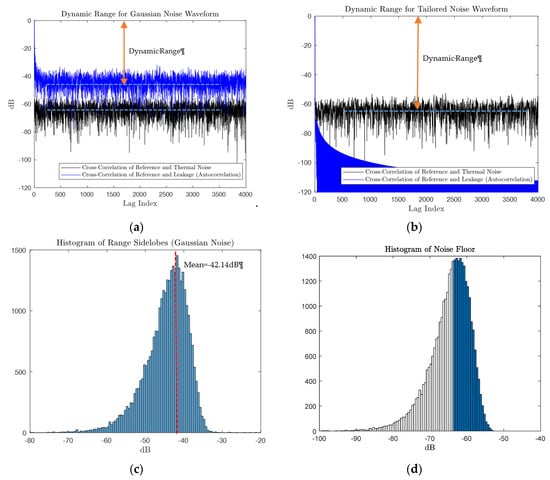
Considering a 100 mW (20 dBm) transmit power with an antenna isolation level of 90 dB gives a leakage power level of −70 dBm at the receiver antenna. Assuming a receiver bandwidth of 100 MHz and a system temperature of 273 , then the thermal noise power is equal to −93.97 dBm. When a typical receiver noise figure of 4 dB is applied, then the leakage to noise power ratio at the ADC input is:
For both cases, the cross-correlation of the reference signal and thermal noise would give us a mean noise floor of:
which is consistent with the histogram shown in Figure 3d. In the case of the Gaussian noise waveform, the dynamic range of the radar is limited by the range sidelobes of the transmit signal itself, which has a mean level of −42.14 dB, as shown in Figure 3c. On the other hand, when a tailored noise waveform is used such as a COSPAR waveform with −70 dB peak sidelobe level, then the range sidelobes are far lower than and as a result, the dynamic range is limited by the system thermal noise floor rather than the waveform’s range sidelobes. The latter case is desirable in noise radar and the example provided here explains the dynamic range issue in noise radar and the need for controlling the range sidelobes of noise waveforms, and this motivates us for the generation of tailored waveforms with desired correlation sidelobe properties.
1.4. Peak-to-Average Power Ratio
Another important metric in noise radar is the Peak-to-Average Power Ratio (PAPR) of signals. The PAPR of radiated signal here represented by its discrete samples is defined as:
where is the sample number with being the sampling frequency.
Signals with constant amplitude envelope (termed as “unimodular”) have a PAPR level of 1, which makes them ideally power efficient. Exemplary waveforms belonging to this group can be listed as LFM, Barker and Polyphase codes. Such signals can drive the power amplifiers near saturation, thereby allowing power maximization during transmission. Any deviation from the unitary amplitude level leads to an energy loss in the correlation mainlobe, i.e., lowering the peak response level. This can be regarded as loss, causing a degradation in the detection performance. This inevitable loss is defined as:
The versus various PAPR values is shown in Figure 4. In this respect, having a PAPR < 2 is tolerable in noise radar applications without substantial degradation in detection performance (dB).
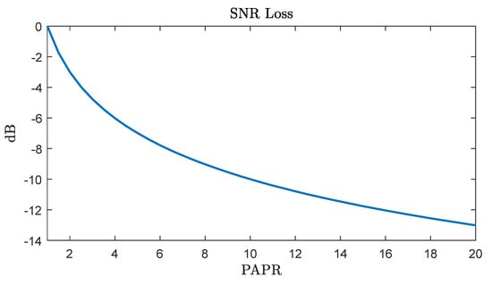
Figure 4.
SNR loss versus PAPR.
Aside from SNR loss, signals with non-constant envelope are vulnerable to nonlinear distortion effects of amplifiers such as clipping, which impairs the good correlation properties of radiated signals. Therefore, signals with large PAPR necessitate highly linear converters, and amplifiers with wide dynamic range thus bring additional costs for radar system designers.
2. The COSPAR (Combined Spectral Shaping and Peak-to-Average Power Ratio Reduction) Method: General Description
Having shown the particular noise radar architecture and the fundamental periodic correlation processing scheme, with some important aspects related to noise radar technology, here we propose a noise waveform generation method for controlling sidelobes and an accompanying PAPR reduction technique for SNR maximization and linear amplifier operation. The noise waveform generation method described here is based on having a good spectral shape (e.g., a Taylor window function), giving an opportunity to control the sidelobes in its transformed domain.
It is well known by the Wiener–Khinchin theorem that the Power Spectral Density (PSD) of a signal is the Fourier transform of its Auto-Correlation Function (ACF). Thus, the PSD and ACF form a Fourier pair. Using this relation, if one can find a good spectral shape (square root of PSD) with desired ACF sidelobe properties, then adding an arbitrary phase spectrum to that spectral shape and taking the inverse Fourier transform leads to a single realization of a noise-like waveform. Using this technique, it is possible to generate infinitely many waveforms having the same PSD and ACF by randomizing the phase term for signal spectra at each realization. In this respect, we resort to the Taylor window function for the spectral shape synthesis and after each realization we apply our proposed PAPR reduction method. An illustration of the procedure is shown in Figure 5 and the steps of the COSPAR method are explained in the following subsections.
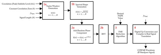
Figure 5.
Block diagram of COSPAR waveform synthesis method.
2.1. Step I: Spectral Shape Synthesis
We begin the COSPAR procedure by constructing the spectral shape, which will provide us the desired correlation properties. For this purpose, we refer to window functions where designers can adjust the coefficients or window weights to make tradeoffs between mainlobe width, peak sidelobe level and sidelobe fall-off rate parameters.
Window functions are widely used in digital signal processing for controlling undesirable sidelobes or suppressing spectral leakage and Gibbs oscillations. Also called taper or apodization functions, researchers have developed various window functions throughout the years to achieve certain sidelobe properties. Thus, there exists an extensive literature on window functions and they are widely used in applications such as spectral analysis, beamforming and antenna design [16,17].
In the COSPAR procedure, we resort to the Taylor window function in particular [18]. Compared to other window functions, the Taylor window offers several advantages for noise radar waveform desigi
- (i)
- Peak sidelobe level (PSL) can be specified according to desired correlation PSL dictated by the radar design.
- (ii)
- Near-in sidelobes can be specified for the desired range where constant sidelobe response is required.
- (iii)
- Tradeoff between mainlobe width and sidelobes does not have a substantial effect on the radar resolution. The mild broadening of the mainlobe is discussed in Section 3.
- (iv)
- The good roll-off factor and monotonic decrease in the sidelobes beyond the constant sidelobe zone allow the visibility of weak targets at far range.
In fact, Taylor windows are similar to the Chebyshev window, which is known to have the narrowest mainlobe for a given sidelobe level; however, the Chebyshev window comes at a cost such that flat equiripple sidelobes lead to edge discontinuity in the window function (in our case, the spectral shape), which is not desirable for LPI radar operation. Avoiding edge discontinuity, the Taylor window allows us to make tradeoffs between the sidelobe level and the mainlobe width.
Having discussed the good features of the Taylor window, we finally define a parameterized discrete Taylor window [19] which is specified by three parameters: and , where:
- (i)
- is the number of samples (coefficients) in the Taylor window;
- (ii)
- is the number of nearly constant-level sidelobes adjacent to the mainlobe;
- (iii)
- is the peak sidelobe level (in dB) relative to the mainlobe peak.
The -length Taylor window is computed as the sum of a constant and cosine functions according to:
The cosine weights in Equation (11) are determined by:
where
An exemplary discrete Taylor window with parameters and and its Fourier transform are shown in Figure 6. After the generation of the Taylor window , we use it to generate the spectral shape function defined by for .
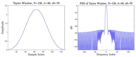
Figure 6.
Taylor window and its power spectral density.
2.2. Step II: Signal Synthesis
Having synthesized the spectral shape according to the desired level of correlation sidelobes in Step I, we have degrees of freedom, i.e., to choose an arbitrary phase to construct the signal spectrum , defined as:
where is a random vector on with a probability density function . Then, the baseband complex signal is obtained by taking the Inverse Fourier Transform of .
An example will illustrate the COSPAR waveform generation procedure up to this step. Later in Section 2.2 we will show how to reduce the PAPR of the synthesized signal by optimizing phase samples of the signal spectrum.
Example 1
As a demonstration of the design procedure, let it be desired to create a −60 dB sidelobe level ACF pattern with nearly constant near-in sidelobes of 20 (). We wish to transmit and receive a radar waveform with a bandwidth of 100 MHz and a duration of . Assuming an ADC sampling rate of 200 MSPS in the receiver, then this corresponds to a total number of 32,768 samples. Since the signal is real-valued, its power spectrum is symmetric and therefore we only consider designing the positive side of the power spectrum. Hence, our waveform design task boils down to a synthesis of a complex sequence of length 16,384. This complex sequence is in fact the complex envelope representation of the real-valued radar waveform.
Having specified the parameters, we synthesize our spectral shape using Equation (11). The constant-level sidelobe zone specified by corresponds to a distance m, which is defined by where is the speed of light.
Once we generate the Taylor-shaped magnitude spectrum, we append a random phase vector to the modulus of the spectrum and then take the IDFT, which leads to a single realization of the noise signal shown in Figure 7a. The Taylor-shaped power spectrum and the one-sided autocorrelation of the noise signal are shown in Figure 7b,c, respectively. We note that the signal has a PAPR = 9.13, which could be regarded considerably high for linear noise radar operation.
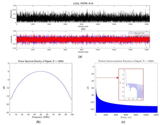
Figure 7.
(a) COSPAR signal. (b) Normalized power spectral density of COSPAR signal. (c) Normalized one-sided autocorrelation of COSPAR signal.
2.3. Step III: PAPR Reduction Procedure
Post synthesis, the waveforms look like noise as they do not possess a deterministic structure neither in envelope nor in quadrature and in-phase components. Furthermore, randomizing the phase term of the modulus of the Taylor-shaped spectrum in Step II, let us generate an infinite number of distinct noise waveforms with different time–frequency distributions at each realization. However, in terms of power efficiency, the waveforms synthesized with this method are far lower than classical waveforms such as LFM or NLFM, which have constant modulus, i.e., unimodular envelope, over the extent of the signal. By experiment, signals generated via COSPAR without the PAPR reduction step tend to have a PAPR value around 8–11.
Now, the question is “how to reduce PAPR without affecting the PSD and ACF envelope of the signal?” Many PAPR reduction algorithms exist in the literature for wireless communication, especially for OFDM signals [20,21]. However, these algorithms are not directly applicable to radar signals as they are developed to maintain the information content (i.e., symbols) of the communication signal while optimizing the code. For radar signals, there exists an alternating projection-based algorithm [22], which provides a suitable and efficient solution to force the signal to obtain a desired PAPR. This algorithm seeks a tight frame given a prescribed structure (e.g., PAPR, norm) by projecting a frame which is described by its spectrum. The solution is found between the intersection of the vectors satisfying the given PAPR constraint and the vectors having certain spectral constraints. The downside of this approach is that the final solution has a slightly transformed spectrum and thus the good sidelobe properties of ACF are degraded. For this reason, we opt not to use this approach and, instead, we propose a novel method based on alternating time–frequency domain projection. In our method, we treat the problem analogous to the Phase Retrieval problem [23] and our procedure follows the steps for the well-known Gerchberg–Saxton algorithm [24], which is widely used for recovering the underlying complex signal (e.g., image) from Fourier magnitude measurements. In this algorithm, the signal is projected onto Fourier and object domains iteratively until a specified criterion is met while Fourier and object domain constraints are applied at each domain, respectively. The procedure is illustrated in Figure 8.
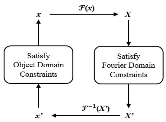
Figure 8.
Gerchberg–Saxton phase retrieval algorithm.
In our method, we first initialize the vector with the sequence generated at Step II. Next, we apply a time domain constraint (i.e., clipping the overshooting sample) and then project it to the frequency domain whenever clipping occurs on a sample by sample basis. In the frequency domain, we apply the spectral constraint (i.e., force it to have the magnitude spectrum obtained in Step I while keeping the modified phase spectrum) and then we project it back to the time domain. The projection is performed via FFT/IFFT operations and this alternation is repeated for each overshooting sample in turn in the entire vector. This iteration continues until a desired stop criterion (e.g., PAPR value or PAPR improvement) is reached at the end of each pass over the entire vector. It should be noted that this cyclic iteration proceeds by one sample-by-one sample for each overshooting sample in order to minimize the regrowth of overshoot and to accelerate the convergence. However, the stop criterion is checked only once at each time the end of the sequence is reached. It is observed that the proposed procedure reduces PAPR at each pass over the entire frame and it converges to a desired PAR level. Consequently, nearly unitary () signals are achievable without altering the PSD and ACF. We provide the algorithm definition for the PAPR reduction procedure in Algorithm 1 and an example will illustrate the procedure next.
Example 2
We initialize the PAPR reduction algorithm with which is the sequence obtained in . The initial PAPR of the sequence is evaluated as and we set our target PAPR to . It has been shown that the PAPR value drops quickly below after several passes. As the PAPR value gets close to the target PAPR, improvement decreases and the rate of convergence slows down. Thus, it is preferable to stop the algorithm according to an improvement factor () rather than satisfying an exact PAPR value condition to cut down runtime. The convergence plot is shown in Figure 9.
| Algorithm1. PAPR reduction procedure. |
| Initialization • Initialize having a known spectral shape (e.g., Taylor window) or ACF • Set or improvement factor as a termination condition • Repeat 1. Calculate of x 2. 3. for if then i. ii. iii. x = else end if end for 4. 5. Calculate of x Until a prespecified PAPR is reached or stop criterion is satisfied. |
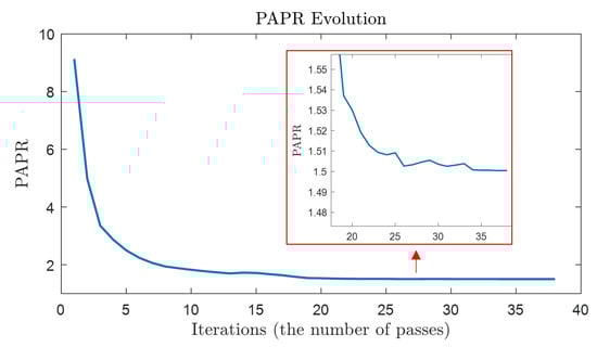
Figure 9.
PAPR evolution over iterations.
The final sequence shown in Figure 10 has the same power spectrum as of the initial sequence (see Figure 7a) and thus its ACF (see Figure 7b) has been preserved. It should be noted that when the waveform is up-sampled for the generation of an IF signal, the PAPR may increase by 2–3 dB [25] in general. Thus, it is suggested that either an a priori margin be considered for the system or the signal be up-sampled (extended in the frequency domain via zeros padding) to the rate before running the PAPR reduction algorithm.
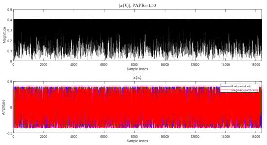
Figure 10.
The PAPR optimized COSPAR signal (PAPR = 1.5). The power spectrum and ACF of the signal omitted here are the same as in Figure 7b,c.
2.4. Step IV: Quadrature Vector Modulator and Upconversion
The complex baseband signal synthesized by the COSPAR method must be up-converted to the IF band in the final step such that the discrete samples of the synthetic waveform can be fed to DAC for transmission. Assuming an integer oversampling factor , we particularly append zeros to both sides of the COSPAR spectrum to extend its sample size to , where is the sample size of the complex baseband signal. This extension in the frequency domain is equivalent to SINC interpolation applied in the time domain. After that, we up-convert the interpolated complex signal to the IF band according to the following quadrature vector modulation procedure:
where is the center frequency of the IF band and is the real IF band signal.
Example 3
Using the COSPAR waveform synthesized in Step III (Example 2), we consider up-converting the baseband signal to the IF band (200 MHz–300 MHz) given the DAC sampling rate of 1200 MSPS. Thus, the oversampling factor is . Then, the sample size is extended in the frequency domain, and as such the new sample size becomes . Finally, the real signal is obtained by applying quadrature vector modulation with The power spectrum of the real COSPAR signal is shown in Figure 11.
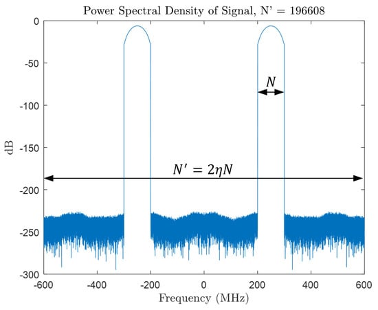
Figure 11.
Power spectrum of IF band COSPAR signal (200–300 MHz).
3. Range Resolution of COSPAR Signals
In general, the radar range resolution for radars using modulated signals with a bandwidth of is defined as , where is the speed of light. This is in fact the distance between the −3 dB points with respect to the peak response (mainlobe) in the ACF. In the COSPAR signal generation procedure, the desired level of correlation sidelobes and the parameters chosen to generate the Taylor window function modify the original slightly by a factor . Then, for a COSPAR signal with a bandwidth extend of , the approximation to the modified range resolution can be given as the following:
and the mainlobe broadening factor is determined by:
where and are given as in Equation (14) and Equation (15), respectively. Figure 12 shows the mainlobe modification factor for various lateral lobe parameters.
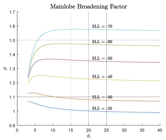
Figure 12.
Mainlobe broadening factor for various and values.
4. Orthogonality of COSPAR Signals
Each COSPAR synthesis leads to a distinct realization of a noise signal and thereby makes it possible to generate a set of mutually orthogonal noise waveforms. When transmitted successively, these orthogonal waveforms resolve range ambiguities in the radar while boosting the LPI property. Moreover, it permits a plurality of radars working in the same area and sharing the same spectrum. In Figure 13, the cross-correlation of two distinct COSPAR signals with the same energy and = 1.5 is shown. The cross-correlation level attains a mean level of .
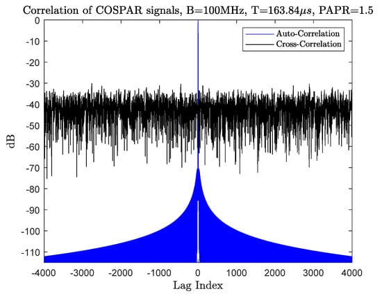
Figure 13.
Normalized cross-correlation and autocorrelation of two COSPAR realizations.
5. Ambiguity Function of COSPAR Signal
The Ambiguity Function (AF) of a signal is a representation of the signal’s matched filter response against various time delays and Doppler shifts and it can be used for the evaluation of signal resolution in Doppler and range space and for assessing waveforms’ Doppler tolerance [26,27]. The Ambiguity Function of a signal can be defined as:
where and are time delay and Doppler frequency, respectively.
A comparison of COSPAR and typical LFM (chirp) signal AFs is shown in Figure 14. In this respect, the LFM waveform is Doppler tolerant such that the matched filter still outputs a peak when the return signal incurs a Doppler frequency shift despite some offset in the target’s apparent range. This is called “range-Doppler coupling”, and to identify the true range, most often an up and down chirp pair is used to average the detection offset from opposite slopes of each chirp AF [28]. On the other hand, COSPAR represents a typical noise waveform with a thumbtack AF shape bearing high range and Doppler resolution. However, in this case, the Doppler shift will result in a reduction in processing gain, and as a result, target response SNR will decrease severely. Thus, noise waveforms are considered as Doppler sensitive. In noise radars, this problem is resolved by performing pulse compression with a bank of filters matched to a selection of desired Doppler frequencies or by the efficient range-filter bank method described in [29].
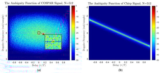
Figure 14.
(a) Ambiguity Function of COSPAR signal. (b) Ambiguity Function of LFM signal.
However, in a continuous wave noise radar, the waveform with appropriate integration time can still be Doppler tolerant for practical applications. For example, in the X-band (e.g., 9.3–9.4 GHz) marine radar case, the typical vessel velocity ranges between 0 and 30 m/s (0–60 kts), leading to a Doppler frequency shift at the maximum. If we use a noise signal with a duration of 164.83 such as the COSPAR signal synthesized in Example 3, then we would still obtain a target response out of the matched filter, as shown in Figure 15a. No range offset occurs and the SNR loss (~0.05 dB) in peak response due to Doppler shift is negligible (see Figure 15b) for COSPAR signals.
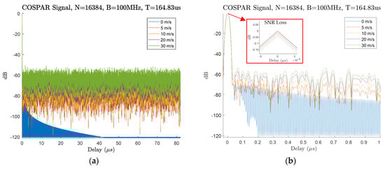
Figure 15.
(a) Normalized correlation functions under varying Doppler velocities for 0 m/s, 5 m/s, 10 m/s, 20 m/s, 30 m/s. (b) Correlation sidelobes adjacent to mainlobe and SNR loss due to Doppler mismatch.
6. LPI Property of COSPAR Signal: Spectral and Time–Frequency Analysis
As for the temporal analysis, the noise-like properties of COSPAR signals are discussed in previous sections. From the spectral point of view, the COSPAR signal attains a deterministic spectral shape (e.g., Figure 7b) prescribed by the Taylor window function during its synthesis, which could be considered as a weakness in terms of Electronic Protection at first glance. However, unless the exact duration and bandwidth of the signal are known a priori, estimating the spectrum of the continuous emission COSPAR signal from the arbitrary capture of its transmissions is no easier than any other conventional LPI waveforms. Owing to the Taylor window function, there are no spectral discontinuities and its favorable smooth roll-off at band edges makes it a good candidate for LPI operation. Moreover, its strength lies in its time–frequency representation discussed herein.
Modern ESM systems are capable of generating time–frequency analysis maps apart from traditional spectral analysis methods [30]. In this way, these ESM systems are able to intercept the widely used LFM and its variant NLFM signals of the so-called LPI radars. Some methods used in time–frequency domain signal analysis are based on:
- Short Time Fourier Transform (STFT) [31].
- Wigner–Ville Distribution (WVD) [32].
- Choi–Williams Distribution (CWD) [33].
Time–frequency plots provide a better insight into the signal than traditional methods. Thus, to evaluate and compare the time–frequency distribution of traditional LFM and COSPAR waveforms, the STFT and Wigner–Ville Distribution of these signals are shown in Figure 16a–d. Our first observation is that the energy of the COSPAR signal is well spread over the whole time–frequency plane, which makes signal analysis by the electronic reconnaissance system impractical. Therefore, it is believed that extracting signal features from the COSPAR signal analysis is a challenging task for ESM receivers. Then the question is “How can we say that the signal appears as noise and is suitable for LPI operation?”
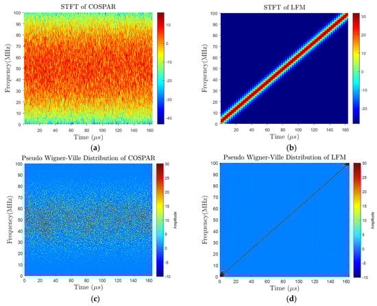
Figure 16.
(a) STFT of COSPAR signal. (b) STFT of LFM signal. (c) Pseudo Wigner–Ville Distribution of COSPAR signal. (d) Pseudo Wigner–Ville Distribution of LFM signal.
In order to quantify the LPI properties, we refer to the Spectral Kurtosis (SK) measure in this work. Spectral Kurtosis is a statistical tool that can reveal non-stationary and non-Gaussian distribution in the frequency domain for each frequency component. A small value of Spectral Kurtosis for a frequency bin indicates stationary Gaussian noise is present, whereas a high positive value pinpoints the existence of a transient or structured signal at the corresponding frequency [34,35]. This makes Spectral Kurtosis a useful and powerful tool for quantifying the LPI properties of waveforms for noise radar.
The Spectral Kurtosis of a signal can be computed based on its spectrogram, which is obtained by the STFT (Short Time Fourier Transform) :
where is the window function used in STFT. Then, SK is defined by:
where ⟨ ⟩ is the time-average operator.
As shown in Figure 17, the distribution of frequency bins over time for the COSPAR signal tends to have a normal distribution, giving a Spectral Kurtosis value of nearly zero, indicating such a noise-like distribution (normal distribution) for all frequencies. On the other hand, the LFM signal possesses a high value of Spectral Kurtosis over the entire frequency band, which means the signal has a structured time–frequency support. Considering an ESM receiver, the COSPAR signal can be buried well under the ESM receiver’s internal thermal noise, making it difficult for the ESM system to distinguish due to the signal’s noise-like behavior.
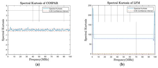
Figure 17.
(a) Spectral Kurtosis of COSPAR signal. (b) Spectral Kurtosis of LFM signal.
7. Field Experiments
In January 2021, marine trials were conducted in the shore-based test site of Turkish Naval Research Center Command (TNRCC) using the noise radar demonstrator developed by TNRCC. The demonstrator system conforms to the architecture shown in Figure 1. The demonstrator was set to work in X-band during trials and raw data from marine targets of opportunity were collected for offline analysis. A radar scan view of the scene generated using COSPAR recordings shows various ship targets at sea and land structures around the test site up to 8 km in Figure 18.
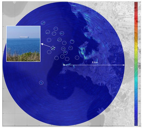
Figure 18.
A surveillance scan view obtained using COSPAR signal. Ship targets are encircled in white. The large ship target marked with dashed white circle is used for range profile analysis.
During these trials, the COSPAR signal (having a bandwidth MHz and duration ) generated in Example 3 was used and outcomes are compared with results obtained using a 100 MHz Gaussian noise waveform with the same radar settings. In order to compare the COSPAR sidelobe performance against a Gaussian noise waveform, we recorded the raw data while the demonstrator system was kept staring at the ship target at a distance of about 2400 m, which is marked with a dashed white circle in Figure 18. The correlation spikes belonging to the ship are apparent in both of the range profiles seen in Figure 19. Observing the range profile, we can make this simple observation: the strongest echo from the ship is about 8 dB above the leakage level (0 dB) and the SNR for the target is equal to ~48 dB for the COSPAR waveform, whereas it is ~38 dB for the Gaussian noise case. Considering the strongest echo from the ship, the matched filter dynamic range floor is dominated by sidelobes of the target response, not the leakage. For both waveforms, the sidelobes are not at the expected level (−60 dB for COSPAR and −42 dB for Gaussian noise) due to ground clutter near the radar and the quantization noise of the digital converters. However, it is clearly seen that the dynamic range can be improved with the usage of tailored waveforms such as COSPAR signals. In this respect, we have shown the usefulness of the proposed COSPAR waveform for a typical noise radar application.
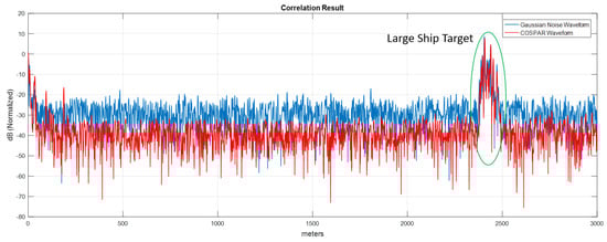
Figure 19.
Comparison of range profiles of the ship target for Gaussian noise and COSPAR waveform. COSPAR provides more room for better target SNR by having lower sidelobes than Gaussian noise.
8. Conclusions
In this paper, the fundamental noise radar architecture and its correlation processing have been reviewed along with important performance aspects related to waveform choice for noise radars, and a novel noise waveform synthesis method (called “Combined Spectral Shaping and Peak-to-Average Power Reduction, COSPAR”) including a cyclic PAPR reduction algorithm has been presented. Its main advantages are its low computational complexity and its simplicity for hardware implementation. The method allows parametric spectral shape synthesis such that designers can specify the Taylor window properties for spectral shape synthesis and adjust the corresponding ACF near-in sidelobes and peak sidelobe level accordingly.
The COSPAR waveforms are a special case within the general class of noise radar waveforms that while bearing a deterministic power spectral shape, every realization generates a different time domain signal, each having a distinct time–frequency distribution that makes them amenable for enhanced LPI operation. In this respect, these waveforms are non-repetitive and thus cannot be easily predicted or intercepted by ESM receivers.
COSPAR waveforms enjoy many valuable attributes, some of which can be summarized as follows:
- (i)
- COSPAR waveforms are noise-like. Although they possess a deterministic spectral shape, it has been shown that the signal energy is well distributed over their time–frequency plane. Signals which have structured time–frequency support or signals which concentrate energy within a certain band are easily intercepted at a great distance by the ESM receiver. In this respect, COSPAR waveforms possess good LPI attributes.
- (ii)
- Signal energy does not vary radically from pulse to pulse due to its pre-specified and fixed power spectrum. Therefore, target SNR fluctuation (due to inconstant transmit signal energy from pulse-to-pulse) is eliminated.
- (iii)
- Matched filter outputs are not affected by random range sidelobe modulation due to its pre-defined autocorrelation shape, and standard pulse compression radar signal processing techniques can be applied.
- (iv)
- Its Ambiguity Function tends to be thumbtack shape, which resolves range and Doppler ambiguities.
Moreover, the possibility to shape the underlying autocorrelation function by the parametric spectral shape synthesis (i.e., Taylor window) makes this type of waveform potentially useful for many sensing applications such as automotive radar, marine navigation radar, surveillance radar, SAR imaging and MIMO radar. Consequently, COSPAR signals represent a form of waveform diversity for noise radars offering degrees of freedom to control sidelobe level and crest factor that can be readily explored in many sensing measurements.
Author Contributions
Conceptualization, K.S.; methodology, K.S.; software, K.S.; validation, K.S., G.G., and G.P.; formal analysis, G.G. and G.P.; investigation, G.G. and G.P.; writing—original draft preparation, K.S.; writing—review and editing, K.S., G.G. and G.P. All authors have read and agreed to the published version of the manuscript.
Funding
This research received no external funding.
Institutional Review Board Statement
Not Applicable.
Informed Consent Statement
Not Applicable.
Data Availability Statement
Not Applicable.
Acknowledgments
We thank the Italian University Consortium for Telecommunications—CNIT for its contribution to the publication of this work.
Conflicts of Interest
The authors declare no conflict of interest.
Abbreviations
The following abbreviations are used in this manuscript:
| ACF | Auto Correlation Function |
| CA | Cyclic Algorithm |
| COSPAR | Combined Spectral Shape and Peak-to-Average-Power Ratio Reduction |
| CW | Continuous Wave |
| CWD | Choi–Williams Distribution |
| DSP | Digital Signal Processor |
| DFT/IDFT | Discrete Fourier Transform/Inverse DFT |
| EA | Electronic Attack |
| EP | Electronic Protection |
| ESM | Electronic Support Measures |
| FFT/IFFT | Fast Fourier Transform/Inverse FFT |
| FMCW | Frequency Modulated Continuous Wave |
| FPGA | Field Processing Gate Array |
| LFM | Linear Frequency Modulation |
| MF | Matched Filter |
| NLFM | Nonlinear Frequency Modulation |
| PAPR | Peak-to-Average Power Ratio |
| PSD | Power Spectral Density |
| PSL | Peak Sidelobe Level |
| PR | Phase Retrieval |
| RCS | Radar Cross Section |
| SNR | Signal-to-Noise Ratio |
| STFT | Short Time Fourier Transform |
| WVD | Wigner–Ville Distribution |
References
- Galati, G.; Pavan, G.; De Palo, G.F. Compatibility problems related with pulse-compression, solid-state marine radars. IET Radar Sonar Navig. 2016, 10, 791–797. [Google Scholar] [CrossRef]
- Kulpa, K. Signal Processing in Noise Waveform Radar; Artech House: Norwood, MA, USA, 2013. [Google Scholar]
- Popov, A.S.; Rybkin, P.N.; Vasil’ev, V.F. The report of experiments on electrical wireless signalization performed by a mine detachment during the campaign of 1897. In Collection of Documents and Materials 50 Years of Radio; Invention of Radio by A.S. Popov; Berg, A.I., Ed.; The Academy of Sciences of the U.S.S.R.: Moscow, Russia, 1945. (In Russian) [Google Scholar]
- Hülsmeyer, C. Verfahren, um entfernte metallische gegenstände mittels elektrischer wellen einem beobachter zu melden. German Patent 165,546, 30 April 1904. [Google Scholar]
- Hülsmeyer, C. The Telemobiloscope. Electr. Mag. 1904, 2, 388. [Google Scholar]
- Bourret, R. A proposed technique for the improvement of range determination with noise radar. IRE Proc. 1957, 45, 1744. [Google Scholar]
- Hourton, B.M. Noise-modulated distance measuring system. IRE Proc. 1959, 49, 821–828. [Google Scholar] [CrossRef]
- Savci, K. Noise Radar-Overview and Recent Developments. IEEE Aerosp. Electron. Syst. Mag. 2020, 35, 8–20. [Google Scholar] [CrossRef]
- Galati, G.; Pavan, G.; Savci, K.; Wasserzier, C. Noise Radar Technology: Waveforms Design and Field Trials. Sensors 2021, 21, 3216. [Google Scholar] [CrossRef]
- Pralon, L.; Beltrao, G.; Barreto, A.; Cosenza, B. On the Analysis of PM/FM Noise Radar Waveforms Considering Modulating Signals with Varied Stochastic Properties. Sensors 2021, 21, 1727. [Google Scholar] [CrossRef] [PubMed]
- Galati, G.; Pavan, G.; De Palo, F.; Stove, A.G. Potential applications of noise radar technology and related waveform diversity . In Proceedings of the 17th International Radar Symposium (IRS 2016), Krakow, Poland, 10–12 May 2016; pp. 1–5. [Google Scholar]
- Palo, F.; Galati, G.; Pavan, G.; Wasserzier, C.; Savci, K. Introduction to Noise Radar and Its Waveforms. Sensors 2020, 20, 5187. [Google Scholar] [CrossRef]
- Turin, G. An introduction to matched filters. IRE Trans. Inf. Theory 1960, 6, 311–329. [Google Scholar] [CrossRef]
- He, H.; Li, J.; Stoica, P. Waveform Design for Active Sensing Systems; Cambridge University Press: Cambridge, UK, 2012. [Google Scholar]
- Savci, K.; Erdogan, A.Y. Digital Correlator: A Scalable and Efficient FPGA Implementation for Radar Receivers. In Proceedings of the Signal Processing Symposium (SPSympo 2019), Krakow, Poland, 17–19 September 2019; pp. 207–211. [Google Scholar]
- Prabhu, K.M. Window Functions and Their Applications in Signal Processing, 1st ed.; CRC Press: Boca Raton, FL, USA, 2017. [Google Scholar]
- Doerry, A. ; Catalog of Window Taper Functions for Sidelobe Control; Sandia National Laboratories: Albuquerque, MN, USA, 2017. [Google Scholar]
- Taylor, T.T. Design of line-source antennas for narrow beamwidth and low side lobes. Trans. IRE Prof. Group Antennas Propag. 1955, 3, 16–28. [Google Scholar] [CrossRef]
- Carrara, W.G.; Goodman, R.S.; Majewsli, R.M. Spotlight Synthetic Aperture Radar Signal Processing Algorithms; Artech House: Norwood, MA, USA, 1995; pp. 512–513. [Google Scholar]
- Ann, P.P.; Jose, R. Comparison of PAPR reduction techniques in OFDM systems. In Proceedings of the International Conference on Communication and Electronics Systems (ICCES), Coimbatore, India, 21–22 October 2016; pp. 1–5. [Google Scholar]
- Han, S.H.; Lee, J.H. An overview of peak-to-average power ratio reduction techniques for multicarrier transmission. IEEE Wirel. Commun. 2005, 12, 56–65. [Google Scholar] [CrossRef]
- Tropp, J.A.; Dhillon, I.S.; Heath, R.W.; Strohmer, T. Designing structured tight frames via an alternating projection method. IEEE Trans. Inf. Theory 2005, 51, 188–209. [Google Scholar] [CrossRef]
- Taylor, L. The phase retrieval problem. IEEE Trans. Antennas Propag. 1981, 29, 386–391. [Google Scholar] [CrossRef]
- Gerchberg, R.W.; Saxton, W.O. A practical algorithm for the determination of the phase from image and diffraction plane pictures. Optik 1972, 35, 237. [Google Scholar]
- Han, S.H.; Lee, J.H. PAPR reduction of OFDM signals using a reduced complexity PTS technique. IEEE Signal Process. Lett. 2004, 11, 887–890. [Google Scholar] [CrossRef]
- Woodward, P.M. Probability and Information Theory with Applications to Radar; McGraw-Hill: New York, NY, USA, 1953. [Google Scholar]
- Levanon, N.; Mozeson, E. Radar Signals; Wiley: Hoboken, NJ, USA, 2004. [Google Scholar]
- Rihaczek, A.W. Principles of High Resolution Radar; Artech House: Norwood, MA, USA, 1996. [Google Scholar]
- Wasserzier, C.; Galati, G. On the efficient computation of range and Doppler data in noise radar. Int. J. Microw. Wirel. Technol. 2019, 11, 584–592. [Google Scholar] [CrossRef]
- Pace, P. Detecting and Classifying Low Probability of Intercept Radar, 2nd Ed. ed; Artech House: Norwood, MA, USA, 2009. [Google Scholar]
- Cohen, L. Time-Frequency Analysis; Prentice Hall: Hoboken, NJ, USA, 1995. [Google Scholar]
- Ville, J. Theorie et applications de la notion de signal analytique. Cables Transm. 1948, 2, 61–74. [Google Scholar]
- Choi, H.I.; Williams, W.J. Williams Improved time-frequency representation of multicomponent signals using exponential kernels. IEEE Trans. Acoust. Speech Signal Process. 1989, 37, 862–871. [Google Scholar] [CrossRef]
- Antoni, J. The Spectral Kurtosis: A Useful Tool for Characterising Non-Stationary Signals. Mech. Syst. Signal Process. 2006, 20, 282–307. [Google Scholar] [CrossRef]
- Antoni, J.; Randall, R.B. The Spectral Kurtosis: Application to the Vibratory Surveillance and Diagnostics of Rotating Machines. Mech. Syst. Signal Process. 2006, 20, 308–331. [Google Scholar] [CrossRef]


Publisher’s Note: MDPI stays neutral with regard to jurisdictional claims in published maps and institutional affiliations. |
© 2021 by the authors. Licensee MDPI, Basel, Switzerland. This article is an open access article distributed under the terms and conditions of the Creative Commons Attribution (CC BY) license (https://creativecommons.org/licenses/by/4.0/).