Coarse-to-Fine Loosely-Coupled LiDAR-Inertial Odometry for Urban Positioning and Mapping

Abstract

Accurate positioning and mapping are significant for autonomous systems with navigation requirements. In this paper, a coarse-to-fine loosely-coupled (LC) LiDAR-inertial odometry (LC-LIO) that could explore the complementariness of LiDAR and inertial measurement unit (IMU) was proposed for the real-time and accurate pose estimation of a ground vehicle in urban environments. Different from the existing tightly-coupled (TC) LiDAR-inertial fusion schemes which directly use all the considered ranges and inertial measurements to optimize the vehicle pose, the method proposed in this paper performs loosely-couped integrated optimization with the high-frequency motion prediction, which was produced by IMU integration based on optimized results, employed as the initial guess of LiDAR odometry to approach the optimality of LiDAR scan-to-map registration. As one of the prominent contributions, thorough studies were conducted on the performance upper bound of the TC LiDAR-inertial fusion schemes and LC ones, respectively. Furthermore, the experimental verification was performed on the proposition that the proposed pipeline can fully relax the potential of the LiDAR measurements (centimeter-level ranging accuracy) in a coarse-to-fine way without being disturbed by the unexpected IMU bias. Moreover, an adaptive covariance estimation method employed during LC optimization was proposed to explain the uncertainty of LiDAR scan-to-map registration in dynamic scenarios. Furthermore, the effectiveness of the proposed system was validated on challenging real-world datasets. Meanwhile, the process that the proposed pipelines realized the coarse-to-fine LiDAR scan-to-map registration was presented in detail. Comparing with the existing state-of-the-art TC-LIO, the focus of this study would be placed on that the proposed LC-LIO work could achieve similar or better accuracy with a reduced computational expense.

1. Introduction

Positioning and mapping are undoubtedly essential modules for autonomous tasks, such as autonomous driving and robotic service, in unknown or partially known environments. It is well known that the Global Navigation Satellite System (GNSS) could provide satisfactory performance in open-sky areas. However, due to the reflection caused by static skyscrapers and dynamic tall objects such as double-decker buses, reflected signals from the same satellite could be received and the notorious non-light-of-sight (NLOS) receptions occur [1], which is the major difficulty significantly degrading the positioning accuracy and preventing GNSS from utilization in intelligent transportation systems under urban canyons [2]. The local perception sensor, Laser Detection and Ranging (LiDAR) has attracted great attention owing to its high precision, reliability, long perception distance and insensitivity to illumination. The major principle of LiDAR-based positioning and mapping is to track the motions obtained by registrations between consecutive frames of point clouds [3]. However, the LiDAR standalone-based odometry is sensitive to motion distortions especially in high-speed motion under highly urbanized environments with numerous dynamic objects [4]. As per a study [5], for a Velodyne HDL-64E swiping at 10 Hz, a linear motion at 50 km/h could generate a gap of 1.38m between the beginning and the end of a scan. A rotational motion at 25 degree/s could generate a gap of 2.19 m at 50 m away from the LiDAR. Moreover, the point cloud registration of LiDAR odometry relies on an accurate initial guess which is hard to obtain without the assistance of other sensors [6]. Considering the complementariness of the LiDAR and the inertial measurement unit (IMU), the researchers proposed diverse LiDAR-inertial odometry (LIO) pipelines.

Odometry schemes based on LiDAR-inertial fusion are extensively investigated. One category is tightly-coupled (TC) fusion, which allows the direct fusion of measurements from sensor outputs and has recently gained widespread utilization. TC methods are based on the filter [7] or the factor graph optimization [8], both of which have been well studied. LINS [9], in which an iterated error state Kalman filter with robocentric formulation is employed, provides real-time ego-motion estimation. However, it has been shown in our recent work [10] that the factor graph optimization-based sensor fusion can better employ the correlation between consecutive epochs of measurements simultaneously, compared with the extended Kalman filter (EKF)-based estimator. Instead of adopting the filtering-based sensor fusion, the Lio-mapping framework [11] was proposed, optimizing measurements from LiDAR (point-to-map association) and IMU pre-integration in a sliding window via a factor graph. However, the accuracy highly depends on the quality of the IMU on the ground that the IMU measurements are directly fused with the point-to-map registration to generate the final state of the vehicle. Furthermore, such TC integration induces a significantly high computation load thus cannot guarantee real-time performance. The major computation load is caused by the point-to-map association, which is similar to the visual reprojection [12], of each LiDAR frame during sliding window optimization. In order to solve this problem, the LIO-SAM [13] is proposed for the implementation of the keyframe-based tightly-coupled LiDAR-inertial odometry (TC-LIO) based on factor graph optimization via incremental smoothing and mapping [14]. Local scan-to-map registration [15] and keyframe selection are beneficial to real-time performance. Recently, there is an inspiring work [16], the LiLi-OM, which presents a TC-LIO and mapping system. Interestingly, two independent factor graphs are maintained by LiLi-OM. One larger factor graph is in charge of integrating IMU pre-integration with LiDAR feature association of selected keyframes and performing sliding window-based optimization; while the other smaller factor graph within the sliding window is invoked to obtain poses of frames that are not selected as keyframes. The LiLi-OM is evaluated on multiple challenging datasets (e.g., the UrbanLoco dataset [4] and the KITTI dataset [17]) with the results showing that the LiLi-OM significantly outperforms the LIO-SAM and the Lio-mapping. In other words, the LiLi-OM is currently the most state-of-the-art TC-LIO scheme. Nevertheless, it is still inevitable that the computation load is high and the performance is limited by IMU during TC integrations.

The other category of LiDAR-inertial fusion is loosely-coupled (LC) fusion, which allows the fusion of respective motion estimations from LiDAR odometry and IMU integrations. In LOAM [3] and LeGO-LOAM [18], which are typical LiDAR odometry algorithms, IMU is employed to provide high-frequency motion prediction for LiDAR odometry. Meanwhile, the motion distortion is partially solved. However, the bias of the IMU is not corrected due to the assumption [3,18] that the impact of the IMU bias in a short period can be ignored. Furthermore, an LC fusion of LiDAR and IMU [19] is achieved through varieties of Kalman filters, which allows the fusion of LiDAR positioning results with rotational velocity from IMU with the aim of testing on vehicles equipped with low-mounted multiple LiDARs. Similarly, a 2D indoor navigation system [20] is developed through EKF fusing standalone positioning results from LiDAR and IMU separately. However, the EKF can only execute linear approximation once at a fixed operating point [21]. More importantly, EKF is subject to the first-order Markov hypothesis, under which the historical information cannot be fully utilized by the current state [21]. Therefore, the EKF-based LC methods are considered to be computationally efficient but sensitive to gross outlier measurements [22]. Fortunately, the factor graph-based LC LiDAR-inertial positioning and mapping system retains the high precision of iterative optimization and low computational complexity of decoupled formulation. Furthermore, the computational efficiency can be enhanced on account of sliding window-based optimization. As mentioned above, correlation between consecutive frames of measurements can be employed within an optimization window, which, therefore, also conduces to the accuracy. Nevertheless, for pure loosely-couped LiDAR/inertial odometry (LC-LIO), the problem that the performance is limited by the quality of IMU still exists.

In this paper, a coarse-to-fine LC-LIO for urban positioning and mapping was proposed to deal with the aforementioned problems. On the one hand, the window-based factor graph optimization (coarse process) is adopted to estimate the bias of the IMU by integrating the IMU pre-integration and the LiDAR scan-to-map registration. Therefore, the motion distortion can be mitigated by the high-frequency IMU integration based on the corrected IMU bias. Moreover, real-time performance is guaranteed thanks to the decoupled integration and window-based optimization. On the other hand, the refinement of LiDAR scan-to-map registration (fine process) is performed to estimate the pose of the vehicle based on the initial guess from the coarse process. Theoretically, the accuracy of the LiDAR ranging measurement is centimeter-level and a similar accuracy of motion estimation could be derived based on the LiDAR scan-to-map registration. However, in practice, only the locally optimal solution with larger error is usually obtained due to the fact that the LiDAR scan-to-map registration is mathematically a non-convex optimization. It is well-known that providing an accurate initial guess for the non-linear optimization could significantly contribute to removing the local minimum and converging to an ideal optimal solution. In light of this, the initial guess produced via high-frequency IMU integration based on the optimized state estimation from the coarse process could further relax the high accuracy of LiDAR ranging measurements, which would induce an accurate motion estimation. It can be considered that the contributions of this paper include three aspects:

• Development of a coarse-to-fine LC-LIO pipeline based on window optimization. Meanwhile, the adaptive covariance estimation of the LiDAR scan-to-map registration is proposed for further LiDAR/Inertial integration.
• Theoretical analysis of performance upper bound of LC and TC LiDAR-inertial fusion considering the error propagation from LiDAR and inertial measurements.
• Validation of the proposed method with challenging datasets collected in urban canyons of Hong Kong. The convergence results of both the LC-LIO and TC-LIO are presented to experimentally verify the theoretical analysis in the second aspect.

The remainder of this paper is arranged as follows. Firstly, the overall framework of the proposed system would be elucidated in Section 2. Furthermore, details of the LC optimization framework would be expounded in detail in Section 3, including the illustration of the proposed factor graph (Section 3.1), IMU measurement modeling (Section 3.2), LiDAR measurement modeling (Section 3.3) and adaptive information matrix description (Section 3.4). Moreover, the theoretical analysis of the upper bound of both LIOs would be described in Section 4. Furthermore, the implementation and experimental results would be interpreted in Section 5. Finally, a conclusion of this study would be presented in Section 6.

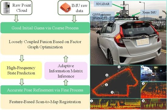
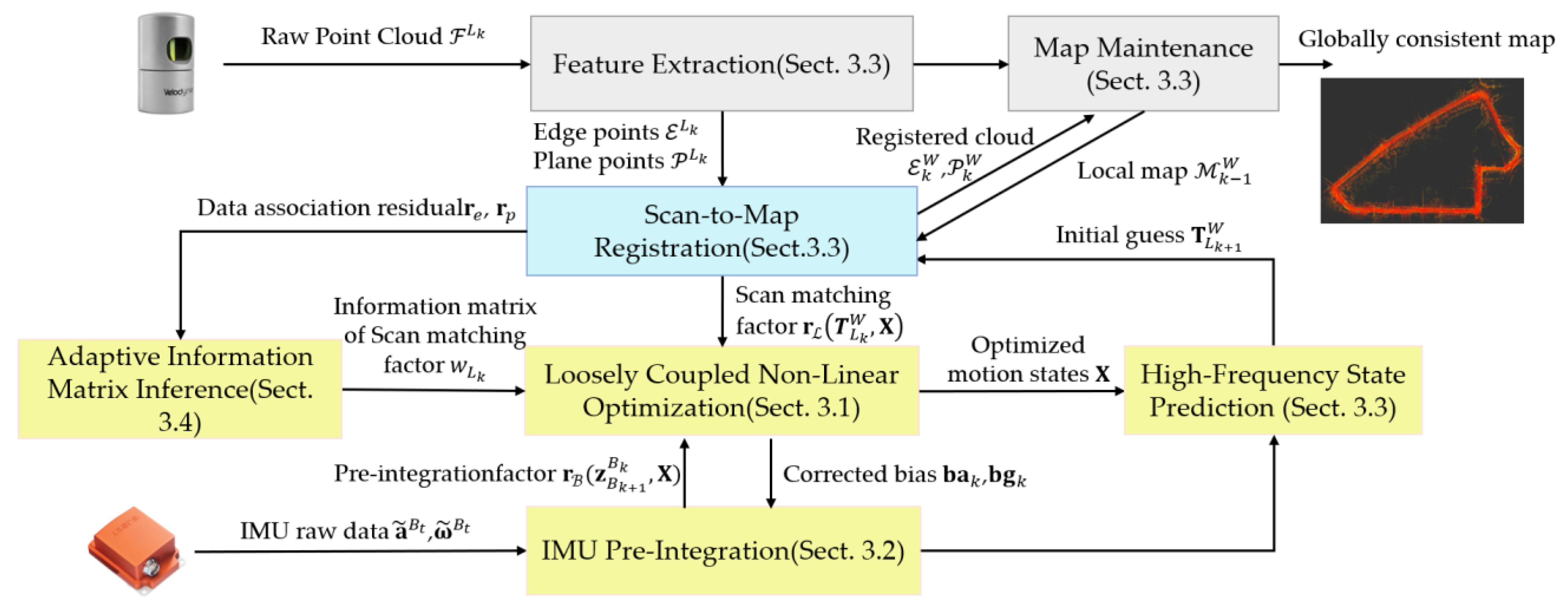
2. Overview of the Proposed LC-LIO

The structure of the proposed LIO is shown in Figure 1, which is a coarse-to-fine LC integration system based on factor graph optimization. The yellow and blue represent the coarse and fine processes, respectively. The inputs of the system include the raw 3D point clouds from the 3D LiDAR and gyroscope and accelerometer readings from IMU. The output is the six-degree-of-freedom pose of LiDAR and a globally consistent map. As per the raw point clouds from LiDAR, the feature points on sharp edges and planar surface patches are extracted first [3]. IMU measurements between the current and the last LiDAR frames are pre-integrated.

In terms of the coarse process, pre-integration results and the scan-to-map registration results will construct the pre-integration factor and the scan matching factor, respectively, during the current LC non-linear optimization. Residuals of scan-to-map registration will be converted to an information matrix of the scan matching factor by an exponential function. Based on the optimized states and IMU measurements, high-frequency motion state prediction is performed to provide an initial guess for the scan-to-map registration of the next LiDAR frame.

In terms of the fine process, a scan-to-map registration, employing the initial guess generated by the last LC optimization, is performed to achieve a fine estimation of the pose of LiDAR. A globally consistent map is also updated by registering the new coming point cloud to the map. The initial guess from the coarse process can exert significant impacts on the avoidance of falling into local optima and the removal of motion distortion of the point cloud. The details about the proposed method would be presented in the following sections.

Matrices are denoted as upper-case and bold letters. Vectors are denoted as lowercase with bold letters. Variable scalars are denoted as lower-case and italic letters. Constant scalars are denoted as lowercase letters. To clarify the proposed pipeline, the notations and frames used in the whole paper are defined as follows.

• The LiDAR body frame is represented as ${\{·\}}^L$, which is fixed at the center of the LiDAR sensor.
• The IMU body frame is represented as ${\{·\}}^{B }$, which is fixed at the center of the IMU sensor.
• The world frame is represented as ${\{·\}}^{W }$, which is originated at the initial position of the vehicle. It is assumed to coincide with the initial LiDAR frame.

The $k$-th frame of LiDAR point cloud is represented as ${ℱ}^{L_k}$. A frame is generated when LiDAR completes one-time scan coverage. The coordinate of a point $i$, $i\in {ℱ}^{L_k}$, under the $L_k$ coordinate is represented as $f_i^{L_k}$. The transformation matrix of the $k$-th frame of LiDAR point cloud under the world frame is represented as $T_{L_k}^W\in \mathrm{Special} \mathrm{Euclidean} \mathrm{Group} \left(SE\left(3\right)\right)$ [23]:

$$T_{L_k}^W=\left[\begin{array}{cc}{R}_{L_k}^W& p_{L_k}^W\\ 0& 1\end{array}\right],$$

(1)

where $p_{L_k}^W\in R^3$ stands for the translation, and $R_{L_k}^W\in \mathrm{Special} \mathrm{Orthogonal} \mathrm{Group}\left(3\right)\left(SO\left(3\right)\right)$ [24] stands for the rotation matrix. $SO\left(3\right)$ and $SE\left(3\right)$ are both Lie group [23]. In $SO\left(3\right)$ each element is an orthogonal matrix with the determinant 1 representing the rotation for 3D space. In $SE\left(3\right)$ each element consists of a rotation matrix and a translation vector representing the rigid motion for 3D space.

The $k$-th state of the IMU under the world frame, namely the state of the IMU at the time when the $k$-th frame of LiDAR point cloud is captured, can be expressed as:

$$x_k=\left[p_{B_k}^W,v_{B_k}^W,q_{B_k}^W,b{a}_k,b{g}_k\right],$$

(2)

where $x_k$ consists of the position $p_{B_k}^W$, velocity $v_{B_k}^W$, rotation $q_{B_k}^W$ in quaternion form, accelerometer bias $b{a}_k$ and gyroscope bias $b{g}_k$. Among them, the $k$-th transformation matrix of IMU can be represented as $T_{B_k}^W\in SE\left(3\right)$ [23]:

$$T_{B_k}^W=\left[\begin{array}{cc}{R}_{B_k}^W& p_{B_k}^W\\ 0& 1\end{array}\right],$$

(3)

where $R_{B_k}^W\in SO\left(3\right)$ represents the rotation matrix corresponding to $q_{B_k}^W$.

The extrinsic transformation matrix from the IMU body frame to the LiDAR body frame can be represented as $T_B^L$ which is calibrated offline. Therefore, the following transformations are satisfied:

$$T_{B_k}^W=T_B^L{T}_{B_k}^{B_0}$$

(4)

which transfers the pose under the initial IMU frame to that under the world frame, and it will be used during IMU measurements modeling.

$$T_{B_k}^W=T_{L_k}^W{T}_B^L$$

(5)

transfers the pose of LiDAR from the scan-to-map optimization to the pose of the corresponding IMU frame, which will be used during the loosely coupled optimization.

$$T_{L_k}^W=T_{B_k}^W{T}_B^L{}^{-1}$$

(6)

transfers the pose of IMU from the LC optimization to the pose of the corresponding LiDAR, which will be used during the high-frequency state prediction.

3. Coarse-to-Fine Loosely-Coupled LiDAR-Inertial Integration

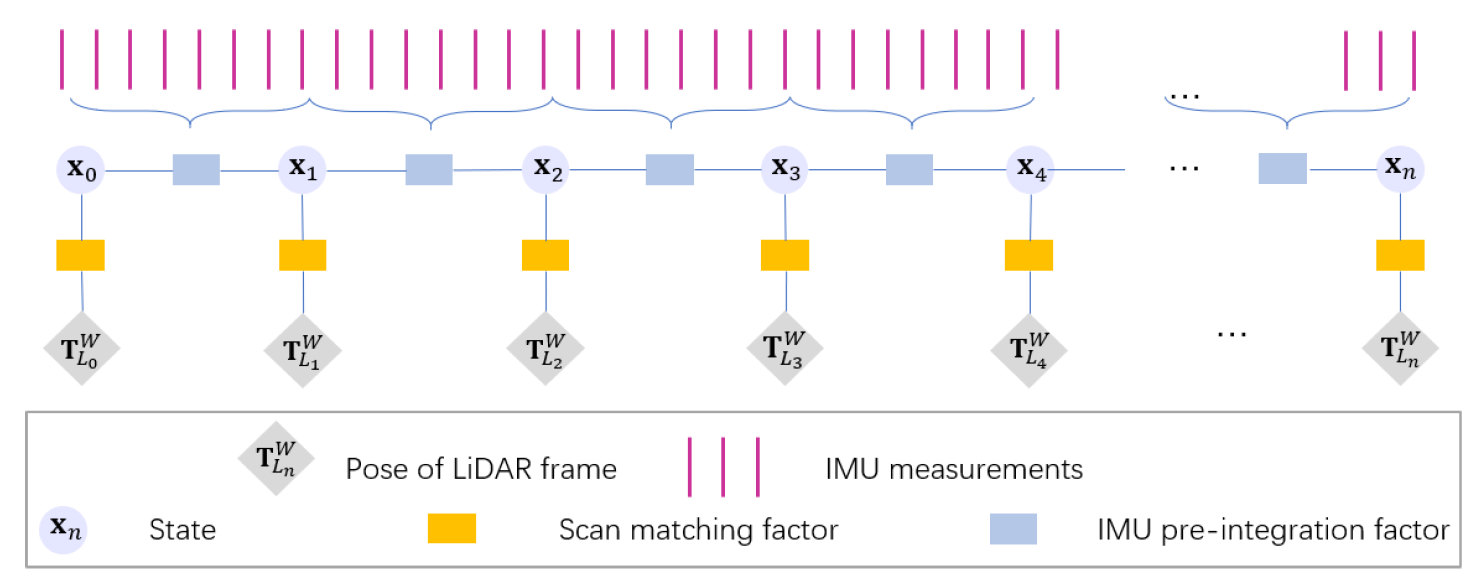
3.1. LC-LIO Factor Graph

The illustration of the proposed factor graph is presented in Figure 2 which contains one type of node and two types of edges. Every state of IMU, defined as (2), serves as one node in the graph. One kind of edge connects a single state $x_k$ with $k\in \left(0,n\right)$ and the pose of the corresponding LiDAR frame $T_{L_k}^W$. $T_{L_k}^W$ is generated by LiDAR scan-to-map registration. It can be regarded as a measurement in a joint optimization that could provide absolute constraints for the nodes to be optimized. IMU pre-integration results constrain the relative pose from one node to another, which is the other kind of edge.

LC-LIO estimates states of the IMU within a large window. As shown in Figure 2, the factor graph is quite sparse. There are only two or three constraints for one state. Thus, to achieve adequate constraints for the accurate estimation and maintain the real-time performance simultaneously, we maintain a fixed slide window containing 50 states during factor graph optimization [25]. Since the computation complexity increases linearly with the number of IMU states, using such a large window can still guarantee real-time capability. As shown in Figure 3, when the number of states included in the window reaches the pre-determined size, we preserve the last state and take it as the first frame in the new window. Different from the tightly-coupled LiDAR/Inertial integration, the correlation between the historical frames and the new coming ones is weaker [16]. Therefore, it is reasonable to remove the historical states to guarantee real-time performance.

Factor graph optimization is typically derived as a nonlinear least-squares problem. Once the graph is established, it can be solved by finding a group of states that conform to all edges best [8]. After adding all the weighted squared residuals generated by two kinds of edges in a window, the following equations can be obtained,

$$X=\underset{X}{\min }\frac{1}{2}\left\{{{\displaystyle \sum }}_{k\in \left\{0,\cdots ,n\right\}}\rho ({\parallel r_{ℒ}\left(T_{L_k}^W,X\right)\parallel }_{C_{L_k}}^2)+{{\displaystyle \sum }}_{k\in \left\{0,\cdots ,n-1\right\}}\rho ({\parallel r_{ℬ}\left(z_{B_{k+1}}^{B_k},X\right)\parallel }_{C_{B_{k+1}}^{B_k}}^2)\right\},$$

(7)

$$X=\left\{x_0,x_1,\cdots ,x_n\right\},$$

(8)

where, $r_{ℒ}\left(T_{L_k}^W,X\right)$ represents the residuals produced by LiDAR scan-matching factor, $z_{B_{k+1}}^{B_k}$ and $r_{ℬ}\left(z_{B_{k+1}}^{B_k},X\right)$ represents the measurements and the residuals produced by the IMU pre-integration factor, respectively. $X$ represents the states to be estimated. $n$ represents the size of the optimization window. The Mahalanobis norm is ${\parallel r\parallel }_C^2=r^T{C}^{-1}r$, where $C$ represents the covariance matrix of $r$, and $C^{-1}$ represents the so-called information matrix. $\rho$ represents the robust kernel to decrease the influence of outliers. The Cauchy kernel [26] is selected and defined as follows:

$$\rho \left(s\right)=\frac{c^2}{2}\log \left(1+\frac{s}{c^2}\right),$$

(9)

where $c$ represents a constant parameter that is set to $1$ [27]. Ceres solver [28] is used to solve this nonlinear problem and the Levenberg-Marquardt (L-M) algorithm [29] is employed to iteratively minimize the cost function. The detailed definition of residual terms and the adaptive information matrix of the LiDAR scan-to-map registration residual in (7) would be presented in Section 3.2, Section 3.3 and Section 3.4, respectively.

3.2. IMU Measurement Modeling

In this section, the modeling of the IMU measurements with pre-integration would be presented. Even though the pre-integration is not a main contribution from this paper, it would be elucidated in this section for the theoretical analysis in Section 4. The IMU measurements are the rotation rate and the acceleration of the system given in the IMU body frame. It is corrupted with the additive noise and a slowly varying bias of acceleration and gyroscope [30]:

$${\tilde{a}}^B=R_W^B\left(a^W-g^W\right)+ba+n_a,$$

(10)

$${\tilde{\mathsf{\omega }}}^B={\mathsf{\omega }}^B+bg+n_g.$$

(11)

It is worth noting that the transformation between the initial IMU frame ${\{·\}}^{B_0}$ and the world frame is taken into account in (4). For simplicity, it would be omitted in the equations in this section. ${\tilde{a}}^B$ represents the raw IMU acceleration measurements in the IMU body frame, and $a^W$ represents the noise-free acceleration of the system in the world frame. $g^W$ represents the gravity in the world frame. $R_W^B\in S{O}_3$ represents the rotation matrix from the world frame to the IMU body frame. $ba$ represents slowly varying acceleration bias, whose derivative is of Gaussian distribution.$n_a~\mathcal{N}\left(0, {\mathsf{\sigma }}_a^2\right)$ represents the additive noise of the acceleration. ${\tilde{\mathsf{\omega }}}^B$ is the raw IMU gyroscope measurements in the IMU body frame, ${\mathsf{\omega }}^B$ represents the noise-free rotation rate of $B$ relative to $W$ expressed in coordinate $B$. $bg$ represents the bias of ${\mathsf{\omega }}^B$. It can also be assumed that its derivative subjects to Gaussian distribution. $n_g~\mathcal{N}\left(0, {\mathsf{\sigma }}_g^2\right)$ represents the additive noise of ${\mathsf{\omega }}^B$.

There are dozens of or even hundreds of IMU measurements acquired between two consecutive LiDAR frames. The pre-integration theory is employed to model such a large number of IMU measurements as a single relative motion constraint [30]. The bias during this process is assumed to remain constant. It is implemented in a local frame so that repeated integration can be avoided when the IMU states have changed [31]. Otherwise, it will be a heavy computational burden.

In practice, IMU measurements are discrete and are synchronized with the LiDAR frames by linear interpolation. Median integral is employed to derive the pre-integration results. $B_t$ and $B_{t+1}$ are assumed to be two consecutive time instants between $B_k$ and $B_{k+1}$, and $\delta t$ represents the time interval between $B_t$ and $B_{t+1}$. The angular velocity and the acceleration during $\delta t$ can be expressed as:

$$\mathsf{\omega }=\frac{1}{2}\left(\left({\tilde{\mathsf{\omega }}}^{B_t}-b{g}_k\right)+\left({\tilde{\mathsf{\omega }}}^{B_{t+1}}-b{g}_k\right)\right)$$

(12)

In addition:

$$a=\frac{1}{2}\left(q_{B_t}^{B_k}\left({\tilde{a}}^{B_t}-b{a}_k\right)+q_{B_{t+1}}^{B_k}\left({\tilde{a}}^{B_{t+1}}-b{a}_k\right)\right)$$

(13)

The pre-integration of rotation $q_{B_{k+1}}^{B_k}$, velocity ${\mathsf{\beta }}_{B_{k+1}}^{B_k}$ and the translation ${\mathsf{\alpha }}_{B_{k+1}}^{B_k}$ between $B_k$ and $B_{k+1}$ under the $B_k$ coordinate is recursively derived, respectively, according to the following equations:

$$q_{B_{t+1}}^{B_k}=q_{B_t}^{B_k}\otimes \left[\begin{array}{c}0\\ \frac{1}{2}\mathsf{\omega }\delta t\end{array}\right],$$

(14)

$${\mathsf{\alpha }}_{B_{t+1}}^{B_k}={\mathsf{\alpha }}_{B_t}^{B_k}+{\mathsf{\beta }}_{B_t}^{B_k}\delta t+\frac{1}{2}a\delta t^2,$$

(15)

$${\mathsf{\beta }}_{B_{t+1}}^{B_k}={\mathsf{\beta }}_{B_t}^{B_k}+a\delta t.$$

(16)

The derived compound measurements generated by pre-integration can be represented as:

$$z_{B_{k+1}}^{B_k}=\left\{{\mathsf{\alpha }}_{B_{k+1}}^{B_k},{\mathsf{\beta }}_{B_{k+1}}^{B_k},q_{B_{k+1}}^{B_k},b{a}_{k+1},b{g}_{k+1}\right\},$$

(17)

It acts as the measurements of relative motion between two IMU states to constrain them. The residual $r_{ℬ}\left(z_{B_{k+1}}^{B_k},X\right)$ can be defined as:

$$r_{ℬ}\left(z_{B_{k+1}}^{B_k},X\right)={\left[\begin{array}{c}\begin{array}{c}{r}_p\\ r_q\\ r_v\end{array}\\ r_{ba}\\ r_{bg}\end{array}\right]}_{15\times 1}=\left[\begin{array}{c}{q}_{B_k}^W{}^{-1}\left(p_{B_{k+1}}^W-p_{B_k}^W-v_{B_k}^W\Delta t-\frac{1}{2}{g}^W\mathsf{\Delta }{t}^2\right)-{\mathsf{\alpha }}_{B_{k+1}}^{B_k}\\ 2{\left[q_{B_{k+1}}^{B_k}{}^{-1}\otimes \left(q_{B_k}^W{}^{-1}\otimes q_{B_{k+1}}^W\right)\right]}_{xyz}\\ q_{B_k}^W{}^{-1}\left(v_{B_{k+1}}^W-v_{B_k}^W-g^W\mathsf{\Delta }t\right)-{\mathsf{\beta }}_{B_{t+1}}^{B_k}\\ b{a}_{k+1}-b{a}_k\\ b{g}_{k+1}-b{g}_k\end{array}\right],$$

(18)

where ${[·]}_{xyz}$ extracts the imaginary part of a quaternion. Bias may be minorly corrected after each window optimization. The details are shown in Appendix A.

3.3. LiDAR Scan Matching Modeling

LiDAR achieves the range measurements between the LiDAR itself and the surrounded objects. As there is abundant three-dimensional geometry information in a deep urban canyon that is mainly man-made such as buildings, road signs and overpasses, it is feasible to extract enough edge points and plane points from LiDAR point clouds without further consideration of point density [32] and distribution [33]. The feature extraction manner [3] is employed here, through which the smoothness of the neighborhood around the operating point $f_i^{L_k}$ can be calculated as:

$$c=\frac{1}{\left|S\right|·\parallel f_i^{L_k}\parallel }\parallel {{\displaystyle \sum }}_{j\in S,j\ne i}\left(f_i^{L_k}-f_j^{L_k}\right)\parallel ,$$

(19)

where $S$ represents a set of neighbor points of $f_i^{L_k}$, which are on the same scan ring of $f_i^{L_k}$. $c$ represents the smoothness of $S$, $\left|S\right|$ represents the total number of points in $S$ and $\parallel ·\parallel$ represents the $L_2$ norm. Points with lower smoothness are selected as plane feature points, while points with larger smoothness are selected as edge points. Please refer to reference [3] for more details.

The pose of ${ℱ}^{L_k}$, $T_{L_k}^W$, is calculated by registering ${ℱ}^{L_k}$ to a local map ${ℳ}_{k-1}^W$ with a specified size [3,34]. The local map comprises the registered feature points of LiDAR frames before ${ℱ}^{L_k}$ and is organized in a KD-tree for efficient search. It will slide towards the current frame if the frame approaches the map boundary [35]. The current frame will always be kept inside the local map. Consequently, a significant number of point candidates are guaranteed for registration. If ${ℰ}^{L_k}$ and ${𝒫}^{L_k}$ are taken as the set of edge points and plane points of ${ℱ}^{L_k}$, respectively, the coordinates of points in these two sets will be under the ${ℱ}^{L_k}$ frame. If ${ℰ}^W$ and ${𝒫}^W$ are taken as the set of edge points and plane points of the local map, respectively, the coordinates of points will be under the world frame. During registration, for the $i$-th point $f_{e,i}^{L_k}\in {ℰ}^{L_k}$ and $f_{p,i}^{L_k}\in {𝒫}^{L_k}$, $T_{L_k}^W$ is employed to project them onto the local map as:

$$f_{(·),i}^W=T_{L_k}^W{f}_{(·),i}^{L_k},$$

(20)

where $(·)$ represents $e$ or $p$.

The initial guess of $T_{L_k}^W$ can be obtained by:

$$T_{L_k}^W=T_{L_{k-1}}^W\ast T_B^L\ast T_{B_k}^{B_{k-1}}\ast T_B^L{}^{-1},$$

(21)

where, $T_{L_{k-1}}^W$ represents the pose of the last LiDAR frame from LC optimization as per Equation (6). $T_{B_k}^{B_{k-1}}$ represents the motion increment between the last LiDAR frame and the current one, and it can be obtained from IMU measurement integrations as per Equations (12)~(16). The initial guess benefits from the accuracy of LC integration and high-frequency of IMU, and thus can improve the robustness of scan-to-map registration, especially in the degenerate case.

The final result of $T_{L_k}^W$ can be obtained through the iterative matching of these two categories of points, when $T_{L_k}^W$ is iteratively optimized until it converges, or the maximal number of iterations is finished. The objective of the feature matching is to minimize the point-to-line residuals from edge points and the point-to-plane residuals from plane points.

For an edge point $f_{e,i}^W$, there are 5 nearest edge points around it in ${ℰ}^W$ on the local map. Subsequently, eigendecomposition is performed on the covariance matrix of those five points. If the maximum eigenvalue is significantly larger than the other two, it is expectable for the five points to be on the same line of $f_{e,i}^W$. The line passes the geometric center of the five points $f_{c,ei}^W$ and its direction vector $\overrightarrow{n}$ is the eigenvector corresponding to the maximum eigenvalue. As shown in Figure 4a, the residual is formulated as the distance between $f_{e,i}^W$ and the simulated line:

$$r_{e,i}\left(f_{e,i}^{L_k},T_{L_k}^W\right)=d_{e,i}=\frac{\parallel \left(f_{e,i}^W-f_{e,1}^W\right)\times \left(f_{e,i}^W-f_{e,2}^W\right)\parallel }{\parallel f_{e,1}^W-f_{e,2}^W\parallel },$$

(22)

where, $f_{e,1}^W$ and $f_{e,2}^W$ are two points on the simulated line distributed on either side of $f_{c,ei}^W$ [16]. For a plane point $f_{p,i}^W$, there are also 5 nearest plane points around it on the map, which can be represented as $f_{p,j}^W\in {𝒫}^W, j = \{1,\dots ,5\}$. It is expectable for $f_{p,j}^W$ and $f_{p,i}^W$ to be on the same plane. Let $u={\left[pa,pb,pc\right]}^T$ denote the coefficient vector of the plane and $A=\left[f_{p,1}^W,\cdots ,f_{p,5}^W\right]$. $u$ is achieved by solving the following overdetermined linear equation:

$$A·u=-1.$$

(23)

As shown in Figure 4b, the residual is formulated as the distance between $f_{p,i}^W$ and the simulated plane:

$$r_{p,i}\left(f_{p,i}^{L_k},T_{L_k}^W\right)=d_{p,i}=\frac{\parallel u^T·f_{p,i}^W+1\parallel }{\parallel u\parallel }.$$

(24)

The pose of the current LiDAR frame $T_{L_k}^W$ serves as an absolute constrain of the corresponding state in the factor graph as shown in Figure 2. Equation (5) can be employed to transfer $T_{L_k}^W$ to the same coordinate of $x_k$, which can be expressed as:

$$z_{B_k}^W=\left[{\tilde{p}}_{B_k}^W,{\tilde{q}}_{B_k}^W\right],$$

(25)

The residual $r_{ℒ}\left(T_{L_k}^W,X\right)$ generated by LiDAR scan-to-map registration is defined as the difference between $z_{B_k}^W$ and $x_k$:

$$r_{ℒ}\left(T_{L_k}^W,X\right)=\left[\begin{array}{c}{p}_{B_k}^W-{\tilde{p}}_{B_k}^W\\ 2{\left[{{\tilde{q}}_{B_k}^W}^{-1}\otimes q_{B_k}^W\right]}_{xyz}\end{array}\right].$$

(26)

3.4. Adaptively Weighted LiDAR-Inertial Fusion

The LC nonlinear optimization relies heavily on the solutions from LiDAR scan-to-map registration to accurately estimate the bias of IMU and directly constrain the motion state in factor graph optimization. In challenging scenarios, such as feature insufficient or highly dynamic environments, the solution from scan-to-map registration is prone to local optimum or even divergence. The factor graph optimization minimizes residual factors altogether as Equation (7). Abnormal solutions are inconsistent with the state and lead to large residuals of the scan matching factor calculated as Equation (26). Normal solutions are relatively in line with the state relatively better and can generate smaller residuals. The LC nonlinear optimization could be misled or even destroyed by poor solutions.

To effectively mitigate the influence of the poor LiDAR scan-to-map registration solutions and meanwhile strengthen that of the normal solutions, the weighting matrix applied to the scan matching factors is adaptively regulated during the LC nonlinear optimization. The weighting matrix is ${C_{L_k}}^{-1}$ for $r_{ℒ}\left(T_{L_k}^W,X\right)$ as shown in Equation (7).

For a typical optimization-based state estimation problem, the overall residual is an effective indicator for the quality of the derived solution [36]. Inspired by this fact, an attempt is made to derive the potential uncertainty of the LiDAR scan-to-map registration based on the residuals of point-to-line and point-to-plane association as follows:

$$Q_{L_k} = \frac{{{\displaystyle \sum }}_{f_{e,i}^{L_k}\in {ℰ}^{L_k}}\left\{r_{e,i}\right(f_{e,i}^{L_k},T_{L_k}^W\left)\right\} + {{\displaystyle \sum }}_{f_{p,i}^{L_k}\in p^{L_k}}\left\{r_{p,i}\right(f_{p,i}^{L_k},T_{L_k}^W\left)\right\}}{N_e^{L_k} + N_p^{L_k}}.$$

(27)

where, $Q_{L_k}$ represents the quality of $T_{L_k}^W$ solved by LiDAR scan-to-map registration, and $N_e^{L_k}$ and $N_p^{L_k}$ represent the number of edge points and plane points on ${ℱ}^{L_k},$ respectively. More outliers during registration would produce larger $Q_{L_k}$ and worse solution, while smaller $Q_{L_k}$ implies a better solution. Therefore, the scan matching factors containing $T_{L_k}^W$ with smaller $Q_{L_k}$ tend to be assigned with more weight, while those containing $T_{L_k}^W$ with lager $Q_{L_k}$ tend to be assigned with less weight. As the state $X$ is assumed to subject to Gaussian distribution, an exponential function is selected experimentally to formulate the weight of the scan matching factor. The function should have the following characteristics:

• A monotonically decreasing function of $Q_{L_k}$;
• A positive function of $Q_{L_k}$;
• Decreasing rate and ranges concerning $Q_{L_k}$ can be regulated by the control parameters and thus be employed in general scenarios.

With these reasons taken into account, the function is expressed as:

$$w_{L_k}={\left(c_1·\frac{1-\exp \left(c_2\cdot Q_{L_k}\right)}{1-\exp \left(c_2\cdot r_{L_k,max}\right)}+c_3\right)}^{-1},$$

(28)

where $w_{L_k}$ represents the weighting coefficient of the scan matching factor corresponding to the $k$-th LiDAR frame, $r_{L_k,max}$ represents the biggest registration residual of this frame. $c_1$, $c_2$ and $c_3$ represent control parameters. It depends on the prior information about the scenario and is empirical to some degree. As shown in Figure 5, $c_1$ and $c_3$ decides the range of $w_{L_k}$, while $c_2$ decides the decreasing rate of $w_{L_k}$. These three parameters remain constant for all scan matching factors.

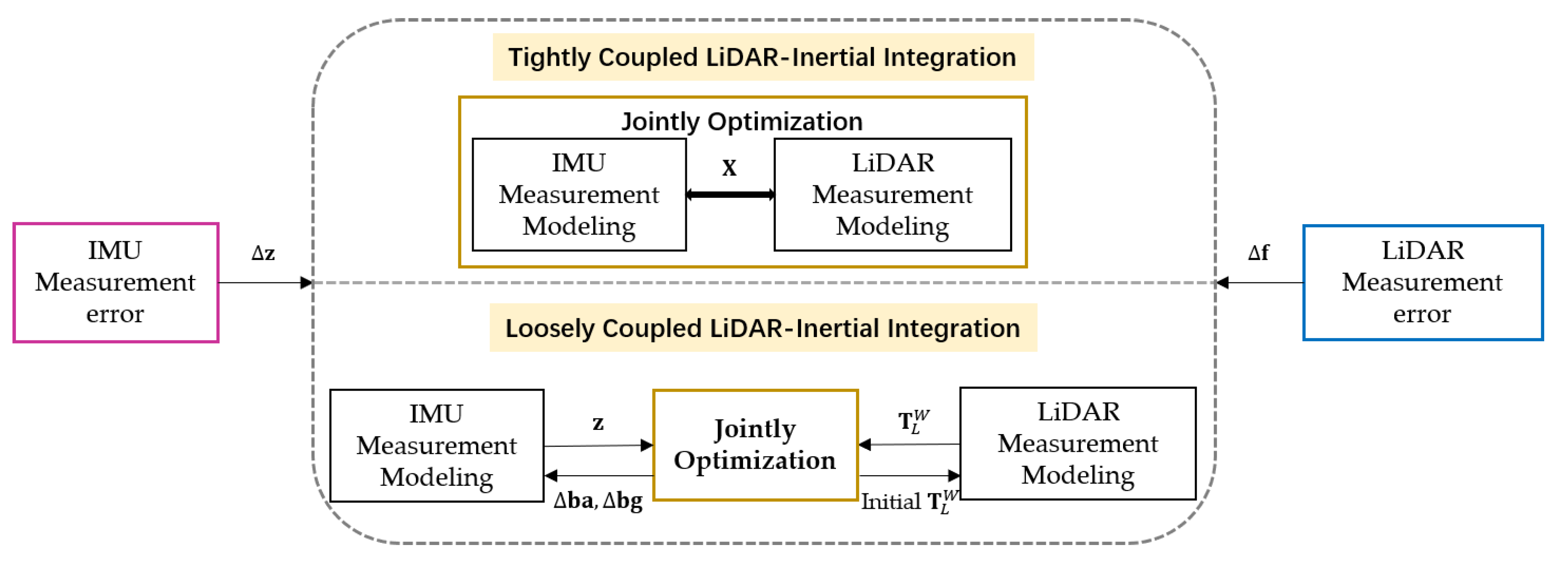
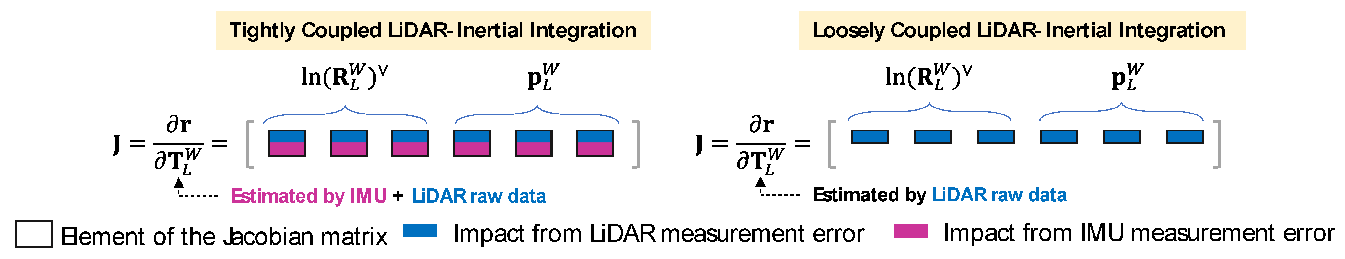
4. Performance Upper Bound Analysis of Tightly Coupled and Loosely Coupled LiDAR-Inertial Integration

In this section, the error propagation process of both the LC and TC LiDAR/inertial integration would be presented from the theoretical perspective, in an attempt to show the performance upper bounds of LiDAR scan-to-map registration in different pipelines given the same sensor measurements.

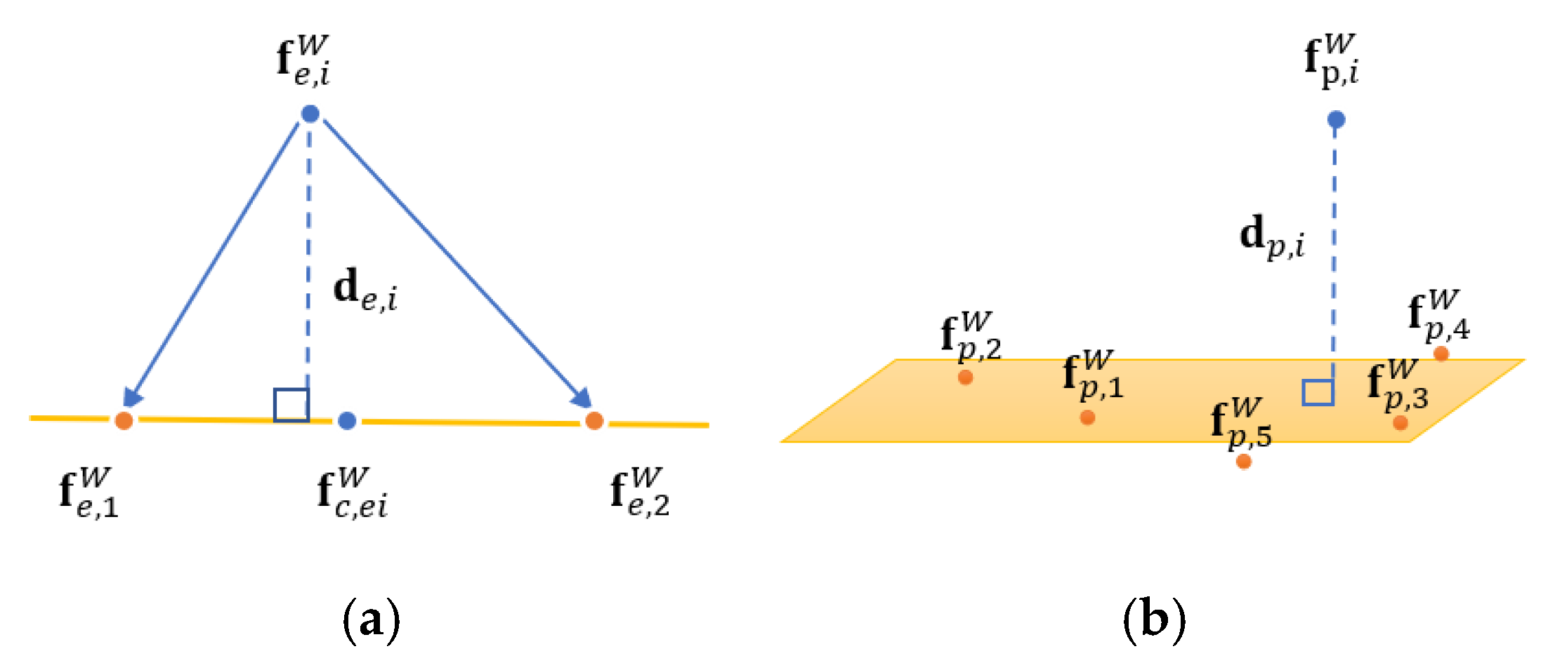
4.1. Error Propagation of LiDAR Measurement in TC-LIO

The general cost function of factor graph-based TC-LIO can be expressed as:

$$X=\underset{X}{\min }\frac{1}{2}\left\{\parallel r_p{\left(X\right)\parallel }^2+{\displaystyle \sum }_{\begin{array}{c}{f}_i^{L_k}\in {ℱ}^{L_k}\\ k\in \left\{0,\cdots ,n\right\}\end{array}}\rho (\parallel r_{TC,stmr}{\left(f_i^{L_k},X\right)\parallel }_{C_{L_k}}^2)+{\displaystyle \sum }_{k\in \left\{0,\cdots ,n-1\right\}}\rho (\parallel r_{TC,ℬ}{\left(z_{B_{k+1}}^{B_k},X\right)\parallel }_{C_{B_{k+1}}^{B_k}}^2)\right\},$$

(29)

where $r_p\left(X\right)$ represents the prior factor from marginalization [16], if any. $r_{TC,stmr}(·)$ and $r_{TC,ℬ}(·)$ represents LiDAR scan-to-map registration residual and IMU pre-integration residual, respectively. Measurements from LiDAR and IMU are fused directly to constrain the state to be estimated. The raw measurements from LiDAR could reach centimeter-level accuracy. However, the measurements from IMU are much noisy with an order of magnitude lower accuracy, even if its bias is continuously corrected during optimization. Regardless of the prior factor and taking the error of the raw measurements into account, for one state $x_k$ the full Jacobian matrix $J_{TC,full}$ derived by its residual can be expressed as

$$J_{TC,full}=\left[\begin{array}{c}{J}_{r_{TC,stmr}}\\ J_{r_{TC,ℬ}}\end{array}\right]=\left[\begin{array}{c}\frac{\partial r_{TC,stmr}\left(f^{L_k}+\Delta f,x_k\right)}{\partial x_k}\\ \frac{\partial r_{TC,ℬ}\left(z_{B_{k+1}}^{B_k}+\Delta z,x_k\right)}{\partial x_k}\end{array}\right]=\left[\begin{array}{c}\frac{\partial r_{TC,stmr}\left(f^{L_k},x_k\right)}{\partial x_k}+\frac{\partial r_{TC,stmr}\left(\Delta f,x_k\right)}{\partial x_k}\\ \frac{\partial r_{TC,ℬ}\left(z_{B_{k+1}}^{B_k},x_k\right)}{\partial x_k}+\frac{\partial r_{TC,ℬ}\left(\Delta z,x_k\right)}{\partial x_k}\end{array}\right].$$

(30)

For simplicity simplify, $f^{L_k}$ represents all the feature points including the plane and edge points without differentiation. The Jacobian matrix of LiDAR scan-to-map registration residuals corresponding to the state is represented as one submatrix, $J_{r_{TC,stmr}}$, rather than listed at separate rows of $J_{TC,full}$. The Jacobian matrix of IMU pre-integration residuals corresponding to the state is represented as $J_{r_{TC,ℬ}}$. During the minimization of (29), $J_{TC,full}$ is iteratively evaluated. An error of IMU measurements and LiDAR measurements are represented as $\Delta z$ and $\Delta f$, respectively. The errors from both measurements are propagated to $J_{r_{TC,stmr}}$ via the state $x_k$ shared by both kinds of residuals $r_{TC,stmr}$ and $r_{TC,ℬ}$. Therefore, the final convergence of $r_{TC,stmr}$ relies on the quality of IMU and the accuracy of its noise modeling. Unfortunately, the noise of the IMU drifts and is hard to obtain, even if the noise is estimated or corrected simultaneously by the LiDAR scan-to-map registration. As a result, the potential for the high accuracy of the raw LiDAR measurements is not fully relaxed. A similar argument is also presented in a study [37] where a similar coarse-to-fine LiDAR/visual integration scheme is proposed. It maintains that there is a significant difference between the accuracy level of the visual measurements and the LiDAR measurements, and therefore, the direct and joint optimization of the residuals derived from two kinds of observations can not relax the potential for LiDAR measurements.

The illustration of the measurement error propagation for TC-LIO is shown in Figure 6, in which the error of IMU measurements is directly absorbed to the LiDAR scan-to-map registration due to the tightly coupled integration.

4.2. Error Propagation in LiDAR Measurement Modeling of LC-LIO

The general cost function of factor graph-based LC-LIO can be expressed as Equation (7). During the minimization of Equation (7), for one state $x_k$ the full Jacobian matrix $J_{LC,full}$ derived by its residual can be expressed as:

$$J_{LC,full}=\left[\begin{array}{c}{J}_{r_{LC,ℒ}}\\ J_{r_{LC,ℬ}}\end{array}\right]=\left[\begin{array}{c}\frac{\partial r_{LC,ℒ}\left(T_{L_k}^W+\Delta T_{L_k}^W,x_k\right)}{\partial x_k}\\ \frac{\partial r_{LC,ℬ}\left(z_{B_{k+1}}^{B_k}+\Delta z,x_k\right)}{\partial x_k}\end{array}\right]=\left[\begin{array}{c}\frac{\partial r_{LC,ℒ}\left(T_{L_k}^W,x_k\right)}{\partial x_k}+\frac{\partial r_{LC,ℒ}\left(\Delta T_{L_k}^W,x_k\right)}{\partial x_k}\\ \frac{\partial r_{LC,ℬ}\left(z_{B_{k+1}}^{B_k},x_k\right)}{\partial x_k}+\frac{\partial r_{LC,ℬ}\left(\Delta z,x_k\right)}{\partial x_k}\end{array}\right],$$

(31)

where, $T_{L_k}^W$ represents the pose of LiDAR solved by the iterative optimization of scan-to-map registration in a separate module and $\Delta T_{L_k}^W$ represents the error of $T_{L_k}^W$. To make a distinction between TC demonstrated in Section 4.1 and LC, the subscript ‘’LC’’ is added for residual items $r_{ℒ}(·)$ and $r_{ℬ}(·)$ in Equation (7). The registration minimizes the point-to-line and point-to-map matching residuals, as shown in Equations (22) and (24):

$$T_{L_k}^W=\underset{T_{L_k}^W}{\min }\frac{1}{2}\left\{{\displaystyle \sum }_{f_i^{L_k}\in {ℱ}^{L_k}}\parallel r_{LC,stmr}{\left(f_i^{L_k},T_{L_k}^W\right)\parallel }^2\right\}=\underset{T_{L_k}^W}{\min }\frac{1}{2}\{{\displaystyle \sum }_{f_{e,i}^{L_k}\in {ℰ}^{L_k}}\parallel r_{e,i}{\left(f_{e,i}^{L_k},T_{L_k}^W\right)\parallel }^2+{\displaystyle \sum }_{f_{p,i}^{L_k}\in {𝒫}^{L_k}}\parallel r_{p,i}{\left(f_{p,i}^{L_k},T_{L_k}^W\right)\parallel }^2\}.$$

(32)

During the minimization, the Jacobian matrix $J_{r_{LC,stmr}}$ of the matching residuals $r_{LC,stmr}(·)$ corresponding to $T_{L_k}^W$ can be expressed as:

$$J_{r_{LC,stmr}}=\left[\frac{\partial r_{LC,stmr}\left(f^{L_k}+\Delta f,T_{L_k}^W\right)}{\partial T_{L_k}^W}\right]=\left[\frac{\partial r_{LC,stmr}\left(f^{L_k},T_{L_k}^W\right)}{\partial T_{L_k}^W}+\frac{\partial r_{LC,stmr}\left(\Delta f,T_{L_k}^W\right)}{\partial T_{L_k}^W}\right].$$

(33)

where, $\Delta T_{L_k}^W$ are obtained by the error of LiDAR measurements only. In other words, the LiDAR scan-to-map registration cannot be directly affected by the error arising from IMU measurements.

The illustration of the measurement error propagation for LC-LIO is shown in Figure 6, and the LiDAR scan-to-map registration is decoupled from IMU measurements. Moreover, the high-frequency IMU measurements provide an initial guess of the pose estimation in time for the registration, which is significantly beneficial to obtaining an ideal optimal solution.

4.3. Performance Upper Bound Analysis

LiDAR scan-to-map registration is modeled as an iterative nonlinear optimization problem both in TC-LIO and LC-LIO as mentioned above. The difference is that it is jointly optimized with IMU measurements in TC-LIO as Equation (29) while separately optimized in LC-LIO as (32). Based on the L-M algorithm, the iteratively estimated pose $T_L^W$ during the registration whether in TC-LIO or LC-LIO can be expressed as follows [3]:

$$T_{L_k}^W=T_{L_k}^W{\left(J_{r_{(·),stmr}}{}^T{J}_{r_{(·),stmr}}+\lambda Diag\left(J_{r_{(·),stmr}}{}^T{J}_{r_{(·),stmr}}\right)\right)}^{-1}\left(-J_{r_{(·),stmr}}{}^T{r}_{(·),stmr}\right),$$

(34)

where $(·)$ represents TC or LC. $\lambda$ represents the damping factor of the L-M algorithm. $Diag\left(J_{r_{(·),stmr}}{}^T{J}_{r_{(·),stmr}}\right)$ represents matrix constructed by diagonal elements of the matrix $J_{r_{(·),stmr}}{}^T{J}_{r_{(·),stmr}}$.

For the TC-LIO, the LiDAR scan-to-map registration and the IMU measurement modeling share the same motion state. $T_{L_k}^W$ is obtained via the jointly optimized state $x_k$ and the pre-calibrated extrinsic transformation matrix between the IMU and the LiDAR. During the registration, the Jacobian matrix $J_{r_{TC,stmr}}$ and the residual $r_{TC,stmr}$ are both decided by $x_k$ as demonstrated in Equations (29) and (30). As shown in Figure 7, apart from the potential error from LiDAR measurements, when computing the residual and the Jacobian matrix, the error of IMU is also involved in the shared state which would affect the solution to $T_{L_k}^W$ in Equation (34). For LC-LIO, the two models are separated. The iterative optimization of LiDAR scan-to-map registration is free from IMU measurement modeling as demonstrated in Equation (32). It utilizes the high accuracy of LiDAR measurement and the high-frequency pose estimation from IMU as the initial guess. In short, in TC-LIO the performance upper bound of the LiDAR scan-to-map registration is blocked by the additional error of IMU. While in LC-LIO, it is mainly decided by the accuracy of the LiDAR measurements.

5. Experimental Results

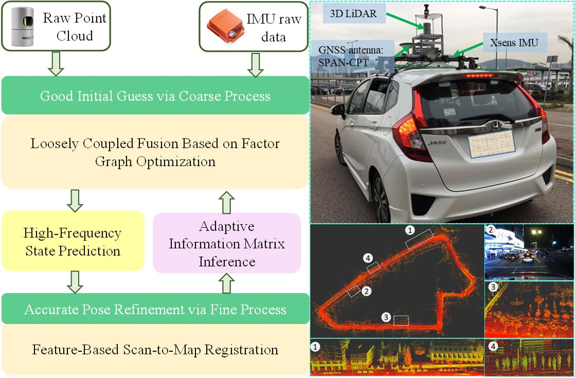
5.1. Experiment Setup

5.1.1. Sensor Setups

Two experiments were conducted in typical urban canyons in Hong Kong with the aim of verifying the effectiveness of the proposed method. Meanwhile, the datasets [38] in this study were open to the community for further algorithm development and verification. The detail of the data collection vehicle can be found through the site of our open-sourced UrbanNav dataset (https://github.com/weisongwen/UrbanNavDataset, accessed on 15 June 2021). A Velodyne HDL-32E 3D LiDAR sensor is employed to collect 3D point clouds at a frequency of 10 Hz. An Xsens Ti-10 IMU was adopted to acquire acceleration and angular velocity at a frequency of 200 Hz. The NovAtel SPAN-CPT, a GNSS (GPS, GLONASS and Beidou) RTK/INS (fiber-optic gyroscopes, FOG) integrated navigation system was employed to provide ground truth of the pose. All the data were collected and synchronized with the open-source robot operation system (ROS) [39]. The transformation matrixes among different coordinates of the sensors were calibrated in advance. The proposed methods were implemented in C++ and executed on a laptop equipped with an Intel i7-9750H CPU and 24.0 GB RAM using the ROS in Ubuntu Linux.

5.1.2. Evaluation Metrics

According to the extensive evaluations of the existing LiDAR/inertial integration pipelines [16], the LiLi-OM achieved the best performance among these existing TC solutions (such as LIO-SAM [13] and Lio-mapping [11]). Therefore, the comparison was directly drawn on the proposed LC-LIO and LiLi-OM. As LC-LIO was a pure odometry algorithm, the loop closure function of LiLi-OM was disabled during the evaluation. It could be noted that both estimated trajectories were aligned with the ground truth with EVO [40], which was a popular toolkit for the performance evaluation of odometry estimation. For the quantitative evaluation, the Relative Pose Error (RPE) was calculated using EVO [40]. It compares the relative pose in a fixed time interval of the estimated ones with that of the ground-truth [41]. Given a sequence of estimated pose $\mathsf{{\rm E}}=\left\{T_{est,1}, T_{est,2}, \dots ,T_{est,n}\right\}$ and the corresponding ground-truth $\mathrm{G}=\left\{T_{gt,1}, T_{gt,2}, \dots ,T_{gt,n}\right\}$, the RPE between the $i$-th and the $j$-th pose can be expressed as:

$$\mathsf{\delta }{T}_{i,j}={(T_{gt,i}{}^{-1}{T}_{gt,j})}^{-1}(T_{est,i}{}^{-1}{T}_{est,j}).$$

(35)

The rotation part and the translation part of $\mathsf{\delta }{T}_{i,j}$ are regarded as the Relative Rotation Error (RRE) and the Relative Translation Error (RTE), respectively. The following three pipelines can be compared to show the effectiveness of the proposed method:

(1)

LiLi-OM [16]: Tightly-coupled integration of LiDAR/inertial method.

(2)

LC-LIO-FC: The proposed coarse-to-fine loosely-coupled integration of LiDAR/inertial with fixed covariance.

(3)

LC-LIO-AC: The proposed coarse-to-fine loosely-coupled integration of LiDAR/inertial with adaptive covariance based on Equation (28).

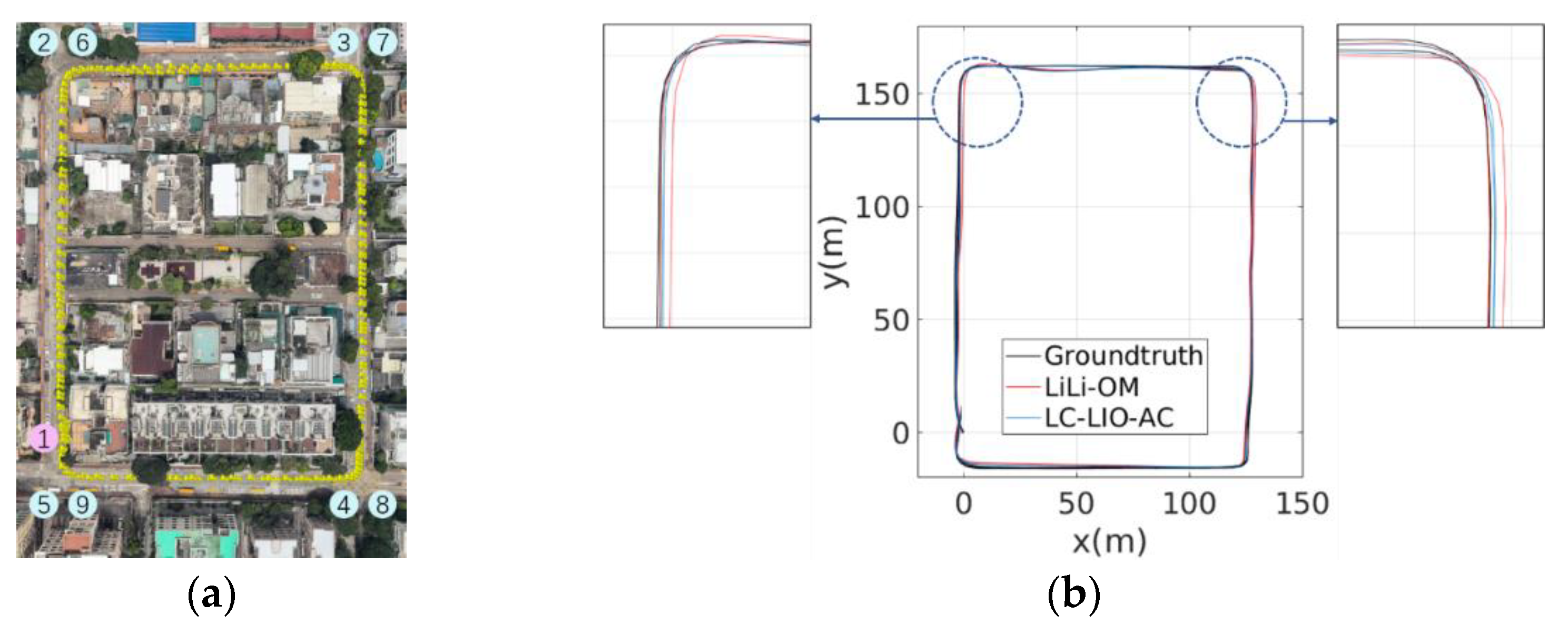
5.2. Experiments in Urban Canyon 1: The HK-Data20200314 Dataset

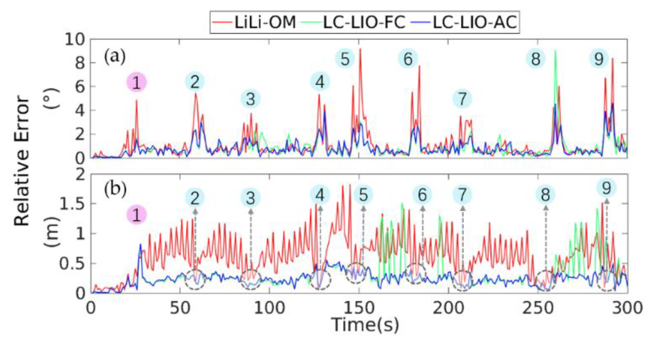
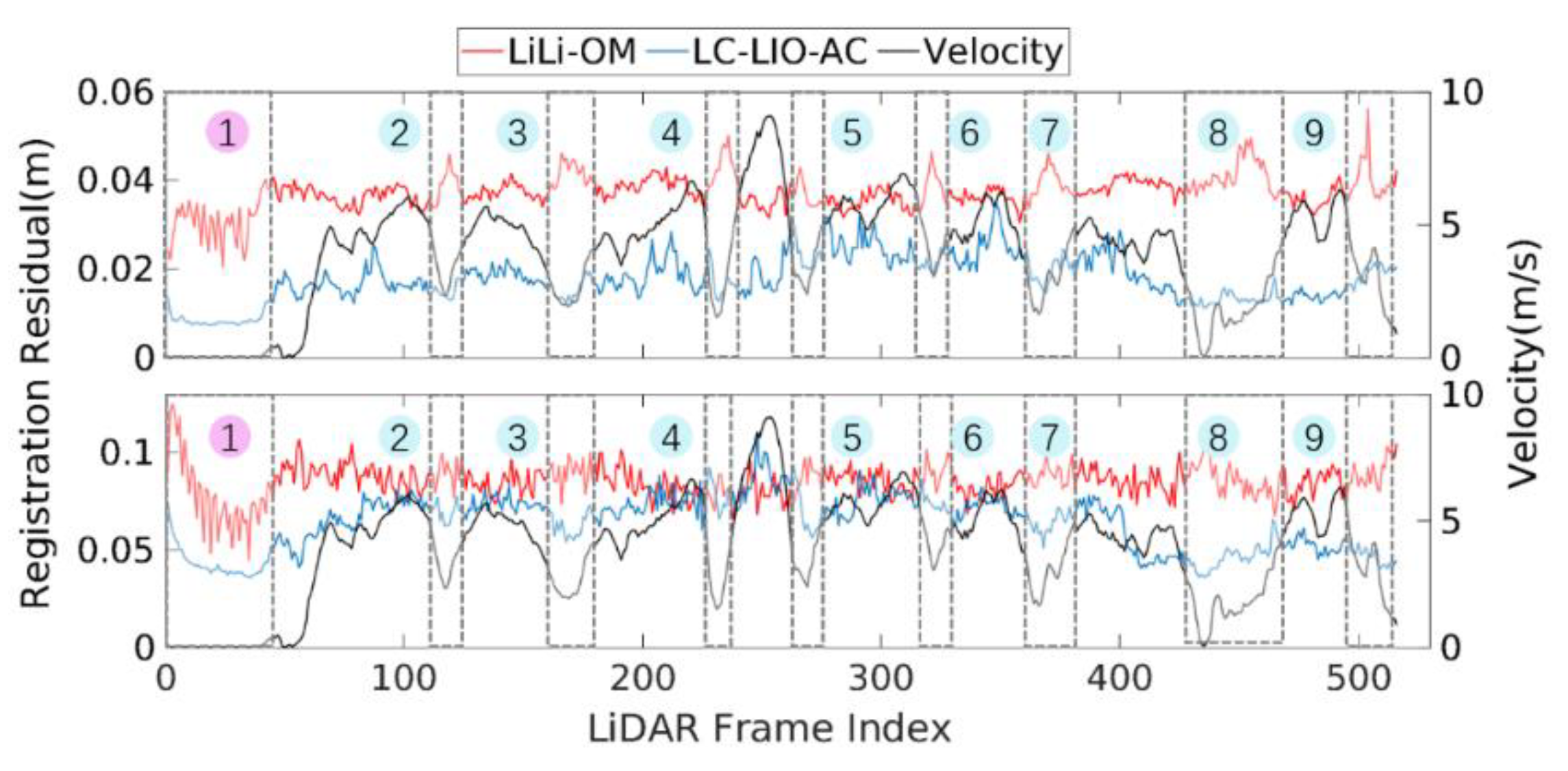
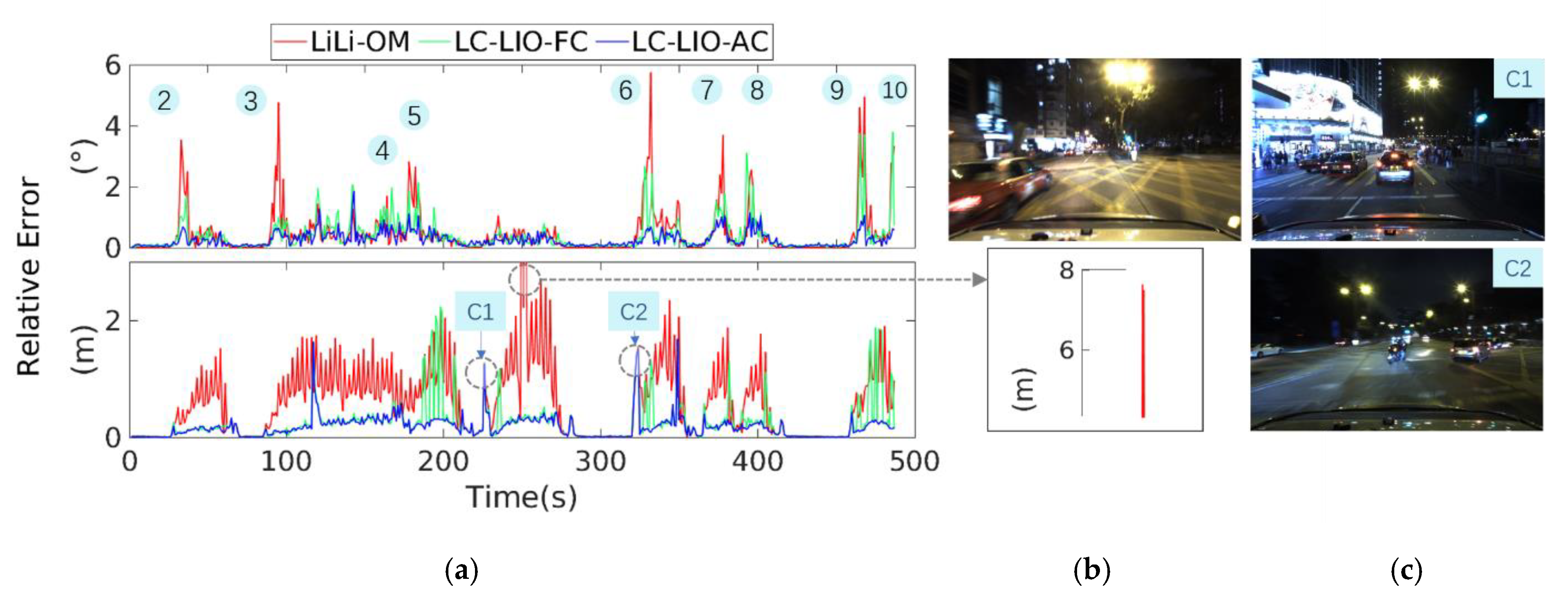
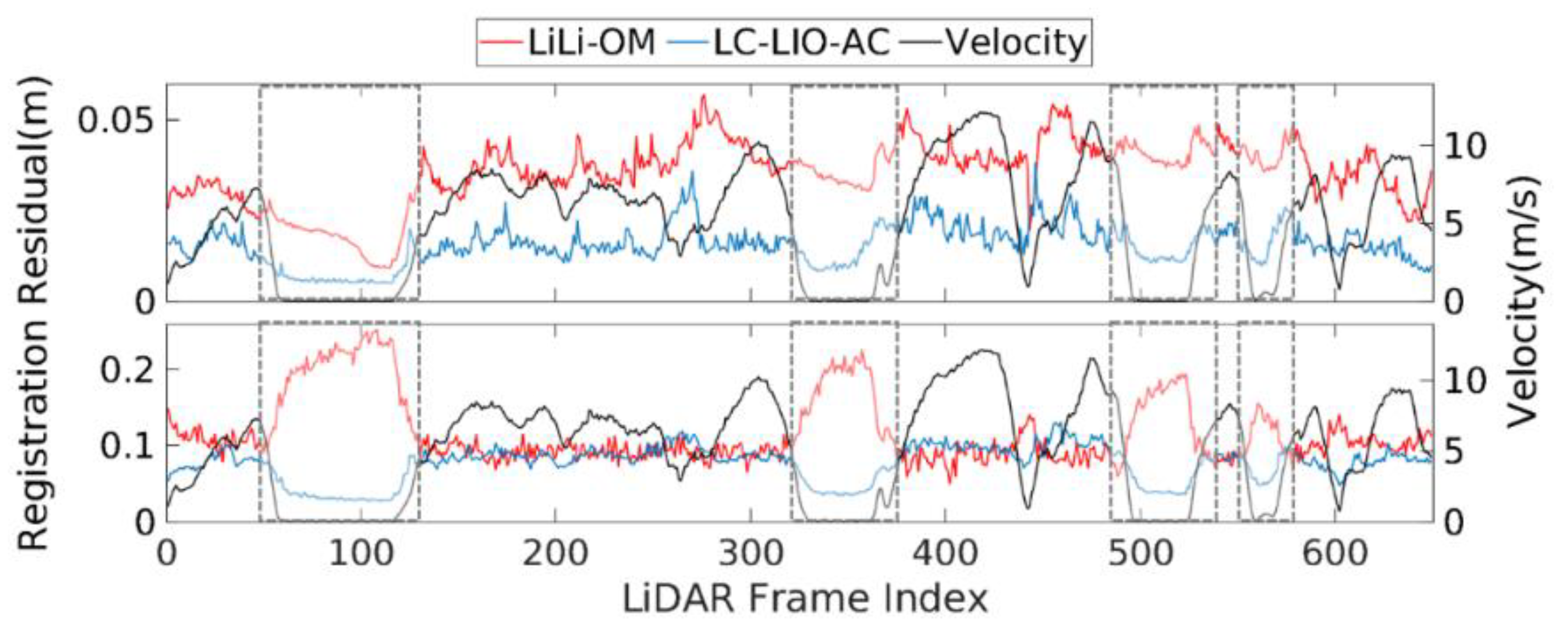
5.2.1. Performance Analysis

The HK-Data20200314 is collected in Kowloon Tong which is a suburban area with lower buildings and less dynamic objects compared with the HK-Data20190428. The total length is 1.21 km.

Table 1. RPE of LiLi-OM, LC-LIO-FC and LC-LIO-AC produced by EVO [40] in the urban canyon 1. The bold values represents best precision.

Dataset	Method	Relative Rotation Error (°)		Relative Translation Error (m)
		Mean Value	RMSE	Mean Value	RMSE
Urban Canyon 1 (HK-Data20200314)	LiLI-OM	1.133	1.762	0.605	0.693
	LC-LIO-FC	0.885	1.249	0.271	0.348
	LC-LIO-AC	0.800	1.115	0.233	0.262

shows the performance results of the RPE of LiLi-OM, LC-LIO-FC and LC-LIO-AC in the urban canyon 1. In order to improve the repeatability, five tests are carried out and an average is calculated as the final RPE result. For LiLi-OM, the Root Mean Squared Error (RMSE) of RRE is 1.762$°$ with a mean value of 1.133$°$. RMSE of RTE is 0.693 m with a mean of 0.605 m. The percentage improvement of RMSE can be defined as subtracting the smaller ones from the larger ones and then dividing the latter by the difference. By LC-LIO-FC, a 30% improved RMSE of 1.249$°$ with a mean value of 0.885$°$ for RRE and a 50% improved RMSE of 0.348 m with a mean of 0.271 m for RTE can be achieved. The improvement indicates the superiority of the proposed LC framework. The best precision is achieved by LC-LIO-AC as marked in bold font. After applying the adaptive covariance estimation, the RMSE of RRE decreases to 0.8$°$, with a mean value of 1.115$°$, and the RMSE of RTE decreases to 0.233 m, with a mean value of 0.262 m. Due to the fact that there are few dynamic objects and adequate structured features, LiDAR scan-to-map registration is generally reliable. As a result, the precision of LC-LIO-AC is slightly better than that of LC-LIO-FC. However, the improvement still shows the effectiveness of the adaptive covariance estimation.

Figure 8 presents the estimated trajectories from LC-LIO-AC and LiLi-OM and the ground-truth in the urban canyon 1. As shown in Figure 8b when the first lap is traversed, the two algorithms can achieve similar trajectories which almost overlap with the ground truth. When the second lap is traversed, the trajectory estimated by LC-LIO-AC performs better. While the trajectory from LiLi-OM deviates from the ground truth worth especially at the top two turns.

Figure 9 presents the RPE of LiLi-OM, LC-LIO-FC and LC-LIO-AC on the entire trajectory of one experiment. As shown in Figure 9a, the RRE of LiLi-OM is significantly larger than that of LC-LIO-FC at most selected control points marked by numbers, which correspond to the place represented in Figure 8a. It is more difficult to perform LiDAR scan-to-map registration at turns due to the dramatic changes in rotation. Therefore, the relative rotation error at turns is larger than that on straight roads. However, the LC-LIO-FC outperforms LiLi-OM at most turns on the ground that it can register each LiDAR frame more precisely in the rotation domain with the assistance of LC IMU predictions, which demonstrates the effectiveness of the proposed LC framework. There is further improvement of the RRE especially at the nine marked challenging places of LC-LIO-AC compared with LC-LIO-FC. The adaptive covariance estimation contributes to the defense of degenerate LiDAR scan-to-map registration.

Figure 9b shows the RTE of the three methods with the places at gray circles indicating comparative accuracy. During IMU pre-integration, the translation is determined by rotation as shown in Equations (12)–(16). For LiLi-OM, LiDAR scan-to-map registration is directly coupled with IMU pre-integration. The RTE of LiLi-OM is notably larger than that of LC-LIO-FC on account of its larger RRE. In other words, a larger error at the turn results in more deviation of the estimated trajectory from the ground truth after that turn. The RTE of LC-LIO-AC is improved significantly at several places compared with LC-LIO-FC due to the assistance of adaptive covariance estimation. However, when at the eight turns, as marked by gray circles in Figure 9b, the RTE of the three methods are comparable. Due to the fact that the road of this dataset is narrow, the vehicle moves more slowly at turns and the translation is small. Consequently, the RTE of the three methods is always smaller at such places.

5.2.2. Quantitative Analysis of the Performance Upper Bound in TC-LIO and LC-LIO

For LiDAR scan-to-map registration, a smaller matching residual between feature points on the scan and the map demonstrates better convergence and thus resulting in a more optimal estimation [8]. To demonstrate that the error of IMU would block the performance of the LiDAR scan-to-map registration for TC-LIO while it is opposite for LC-LIO, the comparison has been drawn on the final registration residuals for each frame of LiLi-OM and LC-LIO-AC that are correspondent in time. It could be observed that the final registration residuals of both edge points and plane points are defined as the average registration residual of all the registered points in the corresponding categories when the registration converges. Therefore, it can be expressed as:

$$r_{{ℱ}^{L_k},(·)}=\frac{1}{N_{(·)}}{\displaystyle \sum }_{f_{(·),i}^{L_k}}\sqrt{\rho \left(\parallel r_{ℒ}{\left(f_{(·),i}^{L_k},T_{L_k}^W\right)\parallel }^2\right)}.$$

(36)

where $(·)$ represents $e$ for edge points or $p$ for plane points. $r_{{ℱ}^{L_k},(·)}$ represents the final registration residuals of the edge points or plane points on the currently involved LiDAR frame ${ℱ}^{L_k}$. $N_{(·)}$ represents the total number of edge points or plane points. $T_{L_k}^W$ represents the pose of ${ℱ}^{L_k}$ estimated by the registration. For the TC framework LiLi-OM, $T_{L_k}^W$ can be obtained through $x_k$ optimized using measurements from both LiDAR and IMU as shown in (29). For the LC framework LC-LIO-AC, $T_{L_k}^W$ can be obtained via iterative minimizing the scan-to-map registration residual with measurements from LiDAR alone as shown in Equation (32). $\rho$ represents the Cauchy Kernel defined as (9). In LiLi-OM it can be implemented by Ceres modifying the residual iteratively during the TC optimization which cannot be ignored. Consequently, it is taken into account here.

As shown in Figure 10, the average registration residual of plane points plotted in the top panel is generally smaller than that of edge points plotted in the bottom panel, in that the number of plane points is larger than that of edge points in space. It makes the registration more reliable for plane points. More importantly, the average registration error of both plane points and edge points generated by LiLi-OM is larger than those of LC-LIO-AC. The vehicle moves more slowly at the places marked in gray boxes as depicted by the black line representing velocity in Figure 10. The slow motion ensures precise scan-to-map registration as the overlaps among LiDAR frames are considerable. The registration residuals of LiLi-OM at such times are notably larger than LC-LIO-AC. It is because LC-LIO-AC preserves the advantage and is free from disturbance of IMU measurements thus achieves locally lower registration residuals at such times. On the contrary, in LiLi-OM, as a TC-LIO, the hard shaking and noisy IMU measurements cause disturbance to LiDAR scan-to-map registration. It is concluded that the performance upper bound of LiDAR scan-to-map registration in TC-LIO is worse than that of LC-LIO because of the IMU error propagated in as an encumbrance.

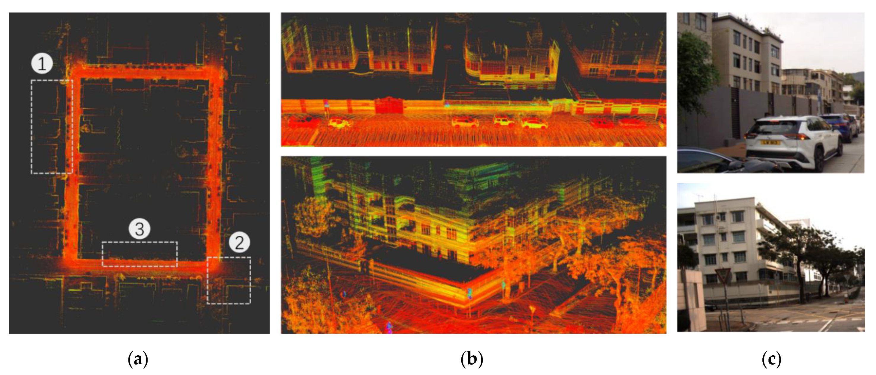
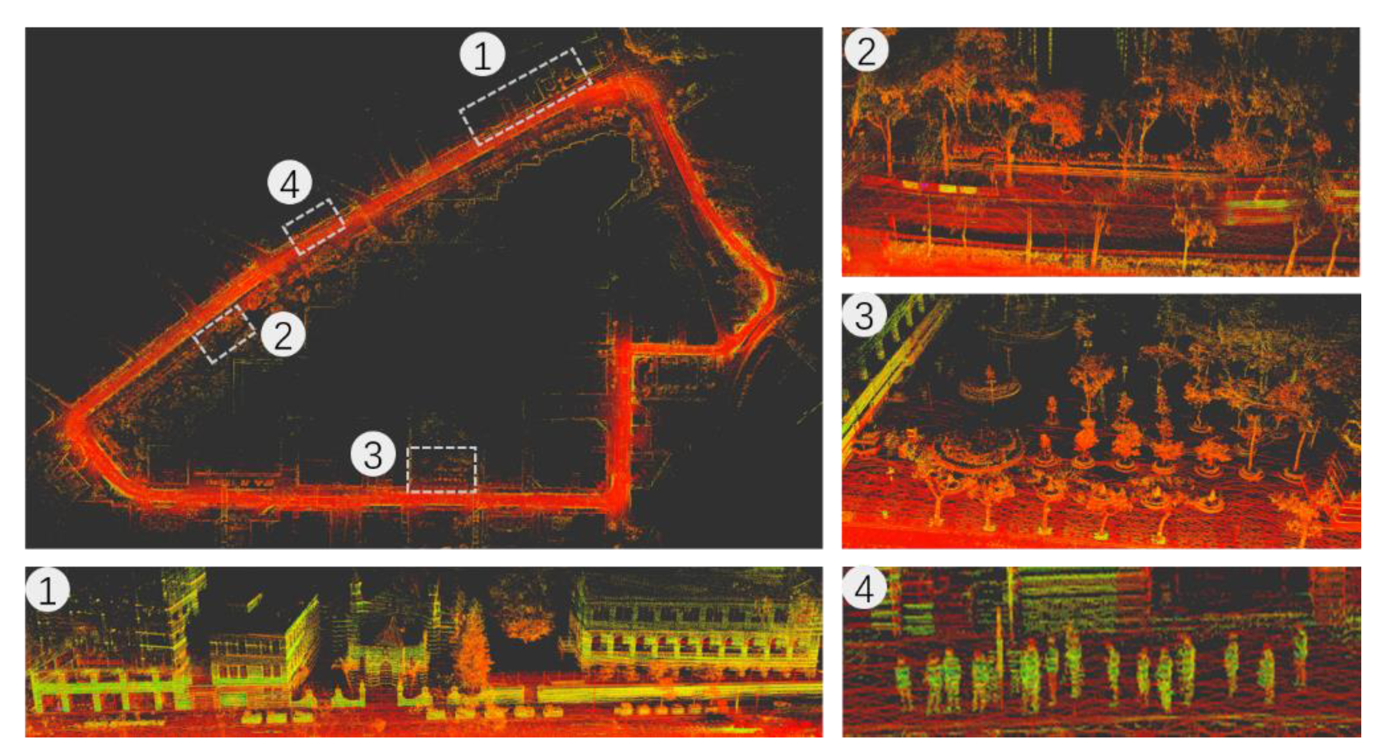
5.2.3. Mapping Result

Figure 11a shows the map generated by LC-LIO-AC in urban canyon 1 rendered with intensity value. The top and bottom panels shown in Figure 11b represent the zoomed-in maps of the first place and the second place marked in Figure 11a, respectively. The map preserves elaborated structural details of the surroundings even at turns. In addition to accurate positioning results, LC-LIO-AC produces a globally consistent point map composed of point clouds registered by LiDAR scan-to-map registration.

As shown in Figure 12, there is an obvious contrast between both maps generated by LC-LIO-AC with and without the coarse-to-fine process. When the vehicle passes the same place the second time, the map generated by LC-LIO-AC with the coarse-to-fine process is more clear while that generated by LC-LIO-AC without the coarse-to-fine process suffers blur. The proposed coarse-to-fine process of LC-LIO-AC, which provides an initial guess to the LiDAR scan-to-map registration as demonstrated in Equation (21), contributes to the refinement of the globally consistent map thus the robustness and the repeatability can be guaranteed. As for the LC-LIO-AC without the feedback from the coarse-to-fine process, the pose produced by the last scan-to-map registration is employed as the initial guess. In an open area shown in Figure 12 where the vehicle moves fast, there is a significant motion difference between the last and the current frame. Taking the pose of the last frame as the initial guess for the current one will lead to degeneration in the long run.

5.3. Experiments in the Urban Canyon 2: The HK-Data20190428 Dataset

5.3.1. Performance Analysis

The HK-Data20190428 is collected in a typical urban canyon near Tsim Sha Tsui in Hong Kong which is complex containing numerous skyscrapers, dynamic objects and vegetation. The vehicle goes back to the start point and continues on the same path as previous for a while. The total length reaches up to 2.01 km. Due to the heavy traffic, stop-and-go driving is unavoidable for the vehicle. The superiority of the proposed LC-LIO is fully developed.

Table 2. RPE of LiLi-OM, LC-LIO-FC and LC-LIO-AC produced by EVO [40] on urban canyon 2. The bold values represents best precision.

Dataset	Method	Relative Rotation Error (°)		Relative Translation Error (m)
		Mean Value	RMSE	Mean Value	RMSE
Urban Canyon 2 (HK-Data20190428)	LiLi-OM	0.458	0.878	0.609	0.891
	LC-LIO-FC	0.421	0.671	0.249	0.431
	LC-LIO-AC	0.331	0.478	0.182	0.267

shows the RPE of LiLi-OM, LC-LIO-FC and LC-LIO-AC. For LiLi-OM, the RMSE of RRE is 0.878$°$ with a mean value of 0.458$°$. The RMSE of RTE is 0.891m with a mean value of 0.609 m. For LC-LIO-FC, the RMSE of RRE is 0.671$°$ with a mean value of 0.421$°$. The RMSE of RTE is 0.431 m with a mean value of 0.249 m. The improvement indicates the superiority of the proposed LC framework. The best precision can be achieved by LC-LIO-AC as marked in bold font. The RMSE of the RRE and RTE is 45% and 70% better, respectively, compared to LiLi-OM. They are 40% and 30% better compared to LC-LIO-FC. The effectiveness of the adaptive covariance estimation is validated.

Figure 13 depicts the ground truth and the estimated trajectories from LC-LIO-AC and LiLi-OM in the urban canyon 2. As shown in Figure 13b, the trajectory estimated by LC-LIO-AC matches the ground truth better than LiLi-OM, especially at turns. Figure 14 presents the RRE and RPE of the three methods for one experiment. Exactly as the analysis in Section 5.2.1, the RRE is larger at turns than on straight roads. Nevertheless, LC-LIO-FC outperforms LiLi-OM at most turns owing to the LC IMU predictions. With the assistance of adaptive covariance estimation, which reduces the weight of the scan matching factor when the LiDAR scan-to-map registration residual is large under challenging scenes, LC-LIO-AC outperforms LC-LIO-FC at all turns. The larger rotation error leads to a larger translation error again. Due to the wide street and the hurried traffic in urban canyon 2, the vehicle moves fast even at turns. Different from the condition in urban canyon 1, the RTE of LiLi-OM is still larger at turns.

In Figure 14, the zoomed-in detail of the RTE of LiLi-OM reaches up to eight meters. As shown in Figure 14b, an open intersection exists and a fast-moving taxi is passing by. The dynamic object so close complicates the LiDAR scan-to-map registration and finally results in large registration errors. LC-LIO-FC and LC-LIO-AC survive at this scene as LC fusion is more robust in comparison to TC fusion when the registration almost fails. The fused sensors in LC fusion are relatively independent during the state estimation while those in TC fusion are tightly linked. To be specific, at such scenes, in TC fusion one healthy IMU pre-integration factor directly confronts hundreds of thousands of unhealthy factors with large errors during optimization. While in the proposed LC fusion, there is at least one IMU pre-integration factor versus the single unhealthy scan-matching factor which functions to overcome the occasional failure of LiDAR scan-to-map registration.

It is worth mentioning that the LiLi-OM achieves similar accuracy with the proposed LC-LIO-FC and LC-LIO-AC in some epochs. As shown in Figure 14a,c, at place C1 with many pedestrians and place C2 with fast-moving objects around, all three methods achieve large RTE among which LiLi-OM performs slightly better. It indicates that the fusion mechanism could not improve the problem of LiDAR scan-to-map registration itself at its root which is essentially a problem of data association [42] with enough stable feature points acquisition being the key prerequisite. The few sparse scenarios where stable feature points are hardly guaranteed lead to the degeneration of the LiDAR scan-to-map registration. As the three methods adopt the same feature extraction strategy presented by [3], LC-LIO-FC and LC-LIO-AC fail to turn the tide at such extremely challenging scenes. Furthermore, the LiLi-OM performs slightly better is in that a TC integration scheme could directly employ both the IMU and LiDAR measurements to constrain the pose of the vehicle which enhances the robustness against the degeneration scenarios. For that reason, it can be argued that a promising solution is to detect the context of the environment (e.g., stable features abundant or sparse area) to achieve mutual complementarity by further combining loosely and tightly coupled integrations alternatively.

5.3.2. Quantitative Analysis of the Performance Upper Bound in TC-LIO and LC-LIO

The average LiDAR scan-to-map registration residuals of plane points and edge points generated by LiLi-OM and LC-LIO-AC on corresponding LiDAR frames in the urban canyon 2 are plotted in Figure 15. On the whole, the residual of LC-LIO-AC is smaller than that of LiLi-OM on both types of feature points. The performance of LiDAR scan-to-map registration in LC-LIO-AC is better than that of LiLi-OM. As shown in the gray boxes, when the vehicle stops to wait for the green light with the corresponding velocity depicted by the black line being zero, the registration residuals of LC-LIO-AC are significantly smaller than those of LiLi-OM, especially obvious for edge points. As the scenario is high-dynamic containing pedestrians and vehicles, the edge points are more fragile to the IMU bias which would cause damage to LiDAR scan-to-map registration.

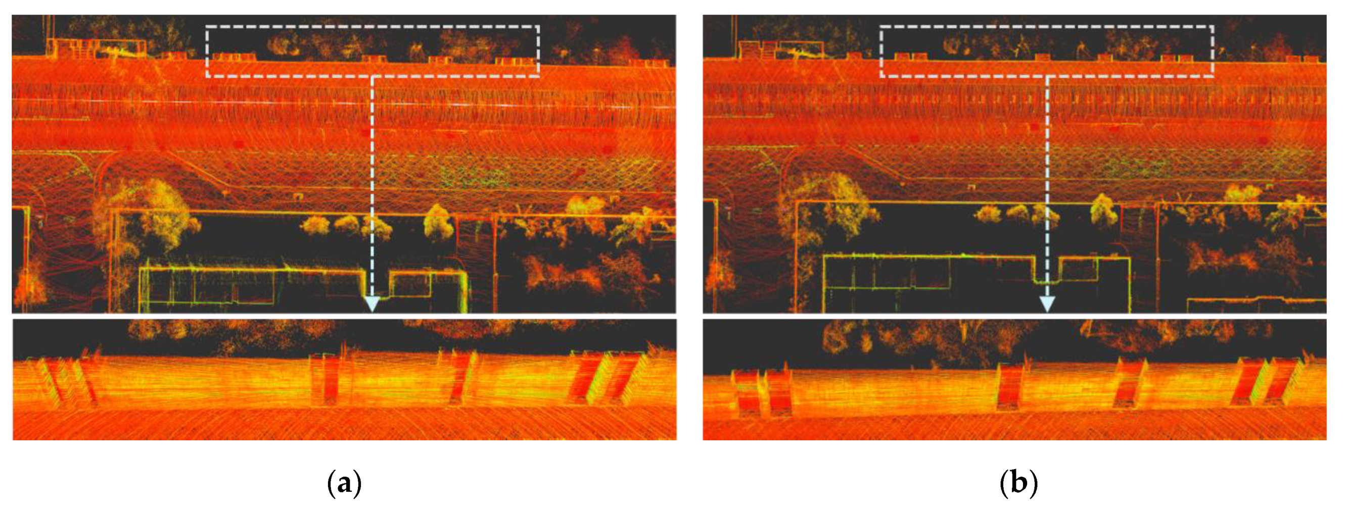
5.3.3. Mapping Result of the Proposed LC-LIO

The proposed LC-LIO-AC finished the global reconstruction of the real world in the urban canyon 2 with the generated map shown in Figure 16. The scanned buildings, vegetation and the pedestrian are all registered accurately in a globally consistent map.

6. Conclusions and Future Perspectives

In this paper, the coarse-to-fine LC-LIO has been developed to perform motion estimation and mapping in urban canyons for autonomous navigation. The LiDAR scan-to-map registration, which is the fine process, can produce a globally consistent map and conduct a precision motion estimation with the timely and high-frequency initial guess provided by the LC integrated IMU based on factor graph optimization as the coarse process. Our algorithm is capable of providing real-time, long-term and accurate motion states and point cloud maps. Furthermore, the superiority of the proposed pipeline compared with TC fusion has been verified from the perspective of theoretical error propagation. The experiment results on typical urban canyons in Hong Kong indicate that the proposed LC-LIO outperforms LiLi-OM in accuracy, which is currently the state-of-the-art TC-LIO scheme.

In the future, the absolute positioning from the Global Navigation Satellite System (GNSS) real-time kinematic positioning (RTK) will be integrated with the proposed LC-LIO pipeline to achieve the drift-free motion estimation and map. Moreover, according to recent findings [43,44,45], the generated map of the surrounding area can effectively detect the GPS outlier measurements in urban canyons. Therefore, it deserves to make an exploration on the potential of the proposed LC-LIO pipeline in improving the GPS positioning.

References

1. Wen, W.; Zhang, G.; Hsu, L.-T. GNSS NLOS exclusion based on dynamic object detection using LiDAR point cloud. IEEE Trans. Intell. Transp. Syst. 2019, 22, 853–862. [Google Scholar] [CrossRef]
2. Breßler, J.; Reisdorf, P.; Obst, M.; Wanielik, G. GNSS positioning in non-line-of-sight context—A survey. In Proceedings of the 2016 IEEE 19th International Conference on Intelligent Transportation Systems (ITSC), Rio de Janeiro, Brazil, 1–4 November 2016; pp. 1147–1154. [Google Scholar]
3. Zhang, J.; Singh, S. Low-drift and real-time lidar odometry and mapping. Auton. Robot. 2017, 41, 401–416. [Google Scholar] [CrossRef]
4. Wen, W.; Zhou, Y.; Zhang, G.; Fahandezh-Saadi, S.; Bai, X.; Zhan, W.; Tomizuka, M.; Hsu, L.-T. Urbanloco: A full sensor suite dataset for mapping and localization in urban scenes. In Proceedings of the 2020 IEEE International Conference on Robotics and Automation (ICRA), Paris, France, 31 May–31 August 2020; pp. 2310–2316. [Google Scholar]
5. Merriaux, P.; Dupuis, Y.; Boutteau, R.; Vasseur, P.; Savatier, X. LiDAR point clouds correction acquired from a moving car based on CAN-bus data. arXiv 2017, arXiv:1706.05886. [Google Scholar]
6. Wen, W.; Hsu, L.-T.; Zhang, G. Performance analysis of NDT-based graph SLAM for autonomous vehicle in diverse typical driving scenarios of Hong Kong. Sensors 2018, 18, 3928. [Google Scholar] [CrossRef] [Green Version]
7. Thrun, S. Probabilistic robotics. Commun. ACM 2002, 45, 52–57. [Google Scholar] [CrossRef]
8. Dellaert, F.; Kaess, M. Factor graphs for robot perception. Found. Trends Robot. 2017, 6, 1–139. [Google Scholar] [CrossRef]
9. Qin, C.; Ye, H.; Pranata, C.E.; Han, J.; Zhang, S.; Liu, M. LINS: A Lidar-Inertial State Estimator for Robust and Efficient Navigation. In Proceedings of the 2020 IEEE International Conference on Robotics and Automation (ICRA), Paris, France, 31 May–31 August 2020; pp. 8899–8906. [Google Scholar]
10. Wen, W.; Pfeifer, T.; Bai, X.; Hsu, L.T. Factor Graph Optimization for GNSS/INS Integration: A Comparison with the Extended Kalman Filter. Navigation 2020, 68, 315–331, accepted. [Google Scholar]
11. Ye, H.; Chen, Y.; Liu, M. Tightly coupled 3d lidar inertial odometry and mapping. In Proceedings of the 2019 International Conference on Robotics and Automation (ICRA), Montreal, QC, Canada, 20–24 May 2019; pp. 3144–3150. [Google Scholar]
12. Qin, T.; Li, P.; Shen, S. Vins-mono: A robust and versatile monocular visual-inertial state estimator. IEEE Trans. Robot. 2018, 34, 1004–1020. [Google Scholar] [CrossRef] [Green Version]
13. Shan, T.; Englot, B.; Meyers, D.; Wang, W.; Ratti, C.; Rus, D. LIO-SAM: Tightly-coupled Lidar Inertial Odometry via Smoothing and Mapping. In Proceedings of the IEEE/RSJ International Conference on Intelligent Robots and Systems (IROS), Las Vegas, NV, USA, 24–30 October 2020; pp. 5135–5142. [Google Scholar]
14. Kaess, M.; Ranganathan, A.; Dellaert, F. iSAM: Incremental smoothing and mapping. IEEE Trans. Robot. 2008, 24, 1365–1378. [Google Scholar] [CrossRef]
15. Balsa-Barreiro, J.; Fritsch, D. Generation of visually aesthetic and detailed 3D models of historical cities by using laser scanning and digital photogrammetry. Digit. Appl. Archaeol. Cult. Herit. 2018, 8, 57–64. [Google Scholar] [CrossRef]
16. Li, K.; Li, M.; Hanebeck, U.D. Towards high-performance solid-state-lidar-inertial odometry and mapping. IEEE Robot. Autom. Lett. 2021, 6, 5167–5174. [Google Scholar] [CrossRef]
17. Geiger, A.; Lenz, P.; Urtasun, R. Are we ready for autonomous driving? The kitti vision benchmark suite. In Proceedings of the 2012 IEEE Conference on Computer Vision and Pattern Recognition, Providence, RI, USA, 16–21 June 2012; pp. 3354–3361. [Google Scholar]
18. Shan, T.; Englot, B. Lego-loam: Lightweight and ground-optimized lidar odometry and mapping on variable terrain. In Proceedings of the 2018 IEEE/RSJ International Conference on Intelligent Robots and Systems (IROS), Madrid, Spain, 1–5 October 2018; pp. 4758–4765. [Google Scholar]
19. Demir, M.; Fujimura, K. Robust localization with low-mounted multiple LiDARs in urban environments. In Proceedings of the 2019 IEEE Intelligent Transportation Systems Conference (ITSC), Auckland, New Zealand, 27–30 October 2019; pp. 3288–3293. [Google Scholar]
20. Tang, J.; Chen, Y.; Niu, X.; Wang, L.; Chen, L.; Liu, J.; Shi, C.; Hyyppä, J. LiDAR scan matching aided inertial navigation system in GNSS-denied environments. Sensors 2015, 15, 16710–16728. [Google Scholar] [CrossRef] [PubMed]
21. Gao, X.; Zhang, T.; Liu, Y.; Yan, Q. 14 Lectures on Visual SLAM: From Theory to Practice; Publishing House of Electronics Industry: Beijing, China, 2017; pp. 236–241. [Google Scholar]
22. Huai, Z.; Huang, G. Robocentric visual-inertial odometry. In Proceedings of the 2018 IEEE/RSJ International Conference on Intelligent Robots and Systems (IROS), Madrid, Spain, 1–5 October 2018; pp. 6319–6326. [Google Scholar]
23. Barfoot, T.D. State Estimation for Robotics; Cambridge University Press: Cambridge, UK, 2017; pp. 205–284. [Google Scholar] [CrossRef]
24. Sola, J. Quaternion kinematics for the error-state Kalman filter. arXiv 2017, arXiv:1711.02508. [Google Scholar]
25. Qin, T.; Cao, S.; Pan, J.; Shen, S. A general optimization-based framework for global pose estimation with multiple sensors. arXiv 2019, arXiv:1901.03642. [Google Scholar]
26. Zhang, Z. Parameter estimation techniques: A tutorial with application to conic fitting. Image Vis. Comput. 1997, 15, 59–76. [Google Scholar] [CrossRef] [Green Version]
27. Hu, G.; Khosoussi, K.; Huang, S. Towards a reliable SLAM back-end. In Proceedings of the 2013 IEEE/RSJ International Conference on Intelligent Robots and Systems, Tokyo, Japan, 3–7 November 2013; pp. 37–43. [Google Scholar]
28. Agarwal, S.; Mierle, K. Ceres Solver. Available online: http://ceres-solver.org (accessed on 6 January 2021).
29. Moré, J.J. The Levenberg-Marquardt algorithm: Implementation and theory. In Numerical Analysis; Springer: Berlin/Heidelberg, Germany, 1978; pp. 105–116. [Google Scholar]
30. Forster, C.; Carlone, L.; Dellaert, F.; Scaramuzza, D. On-Manifold Preintegration for Real-Time Visual—Inertial Odometry. IEEE Trans. Robot. 2016, 33, 1–21. [Google Scholar] [CrossRef] [Green Version]
31. Lupton, T.; Sukkarieh, S. Visual-inertial-aided navigation for high-dynamic motion in built environments without initial conditions. IEEE Trans. Robot. 2011, 28, 61–76. [Google Scholar] [CrossRef]
32. Balsa Barreiro, J.; Avariento Vicent, J.P.; Lerma García, J.L. Airborne light detection and ranging (LiDAR) point density analysis. Sci. Res. Essays 2012, 7, 3010–3019. [Google Scholar] [CrossRef]
33. Balsa-Barreiro, J.; Lerma, J.L. Empirical study of variation in lidar point density over different land covers. Int. J. Remote Sens. 2014, 35, 3372–3383. [Google Scholar] [CrossRef]
34. Lin, J.; Zhang, F. Loam livox: A fast, robust, high-precision LiDAR odometry and mapping package for LiDARs of small FoV. In Proceedings of the 2020 IEEE International Conference on Robotics and Automation (ICRA), Paris, France, 31 May–31 August 2020; pp. 3126–3131. [Google Scholar]
35. Zhang, J.; Singh, S. Laser–visual–inertial odometry and mapping with high robustness and low drift. J. Field Robot. 2018, 35, 1242–1264. [Google Scholar] [CrossRef]
36. Zhang, J.; Kaess, M.; Singh, S. On degeneracy of optimization-based state estimation problems. In Proceedings of the 2016 IEEE International Conference on Robotics and Automation (ICRA), Stockholm, Sweden, 16–21 May 2016; pp. 809–816. [Google Scholar]
37. Zhang, J.; Singh, S. Visual-lidar odometry and mapping: Low-drift, robust, and fast. In Proceedings of the 2015 IEEE International Conference on Robotics and Automation (ICRA), Seattle, WA, USA, 26–30 May 2015; pp. 2174–2181. [Google Scholar]
38. Hsu, L.-T.; Kubo, N.; Chen, W.; Liu, Z.; Suzuki, T.; Meguro, J. UrbanNav:An open-sourced multisensory dataset for benchmarking positioning algorithms designed for urban areas (Accepted). In Proceedings of the ION GNSS+ 2021, Miami, FL, USA, 20–24 September 2021. [Google Scholar]
39. Quigley, M.; Conley, K.; Gerkey, B.; Faust, J.; Foote, T.; Leibs, J.; Wheeler, R.; Ng, A.Y. ROS: An open-source Robot Operating System. ICRA Workshop Open Source Softw. 2009, 3, 5. [Google Scholar]
40. Grupp, M. evo: Python Package for the Evaluation of Odometry and SLAM. Available online: https://github.com/MichaelGrupp/evo (accessed on 1 March 2021).
41. Zhang, Z.; Scaramuzza, D. A tutorial on quantitative trajectory evaluation for visual (-inertial) odometry. In Proceedings of the 2018 IEEE/RSJ International Conference on Intelligent Robots and Systems (IROS), Madrid, Spain, 1–5 October 2018; pp. 7244–7251. [Google Scholar]
42. Besl, P.J.; McKay, N.D. Method for registration of 3-D shapes. In Proceedings of the Sensor Fusion IV: Control Paradigms and Data Structures, Boston, MA, USA, 12–15 November 1991; pp. 586–606. [Google Scholar]
43. Wen, W.; Hsu, L.-T. 3D LiDAR Aided GNSS and Its Tightly Coupled Integration with INS Via Factor Graph Optimization. In Proceedings of the ION GNSS+ 2020, Richmond Heights, MO, USA, 22–25 September 2020. [Google Scholar]
44. Wen, W.; Zhang, G.; Hsu, L.-T. Exclusion of GNSS NLOS receptions caused by dynamic objects in heavy traffic urban scenarios using real-time 3D point cloud: An approach without 3D maps. In Proceedings of the Position, Location and Navigation Symposium (PLANS), Monterey, CA, USA, 23–26 April 2018; pp. 158–165. [Google Scholar]
45. Wen, W.; Zhang, G.; Hsu, L.T. Correcting NLOS by 3D LiDAR and building height to improve GNSS single point positioning. Navigation 2019, 66, 705–718. [Google Scholar] [CrossRef]
Figure 1. Flowchart of the proposed coarse-to-fine loosely coupled LiDAR-inertial odometry. The yellow boxes represent the coarse process via the LC optimization. The blue box represents the fine process via the scan-to-map registration. The LC optimization provides an initial guess for the scan-to-map registration of the next frame.
Remotesensing 13 02371 g001
Figure 2. Factor graph of the proposed LC-LIO. The light purple circle represents the state of the IMU frame. There are two types of factors introduced to constrain the states, namely the scan matching factor and IMU pre-integration factor.
Remotesensing 13 02371 g002
Figure 3. Illustration of the sliding window during the proposed LC optimization.
Remotesensing 13 02371 g003
Figure 4. Illustration of point-to-line residual for edge feature point and point-to-plane residual for plane feature point used in LiDAR scan-to-map registration: (a) Point-to-line residual for an edge feature point f e , i W of the current LiDAR frame, the orange line is the fitted line passing f c , e i W ; (b) Point-to-plane residual for a plane point f p , i W of the current LiDAR frame, the orange plane is the fitted plane using f p , j W 𝒫 W ,   j   =   { 1 , , 5 } .
Remotesensing 13 02371 g004
Figure 5. Illustration of the impacts of the control parameters c 1 , c 2 and c 3 on the weighting. Q (x-axis) represents the quality of the solution provided by scan-to-map registration derived from the average matching residual. The y-axis represents the weighting coefficient w L k . When one parameter changes, the other two remain constant. (ac) are the illustrations of the weighting under different value of c 1 , c 2 and c 3 , respectively.
Remotesensing 13 02371 g005
Figure 6. Error propagation in the LiDAR scan-to-map registration for TC-LIO and LC-LIO. An error of IMU measurements and LiDAR measurements are represented as Δ z and Δ f , respectively. For TC-LIO, X represents the states to be estimated during LiDAR-Inertial integration. LiDAR measurement modeling is directly affected by both Δ z and Δ f . For LC-LIO, LiDAR scan-to-map registration is only disturbed by Δ f , which is the error of its own.
Remotesensing 13 02371 g006
Figure 7. Impact of the error from IMU measurement and LiDAR measurement on LiDAR scan-to-map registration. When computing the residual and the Jacobian matrix during the registration, in TC-LIO, errors from both IMU and LiDAR are involved in the shared states. While in LC-LIO, only error from LiDAR measurement can exert some impacts.
Remotesensing 13 02371 g007
Figure 8. The trajectory of the dataset collected in the urban canyon 1: HK-Data20200314. (a) The ground truth aligned on Google Earth from the bird-eye view. The start point is represented with the pink circle with the number “1”. The other eight annotated places are the eight turns. (b) Trajectory comparison, the black trajectory is ground truth, the red and blue trajectories are estimated by LiLi-OM and LC-LIO-AC, respectively.
Remotesensing 13 02371 g008
Figure 9. The RPE of LiLi-OM, LC-LIO-FC and LC-LIO-AC on the entire trajectory of one experiment in the urban canyon 1. The number corresponds to the nine places denoted in Figure 8a. (a,b) present RRE and RTE, respectively. The gray circles represent that the RTE of the three methods are comparable as the vehicle moves slowly at the turns.
Remotesensing 13 02371 g009
Figure 10. The final LiDAR scan-to-map registration residual of feature points when the registration converges on each frame of LiLi-OM and LC-LIO-AC that are corresponding in time in the urban canyon 1. The black line represents the velocity of these frames calculated by LC-LIO-AC. The gray boxes marked from 1 to 9 correspond to the nine places marked in Figure 8a. The top and bottom panels represent the residual for plane and edge points, respectively.
Remotesensing 13 02371 g010
Figure 11. The map is generated by LC-LIO-AC in the urban canyon 1 and rendered with intensity value. (a) The entire map in bird-eye view. (b) The top panel is the zoomed-in map around the first place marked in (a), the bottom panel is the zoomed-in map around the second place marked in (a). (c) The top and the bottom panels are the environments that correspond to the first and the second place, respectively.
Remotesensing 13 02371 g011
Figure 12. Comparison of the zoomed-in maps generated by LC-LIO-AC without and with the coarse-to-fine process around the third-place marked in Figure 11a where the vehicle passes by twice. The top panel and the bottom panel of both (a,b) are in the bird-eye view and approximately in the front view, respectively. (a) The map is generated without the coarse-to-fine process. When the vehicle passes the door the second time, a mismatch occurs between the point clouds registered in both times. (b) The map is generated with the coarse-to-fine process. The point clouds registered at the first time and the second time overlap. The map is more clear.
Remotesensing 13 02371 g012
Figure 13. The trajectory of the dataset collected in the urban canyon 2: HK-Data20190428. (a) The ground truth aligned on Google Earth from the bird-eye view. The first marked place is the start point. The other ten marked places are the nine turns. (b) Trajectory comparison, the black trajectory is ground truth, and the red and blue trajectories are estimated by LiLi-OM and LC-LIO-AC, respectively.
Remotesensing 13 02371 g013
Figure 14. The RPE of LiLi-OM, LC-LIO-FC and LC-LIO-AC on the entire trajectory of one experiment in the urban canyon 2. The number corresponds to the places marked in Figure 13a. (a) The top panel is the RRE and the bottom panel is the RTE of the three methods. (b) The top panel is the image captured when the RTE of LiLi-OM reaches up to 8 meters. The bottom panel is the zoomed-in RTE for LiLi-OM at that point. (c) The images are captured when the RTE of all the three methods is equally large as illustrated in (a).
Remotesensing 13 02371 g014
Figure 15. The final LiDAR scan-to-map registration residual of feature points after the registration converges on each frame of LiLi-OM and LC-LIO-AC that are corresponding in time in the urban canyon 2. The black line represents the velocity of these frames calculated by LC-LIO-AC. The segments in gray boxes represent when the vehicle stop for a while and the velocity is zero. The top and bottom panels represent the residual for plane and edge points, respectively.
Remotesensing 13 02371 g015
Figure 16. The map is generated by LC-LIO-AC in the urban canyon 2 and rendered with intensity value. The top left panel presents the entire map in a bird-eye view. The four places marked in the entire map are zoomed in and the details are shown with the same number marked on the panel. The buildings locating at the first place near an intersection, the vegetation locating at the second and the third place, and the pedestrian around the fourth place are all reconstructed clearly.
Remotesensing 13 02371 g016