Abstract
In recent years, deep learning has been successfully applied to hyperspectral image classification (HSI) problems, with several convolutional neural network (CNN) based models achieving an appealing classification performance. However, due to the multi-band nature and the data redundancy of the hyperspectral data, the CNN model underperforms in such a continuous data domain. Thus, in this article, we propose an end-to-end transformer model entitled SAT Net that is appropriate for HSI classification and relies on the self-attention mechanism. The proposed model uses the spectral attention mechanism and the self-attention mechanism to extract the spectral–spatial features of the HSI image, respectively. Initially, the original HSI data are remapped into multiple vectors containing a series of planar 2D patches after passing through the spectral attention module. On each vector, we perform linear transformation compression to obtain the sequence vector length. During this process, we add the position–coding vector and the learnable–embedding vector to manage capturing the continuous spectrum relationship in the HSI at a long distance. Then, we employ several multiple multi-head self-attention modules to extract the image features and complete the proposed network with a residual network structure to solve the gradient dispersion and over-fitting problems. Finally, we employ a multilayer perceptron for the HSI classification. We evaluate SAT Net on three publicly available hyperspectral datasets and challenge our classification performance against five current classification methods employing several metrics, i.e., overall and average classification accuracy and Kappa coefficient. Our trials demonstrate that SAT Net attains a competitive classification highlighting that a Self-Attention Transformer network and is appealing for HSI classification.
1. Introduction
Hyperspectral image (HSI) conceives high-dimensional data containing massive information in both the spatial and spectral dimensions. Given that ground objects have diverse characteristics in different dimensions, hyperspectral images are appealing for ground object analysis, ranging from agricultural production, geology, and mineral exploration to urban planning and ecological science [1,2,3,4,5,6,7,8,9,10]. Early attempts exploiting HSI mostly employed support vector machines (SVM) [11,12,13], K-means clustering (KNN) [14], and polynomial logistic regression (MLR) [15] schemes. Traditional feature extraction mostly relies on feature extractors designed by human experts [16,17] exploiting the domain knowledge and engineering experience. However, these feature extractors are not appealing in the HSI classification domain as they ignore the spatial correlation and local consistency and neglect exploiting the spatial feature information of HSI. Additionally, the redundancy of HSI data makes the classification problem a challenging research problem.
In recent years, deep learning (DL) has been widely used in the field of remote sensing [18]. Given that deep learning can extract more abstract image features, the literature suggests several DL-based HSI classification methods. Typical examples include Stacked Autoencoder (SAE) [19,20,21], Deep Belief Network (DBN) [22], Recurrent Neural Network (RNN) [23,24], and Convolutional Neural Network (CNN) [25,26,27]. For example, Dend et al. [19] use a layered and stacked sparse autoencoder to extract HSI features, while Wan et al. [20] propose a joint bilateral filter and a stacked sparse autoencoder, which can effectively train the network using only a limited number of labeled samples. Zhou et al. [21] employ a semi-supervised stacked autoencoder with co-training. When the training set expands, confidential predictions of unlabeled samples are generated to improve the generalization ability of the model. Chen et al. [22] suggest a deep architecture combined with the finite element of the spectral space using an improved DBN to process three-dimensional HSI data. These methods [19,20,21,22,23,24] achieved the best results in the three datasets of IN, UP, and SA, as follows: 98.39% [21], 99.54% [19], and 98.53% [21], respectively. Zhou et al. [23] extend the long-term short-term memory (LSTM) network to exploit the spectral space and suggest an HSI classification scheme that treats HSI pixels as a data sequence to model the correlation of information in the spectrum. Hang et al. [24] use a cascaded RNN model with control loop units to explore the HSI redundant and complementary information, i.e., reduce redundant information and learn complementary information, and fuse different properly weighted feature layers. Zhong et al. [25] designed an end-to-end spectral–spatial residual network (SSRN), which uses a continuous spectrum and spatially staggered blocks to reduce accuracy loss and achieve better classification performance in the case of uneven training samples. In [26], the authors propose a deep feature fusion network (DFFN), which introduces residual learning to optimize multiple convolutional layers as identity mapping that can extract deeper feature information. Additionally, the work of [27] suggests a five-layered CNN framework that integrates the spatial context and the spectral information of HSI and integrates into the framework both spectral features and spatial context. Although current literature manages an overall appealing classification performance, the classification accuracy, network parameters, and model training should still be improved.
Deep neural network models increase the accuracy of classification problems; however, as the depth of the network increases, they also cause network degradation and increase the difficulty of training. Prompted by He et al. [28], the residual network (ResNet) is introduced into the HSI classification [29,30,31] problem. Additionally, Paoletti et al. [30] design a novel CNN framework based on the feature residual pyramid structure, while Lee et al. [31] propose a residual CNN network that utilizes the context depth of the adjacent pixel vectors using residuals. These network models with residual structure afford a deep network that learns easier, enhances gradient propagation, and effectively solves deep learning-related problems such as gradient dispersion.
Due to the three-dimensional nature of HSI data, current methods have a certain degree of spatial or spectral information loss. To this end, 3D-CNNs are widely used for HSI classification [32,33,34,35], with Chen et al. [32] proposing a 3D-CNN finite element model combined with regularization that uses regularization and virtual sample enhancement methods to solve the problem of over-fitting and improve the model’s classification performance. Seydgar et al. [33] suggest an integrated model that combines a CNN with a convolutional LSTM (CLSTM) module that treats adjacent pixels as a sequence of recursive processes, and makes full use of vector-based and sequence-based learning methods to generate deep semantic spectral–spatial characteristics, while Rao et al. [34] develop a 3D adaptive spatial, spectral pyramid layer CNN model (ASSP-SCNN), where the ASSP-SCNN can fully mine spatial and spectral information, while additionally, training the network with variable sized samples increases scale invariance and reduces overfitting. In [35] the authors suggest a deep CNN (DCNN) scheme that during network training combines an improved cost function and a Support vector machine (SVM) and adds category separation information to the cross-entropy cost function promoting the between-classes compactness and separability during the process of feature learning. These methods [32,33,34,35] achieved the best results in the three datasets of IN, UP, and SA, respectively, of 99.19%, 99.87%, and 98.88% [33]. However, despite the appealing accuracy of CNN-based solutions, these impose a high computational burden and increase the network parameters. The models proposed in [33] and [35] converge at 50 and 100 epochs, respectively. To solve this problem, quite a few algorithms extract the spatial and spectral features separately and introduce the attention mechanism for HSI classification [36,37,38,39,40,41]. For example, Zhu et al. [36] propose an end-to-end residual spectral–spatial attention network (RSSAN), which can adaptively realize the selection of spatial information and spectrum information. Through the function of weighted learning, this module enhances the information features that are useful for classification, and Haut et al. [37] introduce the attention mechanism into the residual network (ResNet), suggesting a new vision attention-driven technology that considers bottom-up and top-down visual factors to improve the feature extraction ability of the network. Wu et al. [38] develop a 3D-CNN-based residual group channel and space attention network (RGCSA) appropriate for HSI classification combining bottom-up and top-down attention structures with residual connections, making full use of context information to optimize the features in the spatial dimension and focus on the area with the most information. This method achieved 99.87% and 100% overall classification accuracy on the IN and UP datasets, respectively. Li et al. [39] design a space spectrum attention network (JSSAN) to simultaneously capture the remote interdependence of spatial and spectral data through similarity assessment, and adaptively emphasize the characteristics of informational land cover and spectral bands, and Mou et al. [40] improve the network by involving a network unit for the spectral attention module using the global spectrum space context and the learnable spectrum attention module to generate a series of spectrum gates reflecting the importance of the spectrum band. Qing et al. [41] propose a multi-scale residual network model with an attention mechanism (MSRN). The model uses an improved residual network and spatial–spectral attention module to extract hyperspectral image information from different scales multiple times, fully integrates and extracts the spatial spectral features of the image. A good classification effect has been achieved on the HSI classification problem. These methods [36,37,38,39,40,41] achieved the best result in the SA dataset of 99.85% [37].
Although CNN models manage good results on the HSI classification problem, these models still have several problems. The first one being that the HSI classification task is at the pixel level, and thus due to the irregular shape of the ground objects, the typical convolution kernel is unable to capture all the features [42]. Another deficiency of CNNs is the small-size convolution kernel limiting the CNN’s receptive field to match the hyperspectral features over their entire bandwidth. Thus, in-depth utilization of CNN is limited, and the requirements for convolution kernels of different classification tasks vary greatly. Due to the large HSI spectral dimensionality, it is not trivial to use long-range sequential dependence between distant positions of the spectral band information because it is difficult to use for CNN-based HSI classification specific context-based convolutional kernels to capture all the spectral features.
Spurred by the above problems, this paper proposes a self-attention-based transformer (SAT) model for HSI classification. Indeed, a transformer model was initially used for natural language processing (NLP) [43,44,45,46,47], achieving great success and attracting significant attention. To date, transformer models have been successfully applied to computer vision fields such as image recognition [48], target detection [49], image super-resolution [50], and video understanding [51]. Hence, in this work, the proposed SAT Net model first processes the original HSI data into multiple flat 2D patch sequences through the spectral attention module and then uses their linear embedding sequence as the input of the transformer model. The image feature information is extracted via a multi-head self-attention scheme that incorporates a residual structure. Due to its core components, our model effectively solves the gradient explosion problem. Verification of the proposed SAT Net on three HSI public data sets against current methods reveals its appealing classification performance.
The main contributions of this work are as follows:
- Our network employs a spectral attention module and uses both the spectral attention module and the self-attention module to extract feature information avoiding feature information loss.
- The core process of our network involves an encoder block with multi-head self-attention, which successfully handles the long-distance dependence of the spectral band information of the hyperspectral image data.
- In our SAT Net model, multiple encoder blocks are directly connected using a multi-level residual structure and effectively avoid information loss caused by stacking multiple sub-modules.
- Our proposed SAT Net is interpretable, enhancing its HSI feature extraction capability and increasing its generalization ability.
- Experimental evaluation on HSI classification against five current methods highlights the effectiveness of the proposed SAT Net model.
The remainder of this article is organized as follows. Section 2 introduces in detail the multi-head self-attention, the encoder block, the spectral attention, and the overall architecture of the proposed SAT Net. Section 3 analyzes the interplay of each hyper-parameter of SAT Net against five current methods. Finally, Section 4 summarizes this work.
2. Methodology
In this section, we first introduce the Spectral attention module, then we derive a detailed formula for the multi-head self-attention module and the encoder module. Finally, we give the detailed HSI classification process of the proposed model.
2.1. Spectral Attention Block
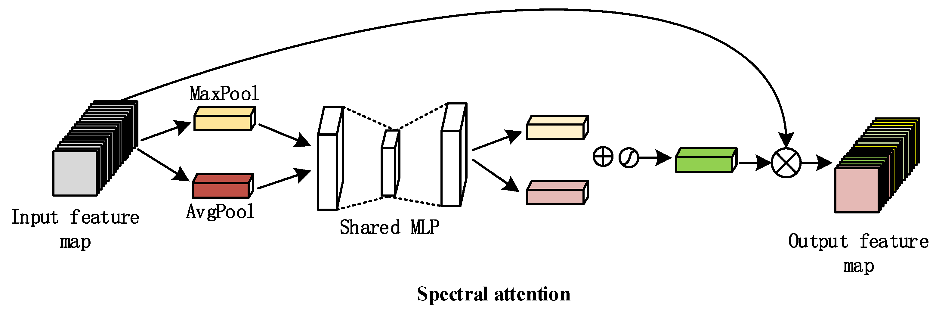
The attention mechanism [52] imitates the internal process of a biological observation behavior. It is a mechanism that aligns internal experience and external sensation to increase the observation precision and can quickly extract important features of coefficient data. The attention mechanism is currently an important concept in neural networks widely used in several computer vision tasks [53]. In this paper, we introduce the spectral attention module to enhance the feature extraction ability of the proposed deep learning network. Given a feature map as input, we define a 1-D spectral attention map . The purpose of using spectral attention is to extract information features useful for HSI classification by changing the weight of spectral information, which can be defined as presented in Equation (1).
where , is at position (m, n), ⊗ represents the multiplication element, the output of spectral attention, and max(.)the maximum area. and represent the global average and maximum pooling, respectively. The first FC layer is used as a dimensionality reduction layer parameterized by W0, while the second FC layer is a dimensionality increasing layer parameterized by W1. refers to the ReLU activation function, and , , , W0, and W1 are shared weights. Finally, we multiply with the input to obtain .
The spectral attention module is presented in Figure 1, where we use global average and global maximum pooling to extract the spectral information of the image. The two different pooling schemes extract more abstract spectral features, which are then followed by two FC layers and activation functions to establish two-pooling channel information. Then, we perform a correlation process to combine the weights of the two spectral feature channels. Finally, the newly assigned feature weight is multiplied by the input feature map to correct the weights of the input feature map and afford to extract higher-level feature information.
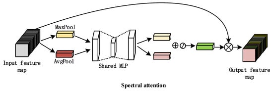
Figure 1.
Spectral attention mechanism. The module uses operations such as maximum pooling, average pooling, and shared weights to re-output feature maps with different weights.
2.2. Multi-Head Self-Attention
A CNN scheme is strictly limited by its kernel size and number of layers, thus weakening its advantage in capturing the long-range dependence of input data [52] and ultimately it is imposed to ignore some sequence information of the HSI input data. The self-attention mechanism improves the attention mechanism, which reduces the dependence on external information and can better capture the internal data correlation or its characteristic information. In this work, we utilize a self-attention variant to extract image features, namely the multi-head self-attention module.
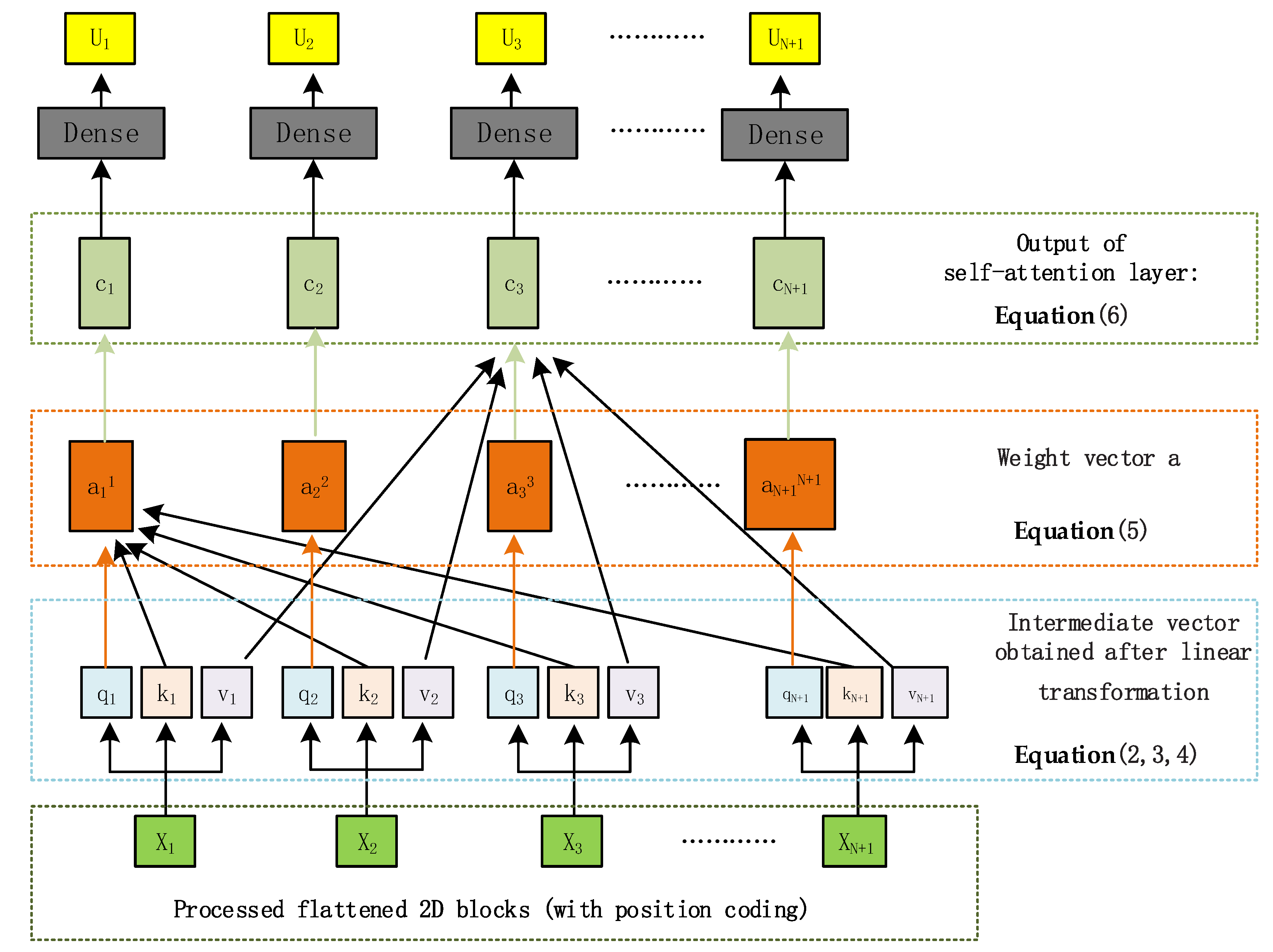
Therefore, we initially remap to , , by utilizing the three initialization transformation matrices , , and :
where is that the original HSI data is processed first, and then the block is noticed through the spectrum. The resulting flat 2D block with the same size , , and are three different weight matrices, which linearly change the input original vector and perform on each input three different linear transformations to obtain the intermediate vectors , , and , and ultimately increase the diversity of the model feature sampling.
Then, we calculate the weight vector according to the and parameters obtained from Equations (2) and (3), respectively, which is expressed as:
where , with N the number of flattened 2D blocks (Section 2.3 presents a detailed calculation of N). After that, we apply the dot product operation on the and , and divide by , where d is the dimensions of q and , respectively, to normalize the data. Finally, the weight vector is output through a softmax function. The vector depends on the vector and all vectors, and thus ultimately, Equation (5) produces in total N + 1 vectors with a length of N + 1 per vector.
Next, we combine Equations (4) and (5) to obtain the , and vector and perform a weighted average operation to calculate vector :
The output vector of Equation (6) is the weighted average of all vectors, with the weights provided by the vector.
Our deep learning pipeline combines a multi-head self-attention block under multiple self-attention concatenation schemes with the detailed process presented in Figure 2. The multi-head self-attention input is the vector produced by Equation (6), employing different , , and parameters during the matrix operations in Equations (2)–(4) to obtain different vectors. Ultimately, all outputs are stacked, forming the multi-head self-attention output. Finally, the latter output passes through a fully connected layer to create N + 1 u-vectors, where each vector has a one-to-one correspondence with .
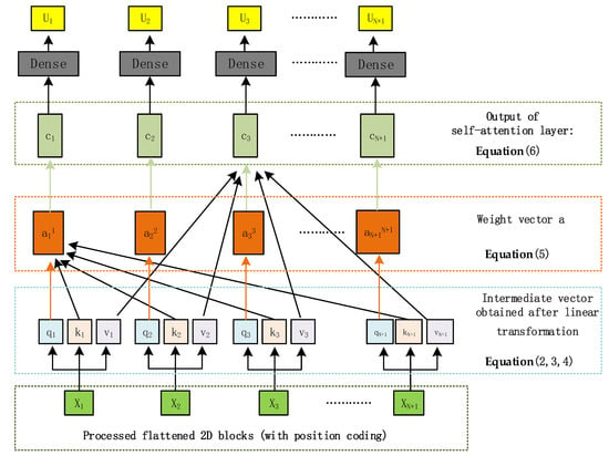
Figure 2.
Multi-Head Self-Attention structure: After mapping, linear change, matrix operation, and other operations, the output sequence obtained has the same length as the input sequence, and each output vector depends on all input vectors.
2.3. Encoder Block
According to the transformer concept employed in NLP and the suggestion of Dosovitskiy et al. [54], an image can be remapped into a sequence of flattened 2D patches . We extend [54] and add a processing step where the patch image obtained from the original data is mapped through the spectral attention block to extract the relevant features. Thus, ultimately, we obtain N flattened 2D blocks of the same size, with the dimension of each block being , with P the size of the setting block, , and H, W, C are the width, height, and channel number of the image, respectively. Then, for each vector, we perform a linear transformation (fully connected layer) and compress the dimension into dimension D. As a reference, we use the encoder model of the transformer, and since the decoder model is not used, we add a learnable embedding vector and introduce a positional encoding . This process is represented by:
where E represents the linear transformation layer, is the input dimension, and D is the output dimension. The trainable variable is used to represent the position information of the added sequence. When the positions are close, they often have similar codes, and the patches in the same line/column also have similar position codes.
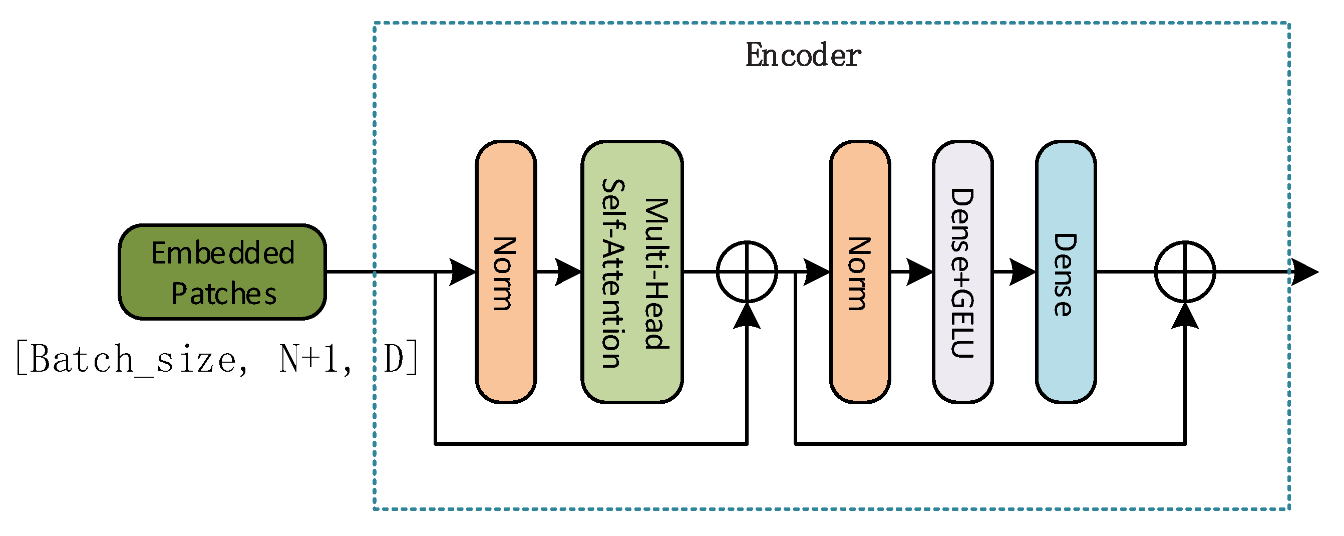
We design the encoder block by utilizing several operations, including the norm, multi-head self-attention, and dense, as expressed in Equation (8) and illustrated in Figure 3. It is worth noting that in the latter figure, the Gaussian Error Linear Unit (GELU) [55] activation function introduces the idea of random regularization, affording the network to converge faster and increasing the model’s generalization ability. Additionally, we employ multiple residual blocks to eliminate problems such as gradient dispersion. The Multilayer Perceptron (MLP) exploited contains two layers with a GELU non-linearity scheme. Finally, depending on the scenario, the encoder block presented in Figure 3 can be stacked multiple times as required to achieve a high HSI classification. The latter is discussed in Section 3.3, where LN represents Layer Normalization and MHSA multi-head Self-Attention.
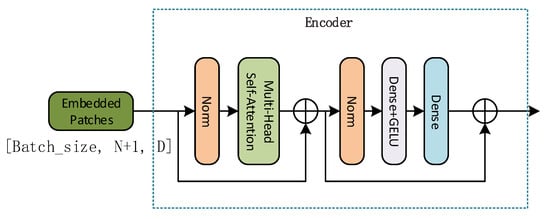
Figure 3.
Transformer Encoder Block. This module is composed of the norm, multi-head self-attention, and dense and other structures connected in the form of residuals.
2.4. Overview of the Proposed Model
Finally, the vectors obtained through stacked encoder modules are input to two fully connected layers employing GELU activation functions. Then, we exploit the first of the two vectors, i.e., the learnable embedding vector of the classification, to obtain the final classification result, which is expressed as:
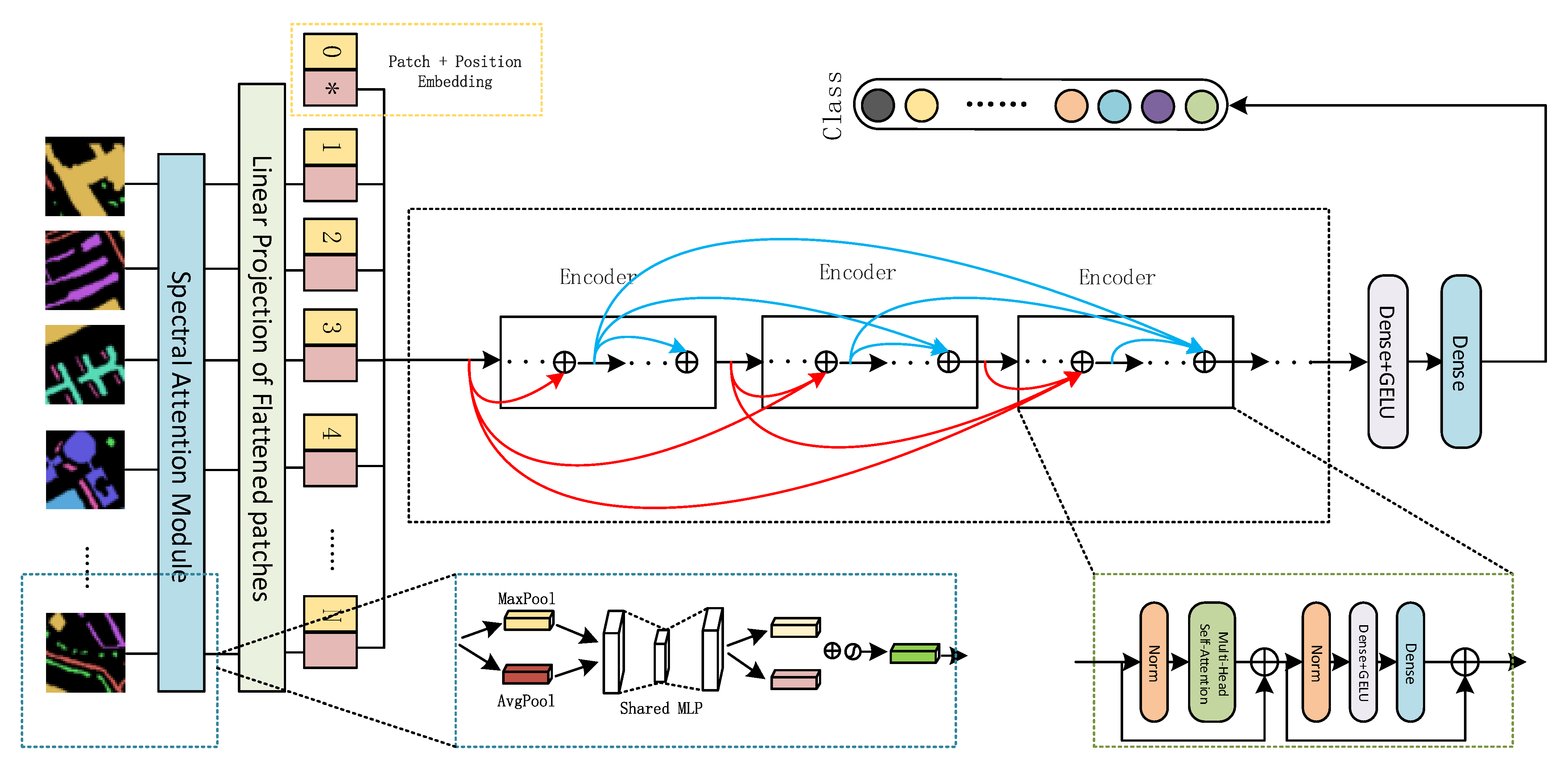
where is an additional embeddable vector used for classification and refers to the output of the encoder block, i.e., utilizing the dense, GELU, and dense blocks presented in Figure 4. The execution process of the entire SAT network is shown in the latter figure.
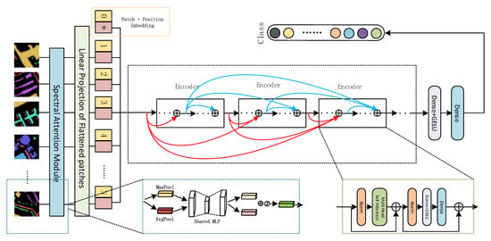
Figure 4.
The proposed SAT Net architecture. After the original HSI data is processed, it is input into the spectral attention and decoder modules with multi-head self-attention to extract HSI features. Second, the encoder module uses a multi-layer residual structure for connection, thereby effectively reducing information loss, and finally through the fully connected layer, it outputs classification information.
First, around each pixel, we extract patches of block size , with the third dimension being the spectral dimension of different his, while for the edge pixels that cannot be directly extracted, we employ a padding operation. Ultimately, we obtain the final sample data with shape , where m is the number of samples and is the width and height of the sample, respectively. A detailed analysis of the sample size is presented in Section 3.3. For the processed sample data, we pass it through the spectral attention module to redistribute the weight of the spectral information. Since the spectral attention mechanism does not change the shape of the input feature map, the shape of the output sample data is still .
Once the raw HSI data are remapped into a set of ( ) image patches, we process each sample into an sequence of flattened 2D patches with shape (P, P, o). However, the transformer-model expects a two-dimensional NxD matrix as an input (Remove the Batch_size dimension), where is the sequence length and D the dimension of each vector of the sequence (Set to 64 in this article). Therefore, we reshape the 2D patches into a two-dimensional matrix of shape (, o × P × P), and apply a linear transformation layer on the latter two-dimensional matrices to ultimately create a two-dimensional Matrix (N, D). Then, we introduce the embedding vector and the position code (as described in Section 2.2) and create a matrix of size (Batch_size, N + 1, D) (Add Batch_size dimension) used as the input to the encoder block. Here, we use multiple encoder modules (the specific number of modules is discussed in Section 3.3.3) to continue extracting image features. In contrast to Dosovitskiy et al. [54], we change the direct connection of a single encoder module and employ the residual structure to inter-connect each encoder module, with the detailed process shown in Figure 4. This strategy affords to reduce the information loss caused by stacking multiple encoder modules, and the model convergence speed is accelerated. The classification results are finally output through two fully connected layers.
3. Experiments, Results, and Discussion
In this section, we first introduce three publicly available HSI data sets and then analyze the five factors that influence the classification accuracy of the proposed model. Finally, we challenge the proposed model against current state-of-the-art methods and discuss the experimental results.
3.1. Data Set Description
For our experiments, we consider three publicly available HSI data sets, namely the Salinas (SA), the Indian Pines (IN), and the University of Pavia (UP). Detailed information on all datasets is presented in Table 1.

Table 1.
Datasets Employed During Trials.
3.1.1. Salinas (SA)
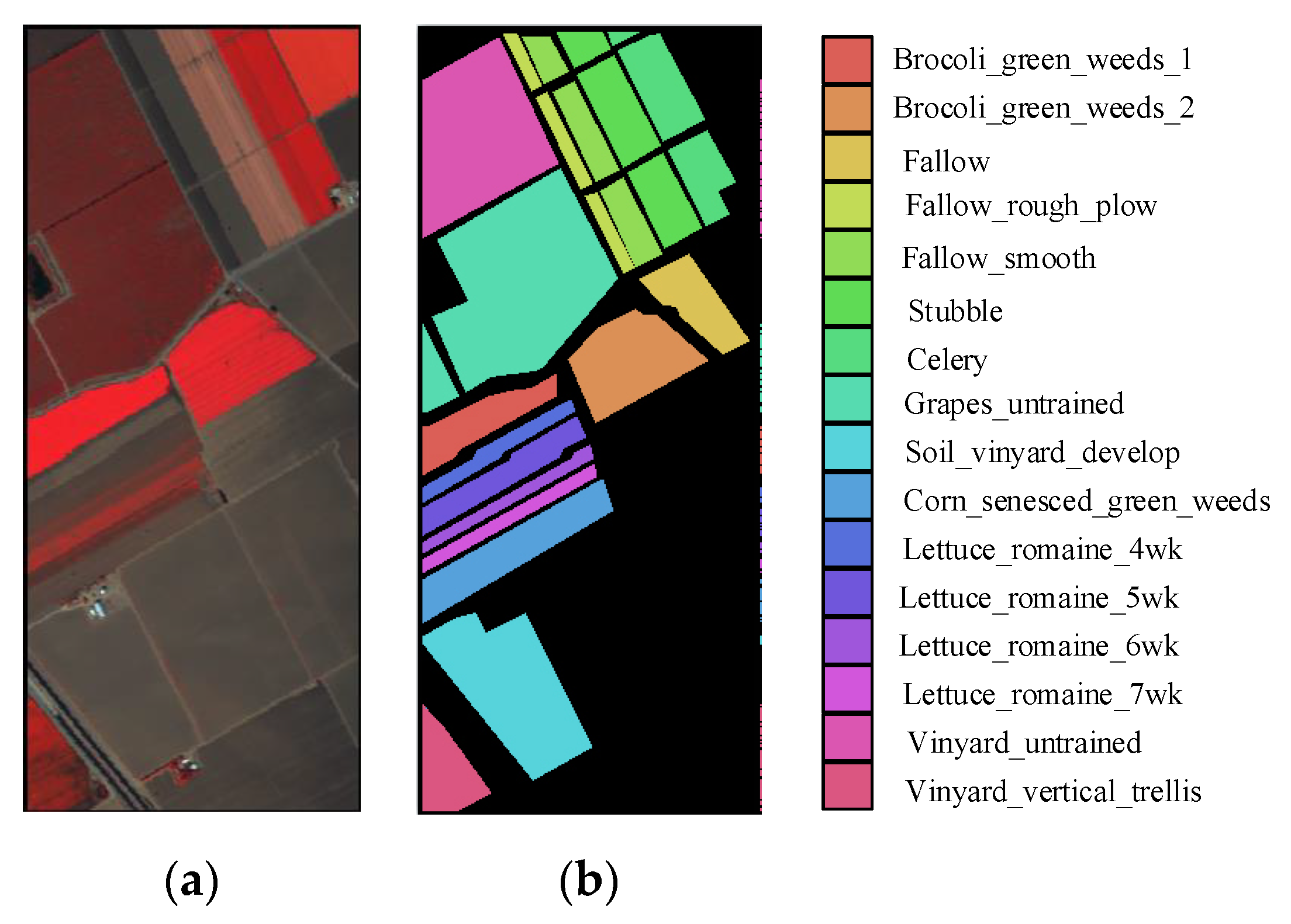
This dataset includes HSI collected by the Airborne Visible/Infrared Imaging Spectrometer (AVIRIS) sensor in Salinas, California, USA. It has 224 spectral bands and a spectral resolution of 400~2500 nm. Each HSI has a size of 512 × 217 pixels and a spatial resolution of 3.7 m/pixel. This dataset has in total 54,129 marked pixels presenting 16 object classes. The pseudo-color image and the corresponding ground truth map are illustrated in Figure 5, with the sample division ratio of the training and the test set shown in Table 2.
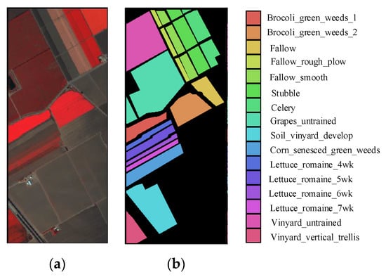
Figure 5.
Salinas images: (a) pseudo-color image; (b) ground-truth labels.

Table 2.
Training and Testing Samples for the SA Dataset.
3.1.2. Indian Pines (IN)
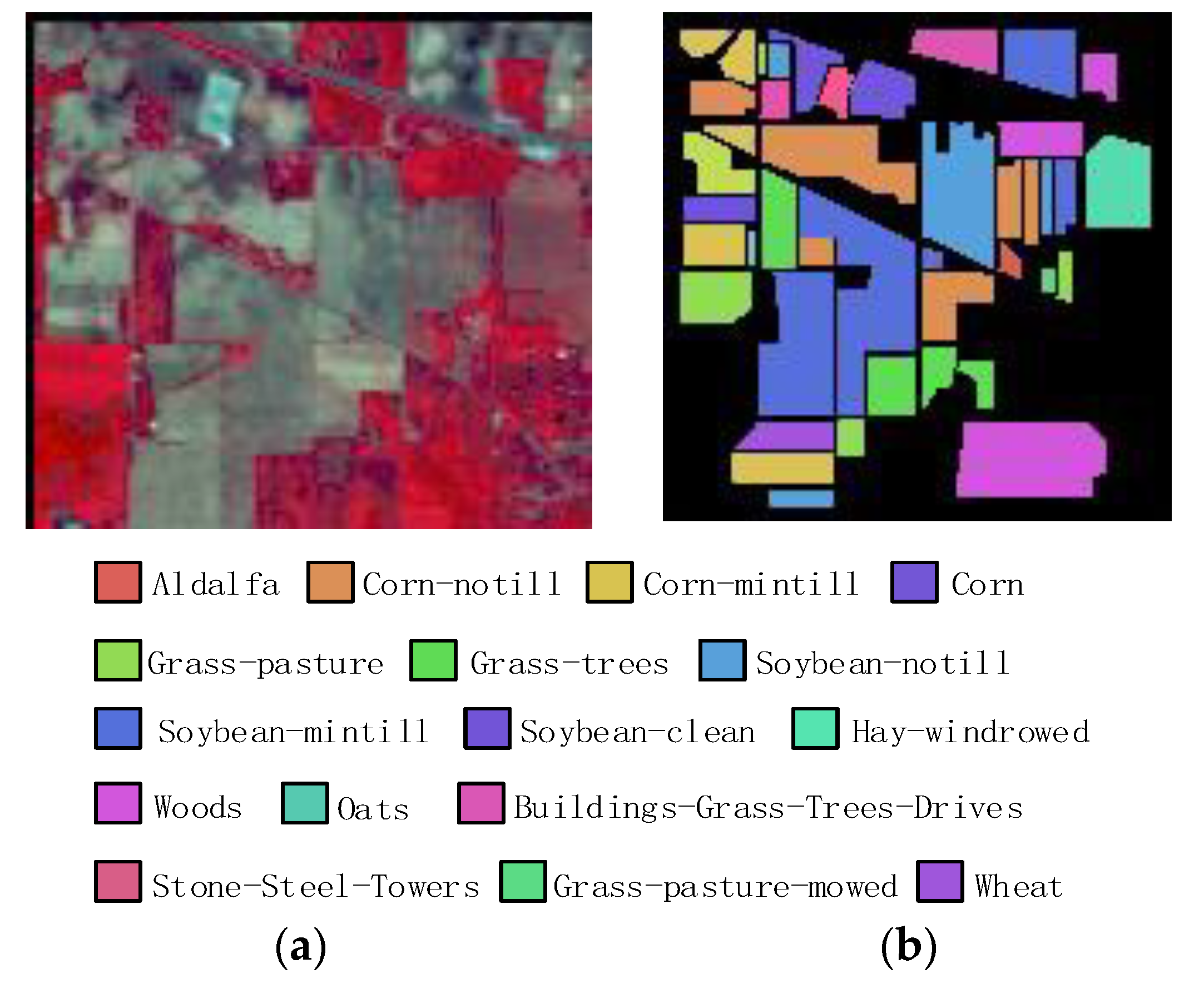
This dataset was collected by the AVIRIS sensor in Northwestern Indiana, USA involving 200 spectral bands and a spectral resolution of 400~2500 nm. It includes an HSI of 145 × 145 pixels and a spatial resolution of 20 m/pixel, with 10,249 marked pixels involving 16 object classes. The pseudo-color image and ground truth map are presented in Figure 6. The sample ratio between the training and the test set is shown in Table 3.
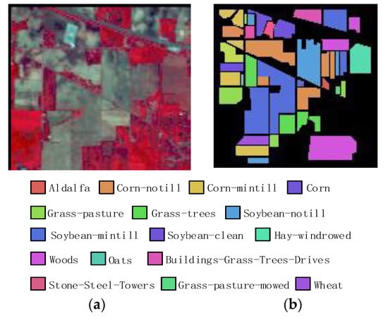
Figure 6.
Indian Pines images: (a) pseudo-color image; (b) ground-truth labels.

Table 3.
Training and Testing Samples for the IN Dataset.
3.1.3. University of Pavia (UP)
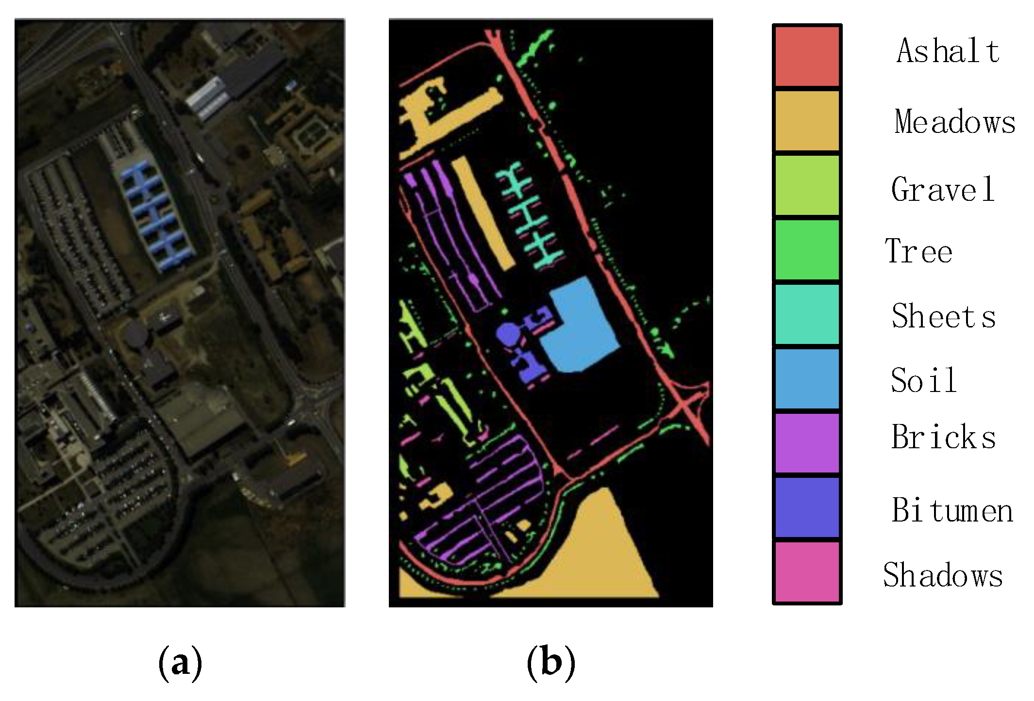
The Reflective Optics Spectrographic Imaging System (ROSIS) sensors collected this HSI in Pavia, Italy, involving imagery of 610 × 340 pixels and a spatial resolution of 1.3 m/pixel. The spectral bands are 103 with a resolution of 430~860 nm. In total, there are 42,776 marked pixels of nine object classes. The pseudo-color image and ground truth map are shown in Figure 7, with the training and test sets presented in Table 4.

Figure 7.
University of Pavia images: (a) pseudo-color image; (b) ground-truth labels.

Table 4.
Training and Testing Samples for the UP Dataset.
We randomly selected 20% of the dataset for training for our experiments, and the remaining 80% was for testing. A detailed experimental analysis is presented in Section 3.2.
3.2. Experimental Setup
We evaluate the performance of the proposed SAT Net model on an Intel(®) Xeon(®) Gold 5218 with 512 GB RAM and an NVIDIA(Headquartered in Santa Clara, CA, USA) Ampere A100 GPU with 40 GB RAM. Our platform operates on windows 10 utilizing the tensorflow2.2 deep learning framework and the python3.7 compiler. We optimize the model by exploiting the Adam optimizer [56] with a batch size of 64 and employ the cross-entropy loss function for reverse gradient propagation. We also employ a five-folder cross-validation [57] scheme to train and test the model in the experiments 3.3.1 and 3.3.2. Specifically: we divide each data set into five parts, accounting for 20% of the total data set. During each training round four parts are used as the training set and one part is used as the test set. In total, we consider five rounds of training exploiting each time a different subset of the data set as a training and a testing set. Finally, the average performance of the five test results is considered the model’s accuracy. In the experiments that follow. We quantitatively evaluate the performance of all competitor methods relying on the overall classification accuracy (OA), the average accuracy (AA), and the kappa coefficient (K).
3.3. Image Preprocessing
The first batch of trials involves investigating the interplay between the hyperparameter setup and the overall classification performance of the proposed SAT Net. These hyperparameters involve the extracted cube size, i.e., are the size of the 3D extracted patch, the size of the 2D patches, the number of stacked encoder blocks, the learning rate, and the proportion of training to testing samples.
3.3.1. Image Size (IS)
In this trial, we investigate the cube sizes of 16, 32, and 64, which are extracted around each pixel of the HSI raw data, with the corresponding results presented in Table 5. From the latter table, we observe that for IS = 16, the SA, IN, and UP datasets manage an OA of 97.18%, 93.42%, and 96.45%, respectively. However, despite the OA metric being relatively high, it is still lower than the optimum performance attained when IS = 64. This is because a smaller extraction cube interferes with the spatial continuity, while as IS increases, the performance also increases, and ultimately IS = 64 achieves the highest classification results. It should be noted that due to our hardware, our trials are limited to a maximum of IS = 64.

Table 5.
Evaluation of several hyperparameters under five-folder cross-validation. (Highest Performance is in Boldface).
3.3.2. Patch Size (PS)
In this experiment, we vary the size of the flattened 2D patch sequence. The different PS evaluated are inversely proportional to the number of the linear embedding sequences that are input to the encoder block. Thus, we set PS to 4, 8, and 16 with the corresponding results presented in Table 5. From the latter table, we confirm the findings of Dosovitskiy et al. [54] that , and thus for our trials, it should be greater than 16. Hence, for our trials, we employ a trial-and-reject strategy and conclude that for our method manages an appealing performance, which we adopt for the trials to follow.
3.3.3. Depth Size
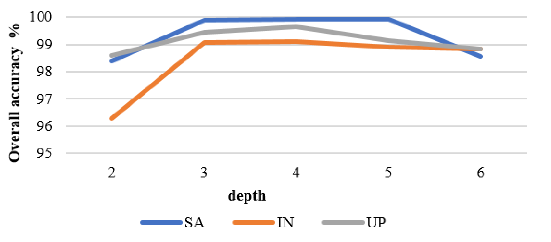
Here, we vary the number of stacked encoder blocks within the proposed SAT Net, with the stack cardinality set to 2, 3, 4, 5, and 6. The corresponding experimental results are shown in Figure 8, highlighting that as the number of encoder blocks increases, the classification accuracy increases, but also the total network parameters affecting the difficulty during network training increase as well. However, increasing the model parameters too much will cause the model to overfit and ultimately reduce its classification accuracy. For our trials, an encoder block cardinality of three manages a classification performance of 99.91%, 99.03%, and 99.47%, for the SA, IN, and UP datasets, respectively.
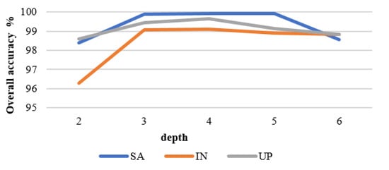
Figure 8.
Overall classification accuracy per dataset under various encoder block sizes.
3.3.4. Training Sample Ratio
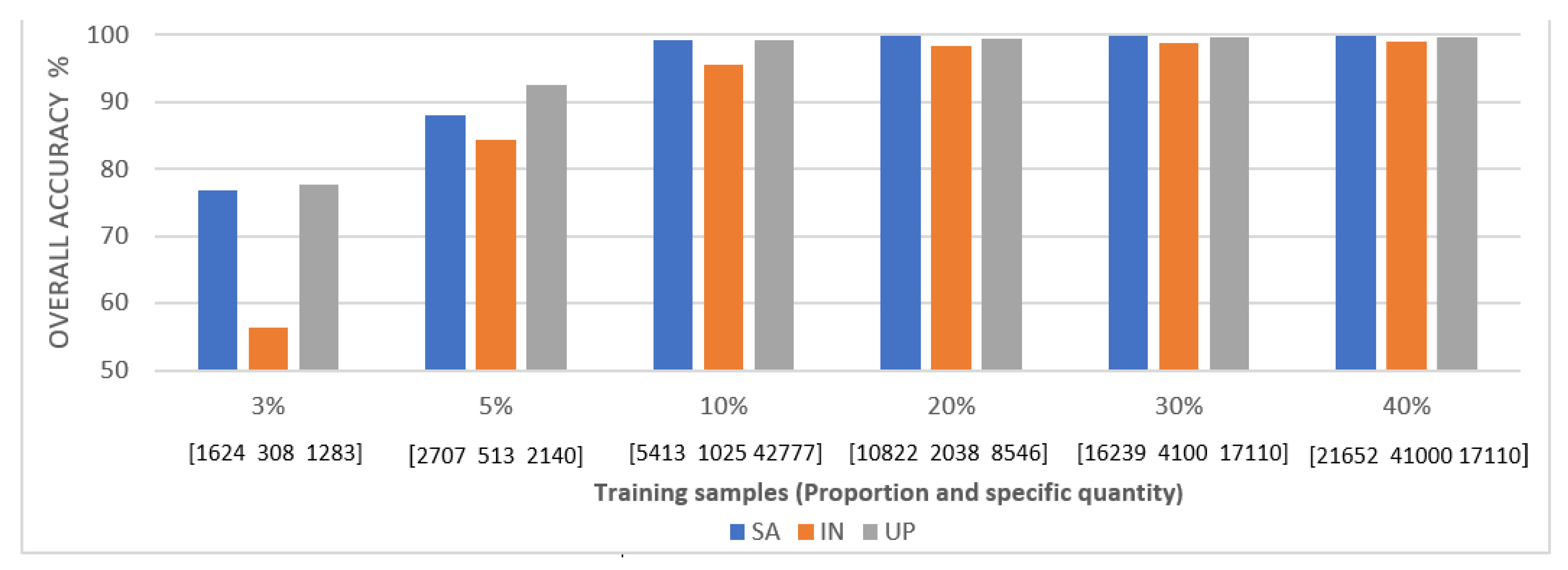
The proportion of training vs. testing data affects the fitting process of the model during its training. Hence, we evaluate the training proportions of 3%, 5%, 10%, 20%, 30%, and 40% of the entire dataset, with the corresponding results presented in Figure 9. From the latter figure, we observe that when the proportion of the training set is 3% and 5%, the classification result of IN is poor, and this is because the total number of samples in the IN dataset is relatively small. However, when the proportion of the training set exceeds 20%, all three datasets achieve quite appealing classification results. For the subsequent trials, and to compare our technique against current methods, e.g., Zhong et al. [25], we set the training set ratio to 20% of the total samples.

Figure 9.
Overall accuracy per dataset under different training set proportions.
3.3.5. Learning Rate
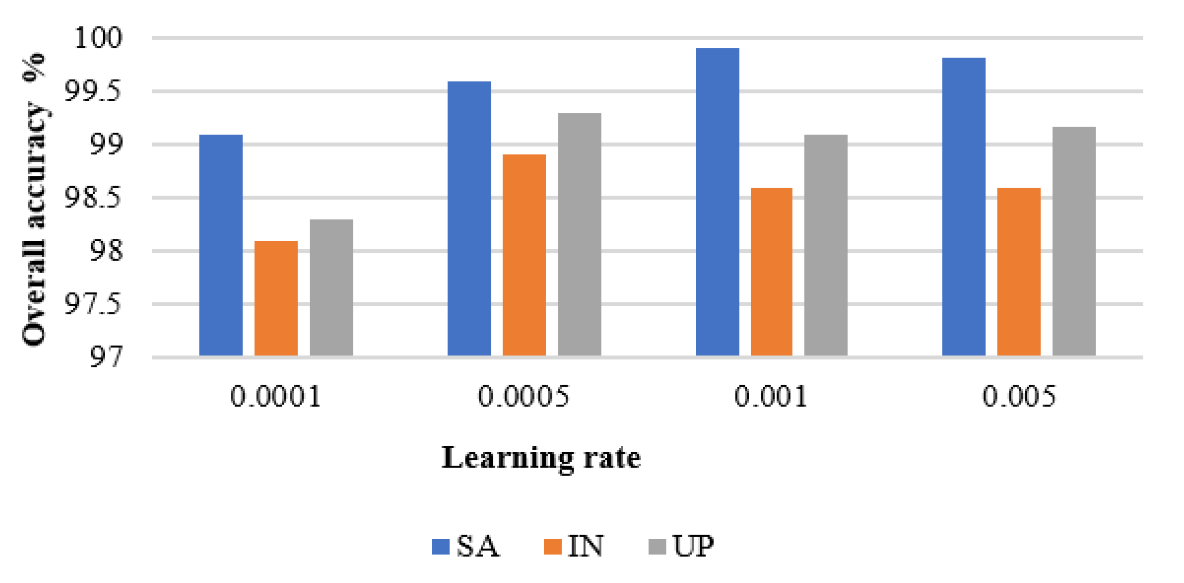
The learning rate affects the gradient descent rate of the model, and thus choosing an appropriate learning rate can control the convergence performance and speed of the model. For our experimental analysis, we set the learning rate to 0.0001, 0.0005, 0.001, and 0.005, respectively, with the corresponding results shown in Figure 10. We optimize SAT Net’s performance by setting the learning rate for SA to 0.001 and UP and IN to 0.0005.
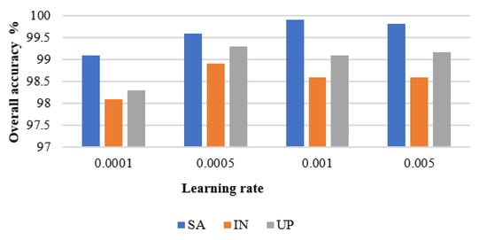
Figure 10.
The overall classification accuracy of the three data sets at different learning rates.
3.4. Evaluation
We challenge the proposed SAT Net against convolutional neural network (CNN) [58] (CNN architecture with five layers of weights), spectral attention module-based convolutional network (SA-MCN) [40] (Recalibrate spatial information and spectral information), three-dimensional convolutional neural network (3D-CNN) [32], and the spectral–spatial residual network (SSRN) [25], and the multi-scale residual network model with an attention mechanism (MSRN) [41]. For fairness, we set the ratio of training set and test set to 2:8. We also optimize the model by exploiting the Adam optimizer [56] with a batch size of 64 and employ the cross-entropy loss function for reverse gradient propagation.
3.4.1. Quantitative Evaluation
Table 6, Table 7 and Table 8 present the classification accuracy of each object class, and method evaluated exploiting the OA, AA, and K metrics. From the results, we observe that the CNN network, its classification results are still lacking due to the spectral feature information loss of the 2D-CNN that ignores the 3D nature of the HSI data. SA-MCN extracts spectral information features based on spectral attention. The 3D-CNN directly extracts the feature information of the spatial and spectral dimensions, which significantly improves the accuracy of HSI classification.

Table 6.
Classification Results of Various Methods for the SA Dataset (Highest Performance is in Boldface).

Table 7.
Classification Results of Various Methods for the IN Dataset (Highest Performance is in Boldface).

Table 8.
Classification Results of Various Methods for the UP Dataset (Highest Performance is in Boldface).
Nevertheless, 3D-CNN still does not fully utilize the space and spectrum-related information. On the contrary, SSRN exploits the spatial–spectrum attention module to redistribute the spatial and spectral information weights achieving good classification results. The proposed SAT Net attains the most appealing results over all three data sets, especially on the SA dataset, where it manages an overall classification accuracy of 99.91%. The MSRN network uses an improved residual network and space-spectral attention module to extract hyperspectral image information from different scales and multiple times, and fully integrates and extracts the spatial spectral features of the image. The best results are attained on the IN dataset managing an Overall accuracy, Average accuracy, and Kappa of 0.9937, 0.9945, and 0.9961, respectively. Regarding the proposed SAT Net, it obtains the most attractive results on the SA data set, as its overall classification accuracy, average classification accuracy and Kappa reaches 0.9991, 0.9963 and 0.9978, respectively. Finally, on the UP data set the proposed methods has comparable performance to MSRN. Indeed, the overall accuracy and Kappa coefficient are slightly inferior to the MSRN model, while the average accuracy is slightly superior to the MSRN model. Compared to the competitor methods, we extract the image features via a multi-head self-attention scheme that avoids partial information loss when utilizing regular convolution kernels during feature extraction and solves the problem of HSI long-distance dependence.
3.4.2. Qualitative Evaluation
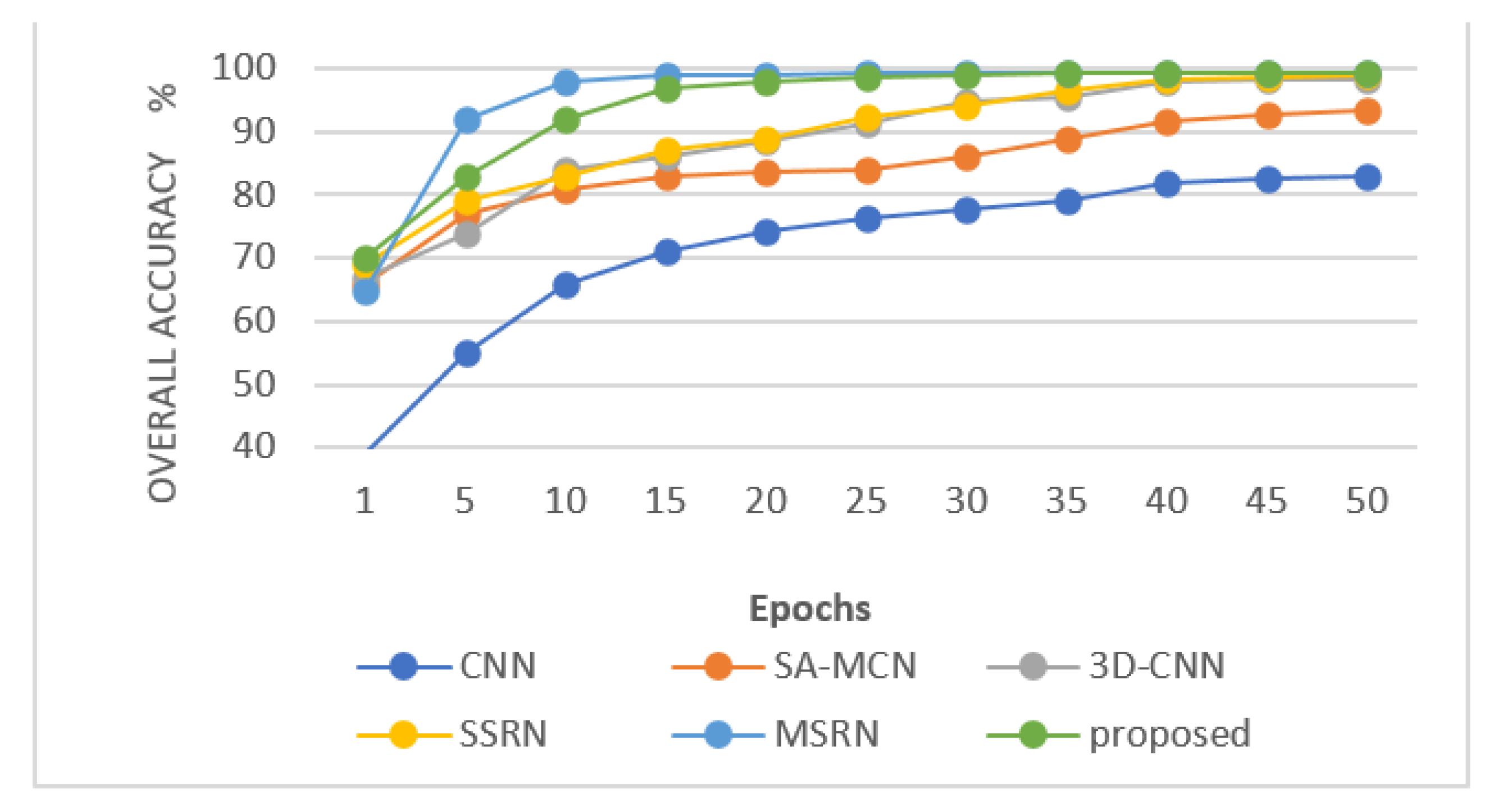
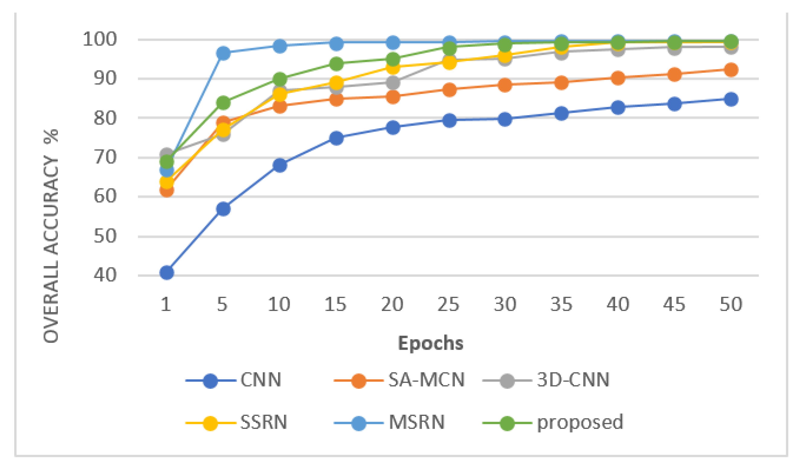
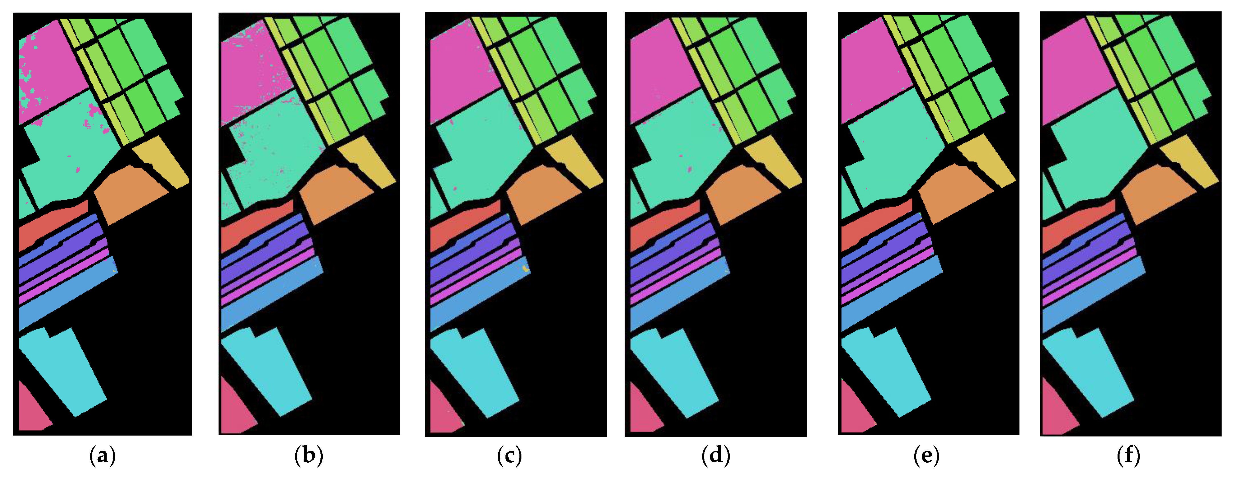
Figure 11, Figure 12 and Figure 13 show the overall accuracy curve of the proposed model against the competitor models. The results indicate that as the number of training steps increases, the accuracy of all models is continuously improving. Among the models, CNN has the lowest initial OA. SA-NET has the slowest convergence speed, MSRN has the fastest convergence speed, and SAT NET has the second-best convergence speed. The proposed model converges well in 20 epochs on the SA dataset and converges well within 30 epochs on the IN and UP datasets. Figure 14, Figure 15 and Figure 16 show the visualization results (pseudo-color classification map) of different models on the three public datasets we utilize in this work. The corresponding classification maps obtained by CNN, and SA-MCN manage an inferior performance, with significant noise levels, spectra, and poor continuity between different object classes. The results obtained by the 3D-CNN and SSRN methods are better, containing less point noise. MSRN also achieved good classification results. In contrast, the classification map generated by the proposed SAT Net model and MSRN has smoother boundaries, less noise, and overall manages a higher classification accuracy. Figure 17 is a partially enlarged view of the classification results of MSRN and SAT NET on the three datasets of SA, IN, and UP. It is observed from the enlarged image that in the SA dataset, the classification result of the SAT Net model has less continuous noise, and there is less noise only at the boundary between Grapes_untrained and Vinyard_untrained. In the IN dataset, MSRN and SAT Net have some pixel misdivisions at the border of Soybeans-clean till and Soybeans-min till. In the UP dataset, MSRN and SAT Net are mixed with some Meadow features in the bare soil features.
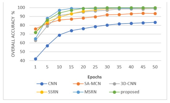
Figure 11.
Overall accuracy curve of different models in SA dataset.

Figure 12.
Overall accuracy curve of different models in IN dataset.
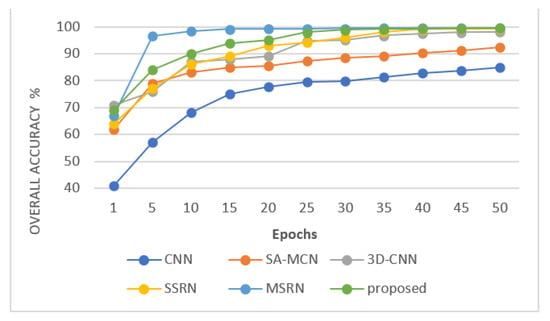
Figure 13.
Overall accuracy curve of different models in UP dataset.
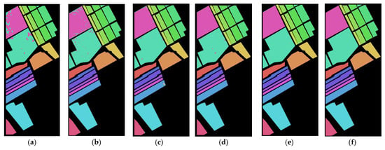
Figure 14.
The classification map on the SA dataset for (a) CNN, (b) SA-MCN, (c) 3D-CNN (d) SSRN, (e) MSRN, and (f) proposed SAT Net.

Figure 15.
The classification map on the IN dataset for (a) CNN, (b) SA-MCN, (c) 3D-CNN (d) SSRN, (e) MSRN, and (f) proposed SAT Net.

Figure 16.
The classification map on the UP dataset for (a) CNN, (b) SA-MCN, (c) 3D-CNN (d) SSRN, (e) MSRN, and (f) proposed SAT Net.

Figure 17.
(a) (MSRN) and (b) (SAT NET) are partial results of the UP dataset, (c) (MSRN), and (d) (SAT NET) are partial results of the UP dataset, (e) (MSRN) and (f) (SAT NET) are partial results of the UP dataset.
4. Conclusions
This article proposes a deep learning model that is appropriate for HSI classification entitled SAT Net. Our technique successfully employs a transformer scheme for HSI processing and proposes a new strategy for HSI image classification. Indeed, we first process the HSI data into a linear embedding sequence and then use the spectral attention module and the “multi-head self-attention” module to extract image features. The latter module solves long-distance dependence on the HSI spectral band and simultaneously discards the convolution operation avoiding information loss caused by the irregular processing of the typical convolution kernel during object classification. Overall, SAT Net combines multi-head self-attention and linear mapping, regularization, activation functions, and other operations to form an encoder block with a residual structure. To improve the performance of SAT Net, we stack multiple encoder blocks to form the main structure of our model. We verified the effectiveness of the proposed model by conducting two experiments on three publicly available datasets. The first experiment analyzes the interplay of our model’s hyperparameters, such as image size, training set ratio, and learning rate, to the overall attained classification performance. The second experiment challenges the proposed model against current classification methods. In comparison with models such as CNN, SA-MCN, 3D-CNN, and SSRN on the three public datasets, SAT NET’s OA, AA, and Kappa achieved better results. In comparison with MSRN, SAT NET achieved better results on the SA dataset. It achieved classification performance comparable to that of MSRN on the UP dataset, whereas it is slightly inferior to MSRN on the IN dataset; however, it uses less convolution (spectral attention module) to achieve better classification performance. In comparison with other methods, it provides a novel idea for HSI classification. Second, SAT NET better handles the long-distance dependence of HSI data spectrum information. On the three public data sets, i.e., SA, IN and UP, the proposed method achieved an overall accuracy of 99.91%, 99.22%, and 99.64% and an average accuracy of 99.63%, 99.08%, and 99.67%, respectively. Due to the small number of samples in the IN data set and the uneven data distribution, the classification performance of the SAT network still needs to be improved. In the future, we will study methods such as data expansion, weighted loss function, and model optimization to improve the classification of small-sampled hyperspectral data.
Author Contributions
Conceptualization, Y.Q. and W.L.; methodology, Y.Q. and W.L.; software, Y.Q. and W.L.; validation, Y.Q., L.F. and W.G.; formal analysis, Y.Q., L.F. and W.G.; writing—original draft preparation, Y.Q., W.L. and L.F.; writing—review and editing, Y.Q. and W.L.; visualization, Y.Q., W.L., L.F. and W.G. All authors have read and agreed to the published version of the manuscript.
Funding
This research received no external funding.
Conflicts of Interest
The authors declare no conflict of interest.
References
- Ghiyamat, A.; Shafri, H.Z. A review on hyperspectral remote sensing for homogeneous and heterogeneous forest biodiversity assessment. Int. J. Remote Sens. 2010, 31, 1837–1856. [Google Scholar] [CrossRef]
- Fauvel, M.; Tarabalka, Y.; Benediktsson, J.A.; Chanussot, J.; Tilton, J.C. Advances in spectral-spatial classification of hyperspectral images. Proc. IEEE 2013, 101, 652–675. [Google Scholar] [CrossRef]
- Li, W.; Du, Q. Joint within-class collaborative representation for hyperspectral image classification. IEEE J. Sel. Top. Appl. Earth Obs. Remote Sens. 2014, 7, 2200–2208. [Google Scholar] [CrossRef]
- Manjunath, K.; Ray, S.; Vyas, D. Identification of indices for accurate estimation of anthocyanin and carotenoids in different species of flowers using hyperspectral data. Remote Sens. Lett. 2016, 7, 1004–1013. [Google Scholar] [CrossRef]
- Zhang, X.; Sun, Y.; Shang, K.; Zhang, L.; Wang, S. Crop classification based on feature band set construction and object-oriented approach using hyperspectral images. IEEE J. Sel. Top. Appl. Earth Observ. Remote Sens. 2016, 9, 4117–4128. [Google Scholar] [CrossRef]
- Zheng, X.; Yuan, Y.; Lu, X. Dimensionality reduction by spatial–spectral preservation in selected bands. IEEE Trans. Geosci. Remote Sens. 2017, 55, 5185–5197. [Google Scholar] [CrossRef]
- He, L.; Li, J.; Liu, C.; Li, S. Recent advances on spectral–spatial hyperspectral image classification: An overview and new guidelines. IEEE Trans. Geosci. Remote Sens. 2018, 56, 1579–1597. [Google Scholar] [CrossRef]
- Khan, M.J.; Khan, H.S.; Yousaf, A.; Khurshid, K.; Abbas, A. Modern trends in hyperspectral image analysis: A review. IEEE Access 2018, 6, 14118–14129. [Google Scholar] [CrossRef]
- Luo, F.; Du, B.; Zhang, L.; Zhang, L.; Tao, D. Feature learning using spatial–spectral Hypergraph discriminant analysis for hyperspectral image. IEEE Trans. Cybern. 2019, 49, 2406–2419. [Google Scholar] [CrossRef]
- Paoletti, M.E.; Haut, J.M.; Fernandez-Beltran, R.; Plaza, J.; Plaza, A.; Li, J.; Pla, F. Capsule networks for hyperspectral image classification. IEEE Trans. Geosci. Remote Sens. 2019, 57, 2145–2160. [Google Scholar] [CrossRef]
- Kang, X.; Li, S.; Benediktsson, J.A. Spectral–spatial hyperspectral image classification with edge-preserving filtrering. IEEE Trans. Geosci. Remote Sens. 2014, 52, 2666–2677. [Google Scholar] [CrossRef]
- Liu, J.; Wu, Z.; Wei, Z.; Xiao, L.; Sun, L. Spatial-spectral kernel sparse representation for hyperspectral image classification. IEEE J. Sel. Top. Appl. Earth Obs. Remote Sens. 2013, 6, 2462–2471. [Google Scholar] [CrossRef]
- Chi, M.; Feng, R.; Bruzzone, L. Classification of hyperspectral remote-sensing data with primal SVM for small-sized training dataset problem. Adv. Space Res. 2008, 41, 1793–1799. [Google Scholar] [CrossRef]
- Haut, J.; Paoletti, M.; Plaza, J.; Plaza, A. Cloud implementation of the K-means algorithm for hyperspectral image analysis. J. Supercomput. 2017, 73, 514–529. [Google Scholar] [CrossRef]
- Tarabalka, Y.; Fauvel, M.; Chanussot, J.; Benediktsson, J.A. SVMand MRF-based method for accurate classification of hyperspectral images. IEEE Geosci. Remote Sens. Lett. 2010, 7, 736–740. [Google Scholar] [CrossRef]
- Kang, J.; Hong, D.; Liu, J.; Baier, G.; Yokoya, N.; Demir, B. Learning convolutional sparse coding on complex domain for interferometric phase restoration. IEEE Trans. Neural Netw. Learn. Syst. 2021, 32(2), 826–840. [Google Scholar] [CrossRef] [PubMed]
- LeCun, Y.; Bengio, Y.; Hinton, G. Deep learning. Nature 2015, 521, 436–444. [Google Scholar] [CrossRef]
- Lu, X.; Wang, B.; Zheng, X.; Li, X. Exploring models and data for remote sensing image caption generation. IEEE Trans. Geosci. Remote Sens. 2018, 56, 2183–2195. [Google Scholar] [CrossRef]
- Deng, C.; Xue, Y.; Liu, X.; Li, C.; Tao, D. Active transfer learning network: A unified deep joint spectral–spatial feature learning model for hyperspectral image classification. IEEE Trans. Geosci. Remote Sens. 2019, 57, 1741–1754. [Google Scholar] [CrossRef]
- Zhao, C.; Wan, X.; Zhao, G.; Cui, B.; Liu, W.; Qi, B. Spectralspatial classification of hyperspectral imagery based on stacked sparse autoencoder and random forest. Eur. J. Remote Sens. 2017, 50, 47–63. [Google Scholar] [CrossRef]
- Zhou, S.; Xue, Z.; Du, P. Semisupervised stacked autoencoder with cotraining for hyperspectral image classification. IEEE Trans. Geosci. Remote Sens. 2019, 57, 3813–3826. [Google Scholar] [CrossRef]
- Chen, Y.; Zhao, X.; Jia, X. Spectral–spatial classification of hyperspectral data based on deep belief network. IEEE J. Sel. Top. Appl. Earth Observ. Remote Sens. 2015, 8, 2381–2392. [Google Scholar] [CrossRef]
- Zhou, F.; Hang, R.; Liu, Q.; Yuan, X. Hyperspectral image classification using spectral-spatial LSTMs. Neurocomputing 2019, 328, 39–47. [Google Scholar] [CrossRef]
- Hang, R.; Liu, Q.; Hong, D.; Ghamisi, P. Cascaded recurrent neural networks for hyperspectral image classification. IEEE Trans. Geosci. Remote Sens. 2019, 57, 5384–5394. [Google Scholar] [CrossRef]
- Zhong, Z.; Li, J.; Luo, Z.; Chapman, M. Spectral–Spatial residual network for hyperspectral image classification: A 3-D deep learning framework. IEEE Trans. Geosci. Remote Sens. 2018, 56, 847–858. [Google Scholar] [CrossRef]
- Song, W.; Li, S.; Fang, L.; Lu, T. Hyperspectral image classification with deep feature fusion network. IEEE Trans. Geosci. Remote Sens. 2018, 56, 3173–3184. [Google Scholar] [CrossRef]
- Mei, S.; JI, J.; Bi, Q.; Hou, J.; Du, Q.; Li, W. Integrating spectral and spatial information into deep convolutional neural networks for hyperspectral classification. IEEE Int. Geosci. Remote Sens. Symp. 2016, 5067–5070. [Google Scholar]
- He, K.; Zhang, X.; Ren, S.; Sun, J. Deep residual learning for image recognition. In Proceedings of the IEEE Conference on Computer Vision and Pattern Recognition, Las Vegas, NV, USA, 27–30 June 2016; pp. 770–778. [Google Scholar]
- Wang, L.; Peng, J.; Sun, W. Spatial–Spectral Squeeze-and-Excitation Residual Network for Hyperspectral Image Classification. Remote Sens. 2019, 11, 884. [Google Scholar] [CrossRef]
- Paoletti, M.E.; Haut, J.M.; Fernandez-Beltran, R.; Plaza, J.; Plaza, A.J.; Pla, F. Deep pyramidal residual networks for spectral-spatial hyperspectral image classification. IEEE Trans. Geosci. Remote Sens. 2018. to be published. [Google Scholar] [CrossRef]
- Lee, H.; Kwon, H. Going deeper with contextual CNN for hyperspectral image classification. IEEE Trans. Image Process. 2017, 26, 4843–4855. [Google Scholar] [CrossRef]
- Chen, Y.; Jiang, H.; Li, C.; Jia, X.; Ghamisi, P. Deep feature extraction and classification of hyperspectral images based on convolutional neural networks. IEEE Trans. Geosci. Remote Sens. 2016, 54, 6232–6251. [Google Scholar] [CrossRef]
- Seydgar, M.; Alizadeh Naeini, A.; Zhang, M.; Li, W. 3-D convolution-recurrent networks for spectral-spatial classification of hyperspectral images. Remote Sens. 2019, 11, 833. [Google Scholar] [CrossRef]
- Rao, M.; Tang, P.; Zhang, Z. A Developed Siamese CNN with 3D Adaptive Spatial-Spectral Pyramid Pooling for Hyperspectral Image Classification. Remote Sens. 2020, 12, 1964. [Google Scholar] [CrossRef]
- Gao, F.; Huang, T.; Sun, J.; Wang, J.; Hussain, A.; Yang, E. A New Algorithm of SAR Image Target Recognition Based on Improved Deep Convolutional Neural Network. Cogn. Comput. 2019, 11, 809–824. [Google Scholar] [CrossRef]
- Zhu, M.; Jiao, L.; Liu, F.; Yang, S.; Wang, J. Residual Spectral–Spatial Attention Network for Hyperspectral Image Classification. IEEE Trans. Geosci. Remote Sens. 2021, 59, 449–462. [Google Scholar] [CrossRef]
- Haut, J.M.; Paoletti, M.E.; Plaza, J.; Plaza, A.; Li, J. Visual Attention-Driven Hyperspectral Image Classification. IEEE Trans. Geosci. Remote Sens. 2019, 57, 8065–8080. [Google Scholar] [CrossRef]
- Wu, P.; Cui, Z.; Gan, Z.; Liu, F. Residual Group Channel and Space Attention Network for Hyperspectral Image Classification. Remote Sens. 2020, 12, 2035. [Google Scholar] [CrossRef]
- Li, L.; Yin, J.; Jia, X.; Li, S.; Han, B. Joint Spatial-Spectral Attention Network for Hyperspectral Image Classification. IEEE Geosci. Remote Sens. Lett. 2020, 1–5. [Google Scholar] [CrossRef]
- Mou, L.; Zhu, X.X. Learning to pay attention on spectral domain: A spectral attention module-based convolutional network for hyperspectral image classification. IEEE Trans. Geosci. Remote Sens. 2020, 58, 110–122. [Google Scholar] [CrossRef]
- Qing, Y.; Liu, W. Hyperspectral Image Classification Based on Multi-Scale Residual Network with Attention Mechanism. Remote Sens. 2021, 13, 335. [Google Scholar] [CrossRef]
- Zhu, J.; Fang, L.; Ghamisi, P. Deformable Convolutional Neural Networks for Hyperspectral Image Classification. IEEE Geosci. Remote Sens. Lett. 2018, 15, 1254–1258. [Google Scholar] [CrossRef]
- Vaswani, A.; Shazeer, N.; Parmar, N.; Uszkoreit, J.; Jones, L.; Gomez, A.N.; Kaiser, L.; Polosukhin, I. Attention is all you need. arXiv 2017, arXiv:1706.03762v5. [Google Scholar]
- Devlin, J.; Chang, M.-W.; Lee, K.; Toutanova, K. Bert: Pretraining of deep bidirectional transformers for language understanding. arXiv 2018, arXiv:1810.04805. [Google Scholar]
- Brown, T.B.; Mann, B.; Ryder, N.; Subbiah, M.; Kaplan, J.; Dhariwal, P.; Neelakantan, A.; Shyam, P.; Sastry, G.; Askell, A.; et al. Language models are few-shot learners. arXiv 2020, arXiv:2005.14165. [Google Scholar]
- Radford, A.; Wu, J.; Child, R.; Luan, D.; Amodei, D.; Sutskever, I. Language models are unsupervised multitask learners. OpenAI Blog. 2019, 1, 9. [Google Scholar]
- Agrawal, A.; Jha, A.K.; Jaiswal, A.; Kumar, V. Irony Detection Using Transformers. In Proceedings of the International Conference on Computing and Data Science (CDS), Stanford, CA, USA, 1–2 August 2020; pp. 165–168. [Google Scholar] [CrossRef]
- Touvron, H.; Cord, M.; Douze, M.; Massa, F.; Sablayrolles, A.; Jegou, H. Training data-efficient image transformers & distillation through attention. arXiv 2020, arXiv:2012.12877. [Google Scholar]
- Carion, N.; Massa, F.; Synnaeve, G.; Usunier, N.; Kirillov, A.; Zagoruyko, S. End-to-end object detection with transformers. arXiv 2020, arXiv:2005.12872. [Google Scholar]
- Yang, F.; Yang, H.; Fu, J.; Lu, H.; Guo, B. Learning texture transformer network for image super-resolution. In Proceedings of the IEEE Conference on Computer Vision and Pattern Recognition (CVPR), Seattle, WA, USA, 13–19 June 2020; pp. 5791–5800. [Google Scholar]
- Girdhar, R.; Carreira, J.; Doersch, C.; Zisserman, A. Video action transformer network. In Proceedings of the IEEE Conference on Computer Vision and Pattern Recognition, Long Beach, CA, USA, 15–20 June 2019; pp. 244–253. [Google Scholar]
- Wang, F.; Tax, D.M. Survey on the attention based rnn model and its applications in computer vision. arXiv 2016, arXiv:1601.06823. [Google Scholar]
- Woo, S.; Park, J.; Lee, J.Y.; Kweon, I.S. CBAM: Convolutional Block Attention Module. In Computer Vision–ECCV 2018. ECCV 2018; Lecture Notes in Computer Science; Ferrari, V., Hebert, M., Sminchisescu, C., Weiss, Y., Eds.; Springer: Berlin, Germany, 2018; Volume 11211, pp. 3–19. [Google Scholar] [CrossRef]
- Dosovitskiy, A.; Beyer, L.; Kolesnikov, A. An Image is Worth 16x16 Words: Transformers for Image Recognition at Scale. arXiv 2020, arXiv:2010.11929. [Google Scholar]
- Hendrycks, D.; Gimpel, K. Gaussian Error Linear Units (GELUs). arXiv 2016, arXiv:1606.08415V3. [Google Scholar]
- Kingma, D.P.; Ba, J. Adam: A method for Stochastic Optimization. arXiv 2014, arXiv:1412.6980v8. [Google Scholar]
- Zhang, S.; Sun, F.; Wang, N.; Zhang, C.; Yu, Q.; Zhang, M.; Zhong, H. Computer-Aided Diagnosis (CAD) of Pulmonary Nodule of Thoracic CT Image Using Transfer Learning. J. Digit. Imaging 2019, 32, 995–1007. [Google Scholar] [CrossRef] [PubMed]
- Hu, W.; Huang, Y.; Wei, L.; Zhang, F.; Li, H. Deep convolutional neural networks for hyperspectral image classification. J. Sens. 2015, 2015, 12. [Google Scholar] [CrossRef]
Publisher’s Note: MDPI stays neutral with regard to jurisdictional claims in published maps and institutional affiliations. |
© 2021 by the authors. Licensee MDPI, Basel, Switzerland. This article is an open access article distributed under the terms and conditions of the Creative Commons Attribution (CC BY) license (https://creativecommons.org/licenses/by/4.0/).

