Abstract
Quantifying the mass balance of the Antarctic Ice Sheet (AIS), and the resulting sea level rise, requires an understanding of inter-annual variability and associated causal mechanisms. Very few studies have been exploring the influence of climate anomalies on the AIS and only a vague estimate of its impact is available. Changes to the ice sheet are quantified using observations from space-borne altimetry and gravimetry missions. We use data from Envisat (2002 to 2010) and Gravity Recovery And Climate Experiment (GRACE) (2002 to 2016) missions to estimate monthly elevation changes and mass changes, respectively. Similar estimates of the changes are made using weather variables (surface mass balance (SMB) and temperature) from a regional climate model (RACMO2.3p2) as inputs to a firn compaction (FC) model. Elevation changes estimated from different techniques are in good agreement with each other across the AIS especially in West Antarctica, Antarctic Peninsula, and along the coasts of East Antarctica. Inter-annual height change patterns are then extracted using for the first time an empirical mode decomposition followed by a principal component analysis to investigate for influences of climate anomalies on the AIS. Investigating the inter-annual signals in these regions revealed a sub-4-year periodic signal in the height change patterns. El Niño Southern Oscillation (ENSO) is a climate anomaly that alters, among other parameters, moisture transport, sea surface temperature, precipitation, in and around the AIS at similar frequency by alternating between warm and cold conditions. This periodic behavior in the height change patterns is altered in the Antarctic Pacific (AP) sector, possibly by the influence of multiple climate drivers, like the Amundsen Sea Low (ASL) and the Southern Annular Mode (SAM). Height change anomaly also appears to traverse eastwards from Coats Land to Pine Island Glacier (PIG) regions passing through Dronning Maud Land (DML) and Wilkes Land (WL) in 6 to 8 years. This is indicative of climate anomaly traversal due to the Antarctic Circumpolar Wave (ACW). Altogether, inter-annual variability in the SMB of the AIS is found to be modulated by multiple competing climate anomalies.
1. Introduction
The Antarctic ice sheet (AIS) is the largest reservoir of fresh water on Earth and has a potential to raise global sea level by 58 m in the worst case, which is if it were to melt completely [1]. Steig et al. (2009) have pointed towards a warming Antarctica since the late twentieth century [2]. Since then, observing the AIS has been a priority as it was found to be a primary contributor to global sea-level rise with high vulnerability [3]. Studies have shown that the AIS contributes nearly 0.60 mm year to the global mean sea level (GMSL) during 1993–2010 [4]. However, the contribution of the AIS is non uniform spatially and varies basin-to-basin at differing scales, leading to multiple mass redistribution patterns [5,6].
Antarctica is subject to climate driven fluctuations with inter-annual periods [7,8]. Among them, El Niño Southern Oscillation (ENSO) brings along anomalies in sea surface temperature (SST), sea ice extent, ice shelf thinning rates, and surface melt events in and around Antarctica [9,10,11]. ENSO also causes simultaneous high and low pressure systems leading to larger cloud formation and precipitation. This often leads to fluctuations in the normal mass change trends [12] and can influence the nominal mass change patterns in Antarctica [9,13]. Similar anomalies were detected in surface mass and elevation change estimated from space-borne geodetic techniques which had a periodicity of 4 to 6 years and circle the AIS in 9 to 10 years [14]. These anomalies may be attributed to ENSO contributions over the AIS or the Antarctic circumpolar wave (ACW), a large scale co-varying oceanic and atmospheric anomaly propagating eastward across the Southern Ocean (SO) on subdecadal time scales [15,16,17]. Yet, the inter-annual geodetic signal has not been corroborated by a climate model that could confirm an atmospheric origin.
Due to its large size and extreme climate conditions, more thorough understanding of the AIS has been possible only using remote sensing techniques. Indeed, remote sensing has emerged and evolved as a new observer of the AIS since the latter half of the twentieth century. Remote sensing missions primarily focused on studying the atmosphere and the oceans. The surface topography is also one of the key parameters that came into prominence later on [18]. Indeed, it acts as a factor between regional climate and the consequent response of an ice sheet both in short and long terms. Altimetry, either radar or laser, could monitor changes of the topography. Since the 1990s, the AIS has been closely monitored using satellite altimetry missions, such as ERS-1, ERS-2, Envisat, etc. [19,20]. Measurement of changes in surface elevation of the ice sheets is used to quantify volume changes and estimate mass changes. The mass change of the AIS is a paramount parameter to monitor the ice sheet equilibrium [21]. Since 2002, monitoring of the mass change is possible with the Gravity Recovery And Climate Experiment (GRACE) mission and since 2018, its successor, the GRACE-Follow On mission [22,23]. These two space-borne gravimetry missions could retrieve gravity changes that are partly due to surface-mass variations in Antarctica [24,25,26]. Global observations of water and ice mass redistribution in the Earth system at monthly to decadal time scales from GRACE missions played a critical role in understanding the climate system and investigating its changes [27]. Errors encountered and uncertainty associated while deriving mass changes from GRACE observations are already been taken into account comprehensively [28]. Thorvaldsen et al. [29] function as a necessary complete guide for products available for investigating climate change in the AIS. Apart from the constrained and limited space-borne observations, weather variables, like accumulation and temperature, are estimated from climate models, such as RACMO2.3p2, for Antarctica [30]. The development of such climate models is facilitated by the evolution of high computing performance together with the availability of long-term observations of the atmosphere.
Since we have continuous long-term observations of the AIS from three distinct techniques, it is imperative to have a combined analysis using each of them. As Gao et al. (2019) [31] suggest, combined analysis using multiple data sets give better estimates rather than from a single technique or data set. Multiple studies talk about the influence of climate processes and presence of climate process signature in the ice sheet mass balance at multiple scales [9,12,13,14] but have not explored it based on mass balance estimates from a climate model to establish a possible climate origin. A recent study using surface mass balance estimates and GRACE data by Zhang et al. (2021) [32] finds correlation between inter-annual ice mass variations on a regional scale and ENSO index. Therefore, we make three independent estimate of changes and investigate the inter-annual variability of these estimates by successively applying for the first time an Empirical Mode Decomposition and a Principal Component Analysis. We characterize these inter-annual signals and investigate for possible signatures associated with climate driven changes locally. We first introduce the data sets we use in Section 2 and explain how we derived height changes in Section 3. In Section 4, we present our methodology to extract inter-annual signals in Antarctica and discuss our results in Section 5. Our conclusions are summarized in Section 6.
2. Data
We rely on space-based geodetic observations and a climate model to study surface changes of the AIS.
2.1. Altimetry Data
The AIS has been closely monitored using satellite altimetry missions since the 1990s [19,20]. Rates of elevation change have been estimated and shown to vary largely between time intervals and their corresponding missions, such as ERS-1 and ERS-2 missions during 1992–2003 and Envisat mission during 2002–2010 [33,34]. Variations in these rates between missions and sudden impulses during shorter periods pinpoints the need to take regional climatic variables into consideration for analysis. We use altimetric observations from the Envisat mission, i.e., from August 2002 to October 2010, to estimate monthly variations of the AIS surface elevation with March 2004 as the reference elevation as it corresponds to the first cycle with the most complete coverage [25]. We employ along-track processing that allows a dense data set [34], and grids of 5 km resolution are binned to 0.25° × 0.25° resolution grids [25].
2.2. GRACE
The GRACE mission was operational between April 2002 and June 2017 and its follow-on mission, since July 2018. Therefore, monthly mass changes can be estimated from Stokes coefficients derived from GRACE observations [35]. A quasi-continuous estimate of mass changes in the AIS is available, since 2002. Due to its sensitivity to mass changes, GRACE-derived time series are strongly subject to glacial isostatic adjustment (GIA), which is the readjustment of Earth’s lithosphere and mantle from past ice sheet retreats [36]. Surface-mass changes in Antarctica are determined using the release 6 (RL06) of the standard GRACE solutions provided by the University of Texas Center for Space Research (CSR, http://www2.csr.utexas.edu/grace/ accessed on 30 January 2019), the Jet Propulsion Laboratory (JPL, http://podaac.jpl.nasa.gov/grace accessed on 30 January 2019), and the GeoForschungsZentrum (GFZ) Potsdam (http://isdc.gfz-potsdam.de/grace accessed on 30 January 2019). The solutions provide Stokes coefficients, i.e., fully normalized spherical harmonic coefficients of the gravity potential, on a 30-day sampling. Using GRACE solutions in the form of spherical harmonics, we employ GRACE-like processing homogeneously with both Envisat and RACMO data sets [25]. We use Stokes coefficients up to the harmonic degree 50, limiting the spatial resolution to about 400 km. This limits contamination by noise, including meridional stripes. Estimates of monthly variations in gravity potential were made with respect to that on March 2004 to ensure temporal consistency with the Envisat observations.
2.3. Climate Models
Various studies have commented upon the limitations of altimetry in quantifying the exact mass changes in the AIS as varying masses are not purely ice or snow [37]. These limitations have also surfaced while analyzing differences between the conclusions from gravimetry technique and altimetry technique [20]. This is largely due to the sensitivity of the altimetric signal towards the geophysical properties of the snowpack [19,38,39]. The presence of strong and persistent katabatic winds in Antarctica also adds up another challenge as these winds sculpt the surface of the snow from the centimeter scale (micro-roughness) to the meter scale (sastrugi), moving significant amounts of snow [40]. These differences could partly be addressed if we implement a firn densification model with input parameters from a climate model. The firn densification model is further explained in Section 3.2.
Usually, numerical climate models use quantitative methods to simulate the interactions or processes between the important drivers of climate, such as atmosphere, hydrosphere, lithosphere, and cryosphere, using physical relations [41]. The Regional Atmospheric Climate Model (RACMO2.3p2) [30] is such a model providing weather data at a horizontal resolution of 27 km over the AIS and 5.5 km over Antarctica Peninsula (AP) region between January 1979 and December 2016. This model integrates the atmospheric dynamics of the High Resolution Limited Area Model (HIRLAM) [42] and the physics package CY33r1 of the European Center for Medium-Range Weather Forecast (ECMWF) Integrated Forecast System (IFS) [43]. The parameters that drive the AIS mass balance include temperature, snowfall, surface mass balance (SMB), surface pressure, wind velocities, etc. These parameters are widely used in numerous studies exploring the ocean, the atmosphere, and the cryosphere in the polar regions [20,44].
2.4. Climate Indices
A climate index is a calculated value that can be used to describe the state and the changes in the climate system. It allows a statistical study of variations of the dependent climatological aspects, such as analysis and comparison of time series, means, extremes, and trends. Fluctuations associated to ENSO are usually quantified using the Southern Oscillation Index (SOI), which provides a measure of the strength of the related events [45]. SOI is defined [46] as the doubly standardized difference in mean sea-level pressure between Tahiti (131° E 13° S) and Darwin (210° E 18° S). It is provided by the Climate Prediction Center (CPC) of the National Oceanic and Atmospheric Administration (NOAA) (https://www.cpc.ncep.noaa.gov/data/indices/ accessed on 30 June 2020). Oceanic Niño Index (ONI) is another index to measure the strength of a La Niña or an El Niño occurrence. ONI tracks the 3-month running mean of SST anomalies from the ERSST.v5 (Extended Reconstructed Sea Surface Temperature) in the east-central tropical Pacific (5° N–5° S and 120 W–170 W) (https://ggweather.com/enso/oni.htm accessed on 30 September 2020) [47]. SOI and ONI are usually anti-correlated. ONI usually shows positive correlation with height changes on the occurrence of an ENSO event, and vice versa for SOI. Therefore, we have used ONI for our studies with the measurements from the AIS in Section 5.
3. Estimation of Height Changes
The methodology we adopt in the study is summarized as a flowchart in Figure 1. It involves deriving height change patterns from the data and observations. In the next section, we extract inter-annual signals from the monthly estimates and then characterize it.
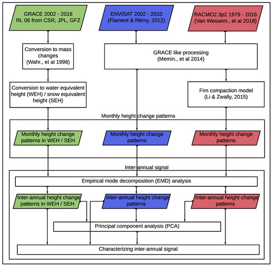
Figure 1.
Flowchart of the study. Parallelogram represents data used and rectangle represents a process. The arrow points towards direction of data flow.
3.1. From Space-Borne Observations
Elevation change has been globally regarded as a robust measure to estimate changes associated with ice sheets. Elevation change data of the AIS exist since the 1990s at a very good spatial and temporal resolution. In our study, we employ a GRACE-like processing on this data to derive monthly maps of elevation changes [25]. Due to the inclination of the orbit, Envisat observations cover the AIS down to 81.5 S. We derive monthly maps of elevation changes on a 1× 1 grid providing 2959 time series. We subtract a degree-2 polynomial fit as we focus on understanding the inter-annual signals and their variability. This degree-2 polynomial represents the trend and the acceleration of present-day ice sheet mass changes resulting from a combination of changes in the height of snow and ice.
We use the average of the three GRACE solutions for the gravity potential as it increases the signal-to-noise ratio of the time series [48]. Observations from the GRACE mission are not only subject to present-day ice-mass loss but also GIA [49]. As for the altimetry processing, we eliminate those contributions by removing a degree-2 polynomial fit. The resulting inter-annual variations in the gravity potential can be converted into mass changes according to the assumption of the thin sheet layer [35]. Mass changes are then converted into water (WEH), ice (IEH), or snow (SEH) equivalent height [26]. Comparing these three variables with height changes from altimetry or modeling helps identifing the nature of the changing mass.
3.2. From Modeling
Preliminary and most defining development on firn compaction models were based on data from ice cores from various ice sheets [50]. Most of these models have been developed based on firn physics and data from ice cores from different ice sheets around the world which has gone through varying climatic conditions [51,52]. They largely employ heat transfer equations alongside the firn densification process. It can portray the transition of snow, with low density, into ice, with high density, over time and depth.
Height changes of an ice sheet at short time scale and not near the coastal area are primarily due to changes in accumulation and temperature [52,53]. Therefore, changes in elevation of an ice sheet can be modeled using accumulation and temperature data or estimates as inputs to a firn compaction model (FCM). We use accumulation and temperature changes from RACMO2.3p2 outputs and the model developed by Stevens et al. (2020) to account for firn compaction [54]. Referring to the implementation by Stevens et al. (2020), we carried out experiments and tests and successfully replicated the results obtained by Li and Zwally (2015) [52,54]. Then, we estimate height changes over the AIS since 1992 as follows.
Inputs to the model include rate of accumulation, density of snow, temperature, rate of melt, etc. We assume a constant snow density across the AIS at 350 kg m. The depth at which firn density is closer to that of the ice varies across the AIS. This depth, which is referred to as critical depth, depends on the climate conditions including rate of accumulation and average temperature. Even though critical depth varies across the AIS, we use a contant firn column of depth 220 m inspired from Verjans et al. (2020) [55]. The rate of densification depends on accumulation rate and temperature changes; consequently, it varies across the AIS, along with the climatic conditions. We also assumed the rate of melt to be nil as it is dominant only close to the coasts, and reliable estimate of it is unavailable. A GRACE-like processing, following that of Mémin et al. [25], is applied to temperature and accumulation fields before running the FCM. A fresh firn column is modeled at each location in which the density at the top will be that of the snow and at the bottom will be that of the ice. The model is pre-initialized for a period (∼100 years) long enough to generate the firn column based upon the currently available climate variables.
In summary, we have derived estimates of height change from Envisat mission (October 2002–October 2010), from GRACE solutions (October 2002–June 2016), and from RACMO outputs combined to a FCM (October 1992–December 2016). Next, we compare the estimated height changes before extracting the inter-annual changes in Section 4.
3.3. Inter-Comparison between Height Change Estimates
We obtained height changes from three different and independent data sets. Comparing each of these estimates with one another is of paramount importance to improve our understanding of mass changes over the AIS. In order to compare the height changes estimated from the three data sets we use, we compute the coefficient of linear regression between time series derived from Envisat and GRACE, Envisat and RACMO, GRACE and RACMO over the common time interval, 2002–2010. This coefficient reflects how well time and amplitude variations of a time series are similar to that estimated from another observation. The coefficient of linear regression, C between two data sets and is given by:
where and represent the coefficient of regression for with respect to , and vice-versa, respectively. i and j stand for the latitude and longitude of the region, respectively. Uncertainty associated, U is expressed as:
where and represent the uncertainty obtained while calculating and , respectively. These coefficients of linear regression and their corresponding uncertainties are mapped in Figure 2a–f.
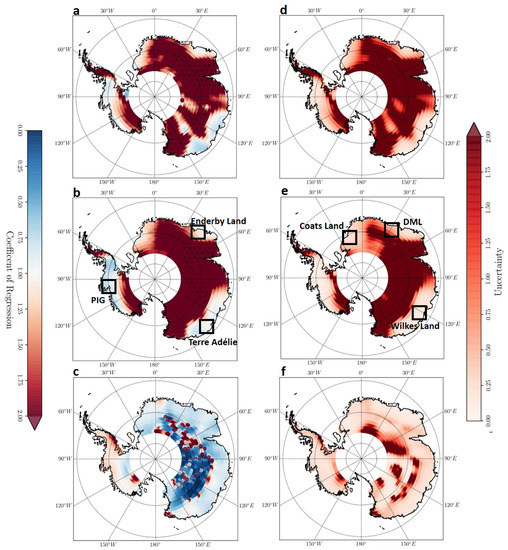
Figure 2.
Coefficient of regression (left) and uncertainty (right) maps between height changes estimated from (a,d) Envisat and GRACE in SEH, (b,e) Envisat and RACMO, and (c,f) GRACE in SEH and RACMO, during the period 2002–2010. In the coefficient of regression maps, color indicates the magnitude, and the dark circle refer to regions where the coefficient is negative. Larger uncertainty values are indicated using dark red.
In an ideal case, the coefficient of regression is close to 1 and the corresponding uncertainty close to 0. A positive coefficient indicates that both estimates of height change increase or decrease together, whereas having a negative coefficient implies the other way around. Along with that, the magnitude of the coefficient characterizes the relation between the amplitude of the signal. A coefficient closer to 1 indicates that height estimates from the two techniques are identical in phase and amplitude. Height changes estimated from GRACE in SEH and those derived from RACMO are close to this ideal scenario (Figure 2c,f). We can also locate regions where it is close to ideal in every map. This include regions in West Antarctica, regions close to Coats Land (CL), Dronning Maud Land (DML), and Wilkes Land (WL) in East Antarctica (Table 1). Whatever the height-change estimates combination, the coefficients are the optimal closer to coastal regions than in-lands, more specifically in East Antarctica where larger uncertainties are present (GRACE—Envisat and Envisat—RACMO).

Table 1.
Regression coefficients between height changes computed using our three data sets at four different locations with respective coordinates in square brackets. Values in the bracket denotes uncertainty.
Height changes for four distant locations (Pine Island Glacier (PIG), CL, DML, WL), where we have near optimal regression coefficients and minimal uncertainties, are shown in Figure 3a–d.
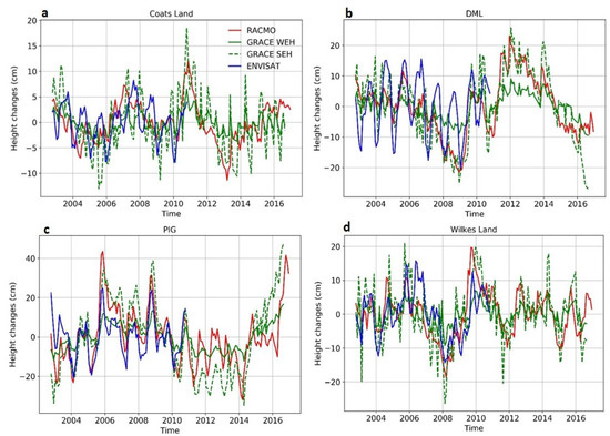
Figure 3.
Height changes are shown for CL (a), DML (b), PIG (c), and WL (d) with that computed from RACMO in red, GRACE solutions in green, separating WEH (solid) from SEH (dash), and Envisat observations in blue. The abscissa is the time. The ordinate shows the amplitude (in cm), which varies in each subplot.
We compare more closely height changes at CL, PIG, DML, and WL. The largest variations in height changes happen in regions around PIG compared to DML, WL and CL. At these four locations, the correlation is between 29 and 63%, 38 and 90%, and 60 and 74% between height changes derived from Envisat and GRACE, Envisat and RACMO, GRACE and RACMO, respectively (Table 2). The lowest correlation is obtained when using height changes from Envisat for CL and DML. Indeed, at these two locations, the seasonal signal in Envisat height changes reaches 10 to 20 cm peak-to-trough and is either lagged (CL) or too important (DML) compared to changes derived from GRACE and RACMO. However, in PIG and WL, the three data sets agree remarkably well between 2002 and 2010 (Figure S1). To investigate the role of the density when computing height changes from GRACE, we convert the changes into WEH and SEH. It indicates that inter-annual SEH changes are in very good agreement with that from RACMO at CL, DML, and WL. However, the smaller periods are slightly too large. At PIG, the seasonal amplitude in SEH changes is slightly smaller than that of RACMO-derived height changes after 2011. An intermediate density between water and snow would lead to a better agreement for the inter-annual signal derived from GRACE and RACMO. Height change estimates from GRACE and RACMO extended to 07/2016 also show a very good correlation at all four locations. In order to better describe and understand the processes competing in Antarctica, we focus next on the time interval common to the three data sets.
Table 2.
Correlation coefficients between height changes computed using our three data sets at four different locations.
4. Extraction of Inter-Annual Signals
Several methods have been adopted to extract the inter-annual signal around Antarctica. For example, Cerrone et al. [56] used a band-pass filter applied on climate parameters above the southern ocean. Autret et al. [57] used an empirical mode decomposition (EMD) to analyze the automatic weather station data at coast. Here, we first apply the EMD to all of our time series covering the AIS. Then, we perform a principal component analysis on time series from selected locations which each represents a 400 km wide area of the data set.
4.1. Empirical Mode Decomposition
The EMD perform self-adaptive decomposition of the signal on the basis of nonlinear functions extracted from the signal itself [58]. EMD decomposes the signal into intrinsic modes which correspond to physical characteristics of the studied signal using a sifting process. This sifting process consists of defining a local phenomenon or feature considering the oscillations of the signal between a maxima and a minima. This procedure is applied iteratively on the original signal to extract constituent modes and their trends.
The EMD applied to height changes in Antarctica during the period 2002–2010 commonly yields 4 to 6 modes. The largest group, representing 65% of our time series, has 5 modes. Time series resulting in 4 and 6 modes represent 33% and 2%, respectively. For a time series with 5 modes, the first mode represents the quasi-monthly disturbances which is largely referred to as noise (Figure S2). Seasonal cycles and signals with periodicity less than or up to one year constitute the second mode. The third mode has periodicity values greater than 1 year. A quasi-4 year cycle dominates the fourth mode. Higher modes constitute components with longer periods [57]. To extract the inter-annual changes, we reconstruct the time series by combining modes which are independent of high frequency changes, seasonal changes and very long-term trends. Therefore, we combine modes 3 and 4 and modes 4 and 5 to reconstruct the inter-annual changes at locations where we have 5 and 6 modes, respectively. We only use the mode 3 where only 4 modes are obtained after the EMD. At each location, we will have the inter-annual signal which is the height change estimates independent of noise, seasonal signal, and very long-term trends. An example of the EMD is given in the Supplementary Materials (Figure S2). The extracted inter-annual signal contains an average of 60% energy of the original signal. The mean contribution is 50%, 56%, and 73% for height changes from Envisat, GRACE, and RACMO, respectively. Maps of distribution for the whole AIS are included in the Supplementary Materials (Figure S3). The resulting inter-annual height changes at CL, PIG, DML, and WL are shown in Figure 4a–d.
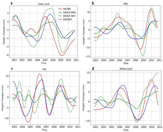
Figure 4.
Inter-annual height changes after mode reconstruction following the EMD analysis at CL (a), DML (b), PIG (c), WL (d). Height change estimates are from RACMO (red), GRACE in WEH (green), SEH (dashed green) and Envisat (blue). The abscissa is the time. The ordinate shows the amplitude of the signal (in cm), which varies in each subplot.
At every selected region, the inter-annual height changes from the three techniques exhibit comparable properties which include period and amplitude. The mean and maximum coefficient of correlation are 63 and 86%, 72 and 91%, and 65 and 91% between inter-annual height changes derived from Envisat and GRACE, Envisat and RACMO, GRACE and RACMO, respectively (Table 3). The inter-annual signal has higher magnitude variations in PIG, DML, and WL, where it has an amplitude of ∼10 cm. In CL, the amplitude of the inter-annual signal falls to ∼5 cm. This difference is likely due to the location of the investigating regions. Indeed, PIG, WL, DML are coastal regions with no permanent ice shelf, whereas CL is close to the permanent Ronne-Filchner ice shelf, thus being likely less subject to ocean influences. Apart from the amplitude, similarities and differences can be derived in terms of periodic content. Indeed, the inter-annual signal in CL, DML, and WL shows longer periods than that at PIG. Next, to characterize the inter-annual changes over the whole of the AIS, we use the reconstructed height changes from the EMD.
Table 3.
Correlation coefficients between inter-annual height changes derived using EMD analysis.
4.2. Characterizing Inter-Annual Changes
To identify the dominant temporal content of our estimated inter-annual changes, we use the least squares method to fit for the best periodic signal. Given a range of periods, distributed monthly from 2 to 8 years, we estimate a single-period model that fits our extracted inter-annual signal. We then compute the Root Mean Square (RMS) of the difference between the derived height changes and the estimated model and select the model that leads to the lowest RMS. If S represents our derived inter-annual changes, and represents the periodic fit with a periodicity of T, then:
where i and j stand for the latitude and longitude of the region, respectively. To assess the outputs of the fitting process across the AIS, we compute the RMS reduction (in %) of our derived inter-annual changes after removing the best fit. RMS reduction is computed using the following relation:
tends to 100% if the model fits perfectly, and 0% otherwise. It is mapped in Figure 5, while the period and the amplitude of the best fitting model are mapped in Figure 6.
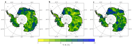
Figure 5.
RMS reduction (in %) of the best single-period fitting model for height changes estimated from Envisat (a), GRACE (b), and RACMO (c).
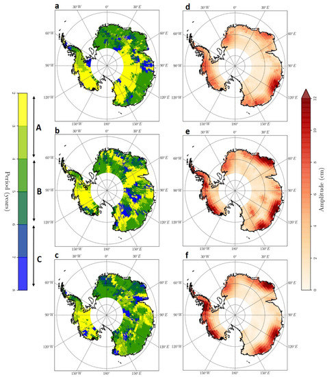
Figure 6.
Maps of the periods (left) and amplitudes (right) of the best fitting model for height changes estimated from Envisat (a,d), GRACE in SEH (b,e), and RACMO (c,f) after EMD. The period range is broken down into three classes: A, B, and C.
Using GRACE, RACMO, or Envisat derived height changes, Figure 5 shows that regions where the RMS reduction is the largest are broadly the same. These regions are that of PIG, CL, WL, Enderby Land (EL, between 30 and 60 E), and Terre Adélie (TA, west of 150 E) (Figure 2). There, the RMS reduction is larger than 50%. It can reach up to 80% in CL and TA. GRACE derived height changes lead to the lowest RMS reduction, while that from RACMO are the largest. Similarly, Figure 6a–c show that the periodic signals that best fit our derived height changes from our three data sets have very similar periods in similar regions, which are those where the RMS reduction is the largest. The amplitude of the best periodic signals are also comparable and reach up to 12 cm (Figure 6d–f).
We find that identical spatial patterns exist for the periodicity maps from our three distinctive data sets. We classify the whole AIS into three regions according to the best fitting periods. These three period classes correspond to areas where periods are: less than 4 years (class A), between 4 and 6 years (class B), and greater than 6 years (class C). The class-wise distribution among each data set is shown in Table 4. The class that covers the largest area is class B, representing 44 to 52% of the total studied area. Regions with latitudes North of 75 S and between 30 W and 165 E (see the period of inter-annual signal in Figure 4a,b,d), barring few exceptional regions, like that of Mac Robertson Land, are dominated by class B. Periods less than 4 years are primarily in West Antarctica (see the period of inter-annual signal in Figure 4c) and in the Antarctic Peninsula. This class A has a total coverage of 40 to 47% of the investigated regions. The final class, and the smallest class, class C, is found at exceptional regions indicating no clear spatial patterns and covers only 8 to 10% area.
Table 4.
Percentage of area covered by each class from each data set.
Amplitude maps show quasi-identical patterns across estimates derived from Envisat, GRACE, and RACMO. The inter-annual signal is the strongest along the coast of the Antarctic Pacific sector and in EL and WL, even though the estimates seem to vary in magnitude depending on the data sets. Comparing amplitude maps of GRACE in SEH and WEH, SEH amplitude map is found comparable in magnitude with that from RACMO and Envisat rather than WEH. It supports the idea that the inter-annual changes are majorly driven by changes in density closer to that of snow. It is also worth noting that the inter-annual signals are greater than an average magnitude along the coasts of the AIS, except in regions between 60 E and 110 E, where it seems to have very less magnitude. The area where the inter-annual signal has significant influence and strength falls within a buffer of ∼600 km or 5 from the AIS coastline. This buffer region shows common periods across different data sets. To explore the inter-annual signal in this region and extract common modes of variability from our three data sets, we perform locally a PCA (Principal Component Analysis) on the height changes.
4.3. Principal Component Analysis
PCA on a multivariate time series is a statistical technique used for deriving the variance-covariance matrix of a set of m—dimensional variables through a few linear combinations of these variables [59]. A large m—dimensional data can be sufficiently expressed by k—principal components, where and, hence, a reduction of the number of degrees of freedom of the problem. It also converts a set of correlated variables into a set of uncorrelated variables through an orthogonal transformation. This technique can be used on general variables or standardized variables and hence either the covariance matrix or correlation matrix is used. The goal of the method is to represent a large m—dimensional process with much smaller k—principal components that would explain a large part of the variance of the data.
We selected longitudinally equally spaced regions (15 apart) along the coast of the AIS and within the buffer region discussed in the previous section (Figure 7a). We perform PCA locally on our three independent time series normalized to their standard deviation and obtained three principal components (PCs): PC1, PC2, and PC3. The first principal component, PC1 has a mean variance of 76% and a standard deviation of 11%. Means of the variance of the second and third principal components (PC2 and PC3) are, respectively, 17% and 6%. We study the first principal component (PC1) as it accounts for the largest part of the variability. Explained variance of PC1 for the whole of the AIS is also shown in Figure 7a. We can clearly see that regions having high variance for PC1 are the same as regions where we have near ideal scenario as explained in Section 3.3. PC1 also accounts for almost equal contributions in the range 0.5 to 0.7 from each of the three data sets except at few locations which include longitudes 60, 75, 165, and 210 E (Table S2 in Supplementary Materials). PC1 obtained locally is plotted in Figure 7b,c. The shaded region located between 165 and 210 E and 285 and 330 E correspond to regions where observations are not considered due to the presence of ice shelves.
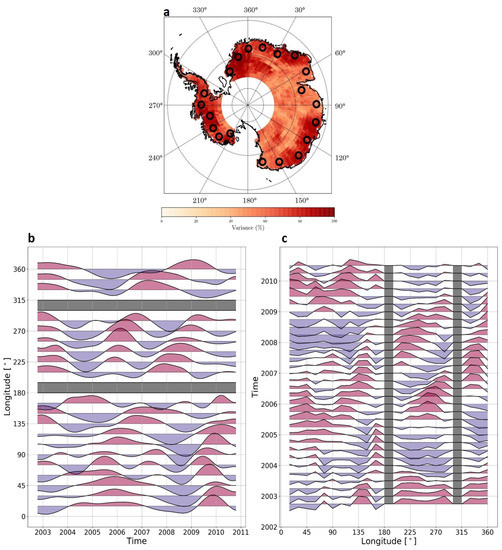
Figure 7.
Explained variance map of the PC1 with locations (black circles) of sites selected to perform the PCA (a). Darker color indicates larger explained variance. Resulting PC1 height changes ordered by longitude (b) and ordered by time (c). The grey colored region represents ice shelves. Positive and negative anomalies are in red and blue, respectively.
A detailed time series analysis of the PC1 shows two positive and two negative anomalies in most of the regions during our period of study. It is consistent with the conclusions obtained in the previous section from Figure 6. Similar patterns are also visible in the spatial analysis. We can also notice a shift, gradually eastward, in the time of occurrence of the positive anomalies in PC1 while circling Antarctica from 15 to 285 E. This feature is clearly seen during the spatial analysis as positive anomalies traverse from 0 to 285 E during the period April 2004–June 2009. Assuming anomalies propagate eastward around the AIS, with a positive anomaly in July 2004 at 15 E and another one in April 2009 at 285 E, the mean propagation rate would suggest that an anomaly takes about 6 years to circle the ice sheet. However, one can notice that the propagation is not constant across the ice sheet. For example, from Figure 7b,c, we can notice that the positive anomaly propagation gets delayed during 2003–2005 close to the Ross ice shelf, whereas there is no such delay during the period 2006–2010. To investigate this further, we estimated the occurrence time of the positive anomalies that are longitudinally successive at each locations based on Figure 7b. The results are summarized in Figure 8.
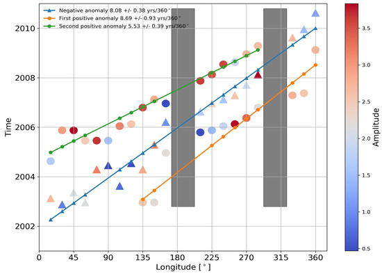
Figure 8.
Time occurrence of anomalies in PC1 that are longitudinally successive around the AIS. Circles and triangles represent positive and negative anomalies, respectively. The color depicts the absolute amplitude of the anomaly at each location from PC1. Linear trends are estimated considering negative anomalies (blue), positive anomalies between 135 and 360 E (orange), and positive anomalies between 15 and 285 E (green), ignoring locations with variance <70%.
The positive anomaly at 15 E longitude from Figure 7b has its first peak in July 2004. This anomaly shows a smooth trend of propagation up to 285 E, in almost 5 years, with 30 and 45 E being two exceptions. Between 15 and 30 E, the positive anomaly appears to be lagged by about one year and seems to circle the rest of the AIS at a quasi-constant rate after 45 E. We have estimated the period to traverse the whole AIS by avoiding the regions where we have explained variance lower than 70% for PC1 (Table S1 in Supplementary Materials). Longitudes 75, 90, 165, and 210 E fall under this category. Therefore, the mean time for encircling the entire AIS is about 5.5 years (green line in Figure 8). We observe maximum amplitude for this anomaly at 45 E. The anomaly is the weakest at 165 E, which is the endpoint of a decreasing trend since 135 E. This also coincides with increasing distance from 65 S, which reaches its maximum at 165 E. The same feature is observed at 255 E, where we have lesser amplitude compared to other sampling locations in the AP sector (210 to 285 E).
We repeat the same analysis with the negative anomalies, as indeed we observe a negative anomaly originating in later half of 2002 at 15 E and propagating eastward till late 2010 at 360 E in Figure 7. Similarly another trend is observed between 135 and 360 E of positive anomalies during December 2002 to January 2009. Both these trends take approximately 7.5 to 9.5 years to traverse across the AIS. As we observe, this phenomenon of propagation of anomalies is a continuous one, and we have not identified any particular starting point and ending point. These anomalies seem to be enhanced or diminished regionally.
5. Discussion
We discuss in this section the possible influence of major climate modes of variability.
5.1. Influence of El Niño Southern Oscillation
ENSO is a climate variability occurring on the timescales of 2–7 years and affecting both the atmosphere and the ocean globally. It supposedly brings along anomalies in SST, sea ice extent, ice shelf thinning rates, and surface melt events in and around AIS [9,10,11]. As it also creates simultaneous high and low pressure systems, leading to larger cloud formation and precipitation, it should affect the AIS.
Sasgen et al. (2010) have discussed the influence of ENSO in mass change patterns using SOI, GRACE solutions, and weather model data [13]. They have found that the inter-annual mass variability along the Antarctic Peninsula and the Amundsen Sea sector, obtained from GRACE, contains ENSO signatures. These mass estimates are exclusive of offset, linear trend, and annual harmonic and are found to be mainly a consequence of accumulation variations governed by changes in precipitation rates. ENSO influence over Antarctic ice shelves is also well discussed using weather and altimetry data by Paolo et al. (2018) [60]. They have been able to link ice-shelf height variability in the AP sector with changes in the regional atmospheric circulation driven by the ENSO with indices including ONI. Mémin et al. (2015) have detected anomalies with a period of about 4–6 years in a combined analysis of surface-mass and elevation changes between August 2002 and October 2010 [14]. Our results suggest at least 44% of the total studied area have periods between 4 and 6 years (class B in Table 4). By using climate model driven height change estimates for our study, we confirm that the inter-annual geodetic anomalies observed in Antarctica are due to changes in atmospheric conditions. Interestingly, Zhan et al. (2021) [61] associated climate related events to dominate mass change trends in AIS by carrying out a complex principal component analysis. The frequency of their primary component matches with our major period class.
Correlation coefficient maps between the ENSO index and inter-annual height changes from Envisat, GRACE, and RACMO reveal the influence of ENSO on height change patterns (Figure 9). Correlation coefficient ranges between −0.7 and 0.7. Positive correlations are commonly found in the East Antarctica beyond 0 up until 130 E. This is the same area where we find inter-annual signals having periods in the range of 4 to 6 years and more than average amplitudes. Maximum positive correlation is obtained in regions around DML and WL, especially when height changes are derived from RACMO and GRACE. Most of the regions in the West Antarctica exhibit negative correlation coefficients, which is consistent with what we observe in the periodicity maps. Zhang et al. (2021) [32] also attributed the inter-annual changes in ice mass over the AIS to precipitation related events associated with ENSO analyzing GRACE data and other mass balance estimates. Even though they limited studies based on regional estimates, they, too, discussed about varying characteristics between East Antarctica and West Antarctica. This is further explained in the upcoming section.
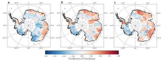
Figure 9.
Correlation maps between ONI and inter-annual height changes estimated from (a) ENVISAT, (b) GRACE, and (c) RACMO. Positive and negative correlation coefficients are in red and blue, respectively.
5.2. Influence of Southern Annular Mode
Apart from the influence of the ENSO, regions in the Pacific sector are subject to other climate drivers, such as the Southern Annular Mode (SAM) and the Amundsen Sea Low (ASL) [62,63]. SAM is the dominant mode of atmospheric variability in the Southern Hemisphere (SH) imposing a major shift in the broad-scale climate of the hemisphere influencing precipitation and temperature on month-to-month and inter-annual timescales [64]. It is quantified based on the zonal pressure difference between the latitudes of 40 S and 65 S. Positive values of the SAM index correspond with stronger-than-average westerlies over the mid-high latitudes (50 S–70 S) and weaker westerlies in the mid-latitudes (30 S–50 S). The influence of ENSO on the AIS is either enhanced or diminished depending upon the phase of SAM [65]. ASL is a climatological low pressure system that exerts considerable influence on the climate of West Antarctica. It influences the wind anomalies, snowfall, temperature patterns, and sea ice extent. Given the broader frequency content of SAM and ASL, these drivers are the likely cause for deviation of period values from class B (4 to 6 years) in West Antarctica and the Antarctic Peninsula. These regions have periods less than 4 years (class A), which may be due to the influence of the SAM or the ASL in phase or out of phase with the ENSO. Depending upon the phase and the time of occurrence, ASL and SAM either strengthen or weaken the ENSO signature. The influence of ASL and SAM is strongly felt along the Amundsen Sea sector, as well as in the Antarctic Pacific sector, which overlaps with above mentioned regions [60].
5.3. Influence of Antarctic Circumpolar Wave
The ACW is a phenomenon where large scale co-varying oceanic and atmospheric anomalies propagate eastward across the Southern Ocean (SO) on subdecadal time scales [15,16,17]. This phenomenon influences weather variables, like SST, sea ice extent, sea level pressure (SLP), and wind velocities, which is similar to what ENSO does.
ACW is commonly found as a wavenumber-2, wavenumber-3, and the Pacific-South American (PSA) pattern in studies associated with a combination of oceanic and atmospheric models [66,67]. A zonal or a hemispheric wavenumber refers to the dimensionless number of wavelengths fitting within a full circle around the globe at a given latitude. Few studies have tried to interlink both ENSO and ACW together [16]. Prior studies investigating the characteristics, origin, effects and propagation of the wave in different time periods summarized the wave as a combination of wave-2 and wave-3 patterns. A wave-2 pattern is more associated with ENSO’s tropical standing mode while a wave-3 pattern comes into play on weakening of the ENSO [68,69,70,71,72]. A wave-2 pattern usually takes around 8 to 10 years to circumnavigate and has a periodicity of 4 to 5 years, which is similar to that of the ENSO phenomenon [15,16].
White and Peterson have found that, in between two ENSO occurrences, the anomalies in temperature and pressure are propagated eastwards by the ACW into the Atlantic and Indian ocean portions of the SO [15]. Long-term studies have also shown inter-decadal changes in the behavior of this wave [56]. These changes are due to tropical and subtropical ocean warming and ozone depletion and variability of El Nino [73,74]. They also categorize change in the wave behavior which includes equatorward expansion to a warmer subtropical south Indian Ocean instead of a warmer subtropical South Pacific Ocean which, with passage of time, becomes cold. Earlier studies have indicated possibilities of weakening and decelerating of the anomaly propagation in the Indian Ocean sector of Antarctica ( to E) due to topographic meandering where the region gets warmer during winter [75].
Ice core records from DML have exposed a 4- to 5-year quasi-periodic signature in sea salt aerosol deposition over 2000 years depicting how ENSO and ACW influence climate in the AIS [71]. This was complemented by a study where an 8-year rotating wave with a 4-year apparent periodicity was observed while analyzing the temperature variations at 10 automatic weather stations around the continent [57]. Anomalies were found in surface mass and elevation change estimated from space-borne geodetic techniques which had a periodicity of 4 to 6 years that circle AIS in 9 to 10 years and thereafter attributed to ACW or ENSO contributions over the AIS [14].
During the characterization phase of the inter-annual signals, we observe above average amplitude values within a buffer of ∼600 km or 5 from the AIS coastline in Figure 6d–f. This buffer region is sampled at equal gaps (15 apart longitudinally) for a combined analysis using three data sets (Figure 7a). The PC1 obtained after a PCA on these normalized data sets explains 76% of the variance and mostly equals contribution from each constituent data set barring a few exceptional regions. A wavenumber-2 pattern is observed at most of the sampling locations (Figure 7b). Our results show anomalies with a dominant periodicity across the AIS in the range of 4 to 6 years. These anomalies show an eastward propagating pattern from 15 to 360 E. The propagating rate indicates that the anomaly encircles the AIS in about 8 years with irregular velocities. Variation in propagation rate can be attributed to local features, including location, topography, and wind velocities. Figure 7c, too, points the presence of a rotating wave which propagates eastwards. These elements favor the effect of the ACW.
6. Conclusions
In this study, we investigated inter-annual variability in the AIS combining multiple geodetic observations (altimetry and gravimetry) and outputs from the regional climate model, RACMO2.3p2. In the process, we estimated height changes from gravity changes based on Wahr et al. (1998) [35] and from weather variables using firn compaction model of Li and Zwally (2015) [52]. This was then combined with elevation changes from Envisat mission for the common period 2002–2010 (Section 3.3) [19]. We then employ EMD technique to extract inter-annual signals which represents an average 60% of the monthly height changes (Figure S3) [57]. During this process, we isolate inter-annual height change patterns by removing noise and components with very high (greater than 0.5 year) and very low (less than 0.125 year) frequencies. We use the least squares method to find the best fitting period and amplitude for this inter-annual signals. Class B (4–6 years) covers the largest portion of the study area, closely followed by class A (<4 years) (Table 4) [14,61].
Period and amplitude maps (Figure 6) indicate the likely influence of inter-annual climatic processes on the ice sheets. Inter-annual signal in the East Antarctica has periods similar to that of ENSO and shows positive correlation up to 0.7 (Figure 9), whereas the trends in West Antarctica and Antarctic Peninsula (Figure 6 and Figure 9) can be explained by the influence of phenomenon, like SAM and ASL, in the AP sector [60]. A PCA of inter-annual signals along the coast at equal intervals also revealed a possible influence of the ACW on the AIS (Figure 7) [14]. ACW seems to carry the climatic anomaly across the AIS, influencing regions along the coast with varying rates of propagation which is dependent on local features (Figure 8). A particular anomaly seems to take 6–8 years to encircle AIS as we observe it in different sectors during our period of study, and its magnitude of influence, too, varies locally.
Further long-term research into the presence and evolution of climate drivers and their possible influence on the AIS is very crucial in factoring these components into global climate models to get better estimates of global mean sea level changes. Quantifying the influence of multiple competing climate drivers is still open for research.
Supplementary Materials
The following are available online at https://www.mdpi.com/article/10.3390/rs13112199/s1, Figure S1: Coefficient of correlation between height changes estimated from (a) Envisat and GRACE, (b) Envisat and RACMO, and (c) GRACE and RACMO, during the period 2002–2010. Figure S2: Overview of the empirical mode decomposition (EMD). Figure S3: Energy ratio of the inter-annual signal extracted from (a) Envisat, (b) GRACE, and (c) RACMO. Table S1: Explained variance in percentage after Principal Component Analysis (PCA). Table S2: Coefficient of each data set in PC1.
Author Contributions
All co-authors have contributed to the data processing and analysis, writing, review, and editing of the paper. All authors have read and agreed to the published version of the manuscript.
Funding
This work has been partly funded by the Center National d’Etudes Spatiales (CNES) through the TOSCA program.
Institutional Review Board Statement
Not applicable.
Informed Consent Statement
Not applicable.
Data Availability Statement
The data presented in this study are available on request from the corresponding author.
Acknowledgments
The authors would like to thank Christopher Max Stevens (University of Washington) for his advice. We are also grateful to the three reviewers for their constructive comments and suggestions, which helped improve the manuscript.
Conflicts of Interest
The authors declare no conflict of interest.
Abbreviations
The following abbreviations are used in this manuscript:
| AIS | Antarctic Ice Sheet |
| GRACE | Gravity Recovery And Climate Experiment |
| SEH | Snow Equivalent Height |
| FCM | Firn Compaction Model |
| CL | Coats Land |
| DML | Dronning Maud Land |
| WL | Wilkes Land |
| PIG | Pine Island Glacier |
| EMD | Empirical Mode Decomposition |
| RMS | Root Mean Square |
| PCA | Principal Component Analysis |
| ENSO | El Niño Southern Oscillation |
| SOI | Southern Oscillation Index |
| ONI | Oceanic Niño Index |
| SAM | Southern Annular Mode |
| ASL | Amundsen Sea Low |
| ACW | Antarctic Circumpolar Wave |
References
- Fretwell, P.; Pritchard, H.D.; Vaughan, D.G.; Bamber, J.L.; Barrand, N.E.; Bell, R.; Bianchi, C.; Bingham, R.G.; Blankenship, D.D.; Casassa, G.; et al. Bedmap2: Improved ice bed, surface and thickness datasets for Antarctica. Cryosphere 2013, 7, 375–393. [Google Scholar] [CrossRef]
- Steig, E.J.; Schneider, D.P.; Rutherford, S.D.; Mann, M.E.; Comiso, J.C.; Shindell, D.T. Warming of the Antarctic ice-sheet surface since the 1957 International Geophysical Year. Nature 2009, 457, 459–462. [Google Scholar] [CrossRef] [PubMed]
- DeConto, R.M.; Pollard, D. Contribution of Antarctica to past and future sea-level rise. Nature 2016, 531, 591–597. [Google Scholar] [CrossRef] [PubMed]
- Stocker, T.F.; Qin, D.; Plattner, G.K.; Tignor, M.; Allen, S.K.; Boschung, J.; Nauels, A.; Xia, Y.; Bex, V.; Midgley, P.M. Climate Change 2013: The Physical Science Basis. Intergovernmental Panel on Climate Change, Working Group I Contribution to the IPCC Fifth Assessment Report (AR5). 2013. Available online: https://boris.unibe.ch/71452/ (accessed on 6 May 2021). [CrossRef]
- Shepherd, A.; Ivins, E.R.; Geruo, A.; Barletta, V.R.; Bentley, M.J.; Bettadpur, S.; Briggs, K.H.; Bromwich, D.H.; Forsberg, R.; Galin, N.; et al. A reconciled estimate of ice-sheet mass balance. Science 2012, 338, 1183–1189. [Google Scholar] [CrossRef] [PubMed]
- Horwath, M.; Legresy, B.; Remy, F.; Blarel, F.; Lemoine, J.M. Consistent patterns of Antarctic ice sheet interannual variations from ENVISAT radar altimetry and GRACE satellite gravimetry. Geophys. J. Int. 2012, 189, 863–876. [Google Scholar] [CrossRef]
- Massom, R.A.; Stammerjohn, S.E. Antarctic sea ice change and variability—Physical and ecological implications. Polar Sci. 2010, 4, 149–186. [Google Scholar] [CrossRef]
- Schneider, D.P.; Okumura, Y.; Deser, C. Observed Antarctic interannual climate variability and tropical linkages. J. Clim. 2012, 25, 4048–4066. [Google Scholar] [CrossRef]
- Boening, C.; Lebsock, M.; Landerer, F.; Stephens, G. Snowfall-driven mass change on the East Antarctic ice sheet. Geophys. Res. Lett. 2012, 39. [Google Scholar] [CrossRef]
- Kwok, R.; Comiso, J.C.; Lee, T.; Holland, P.R. Linked trends in the South Pacific sea ice edge and Southern Oscillation Index. Geophys. Res. Lett. 2016, 43, 10295–10302. [Google Scholar] [CrossRef]
- Deb, P.; Orr, A.; Bromwich, D.H.; Nicolas, J.P.; Turner, J.; Hosking, J.S. Summer drivers of atmospheric variability affecting ice shelf thinning in the Amundsen Sea Embayment, West Antarctica. Geophys. Res. Lett. 2018, 45, 4124–4133. [Google Scholar] [CrossRef]
- Bodart, J.A.; Bingham, R.J. The Impact of the Extreme 2015–2016 El Niño on the Mass Balance of the Antarctic Ice Sheet. Geophys. Res. Lett. 2019, 46, 13862–13871. [Google Scholar] [CrossRef]
- Sasgen, I.; Dobslaw, H.; Martinec, Z.; Thomas, M. Satellite gravimetry observation of Antarctic snow accumulation related to ENSO. Earth Planet. Sci. Lett. 2010, 299, 352–358. [Google Scholar] [CrossRef]
- Mémin, A.; Flament, T.; Alizier, B.; Watson, C.; Remy, F. Interannual variation of the Antarctic Ice Sheet from a combined analysis of satellite gravimetry and altimetry data. Earth Planet. Sci. Lett. 2015, 422, 150–156. [Google Scholar] [CrossRef]
- White, W.B.; Peterson, R.G. An Antarctic circumpolar wave in surface pressure, wind, temperature and sea-ice extent. Nature 1996, 380, 699–702. [Google Scholar] [CrossRef]
- Peterson, R.G.; White, W.B. Slow oceanic teleconnections linking the Antarctic circumpolar wave with the tropical El Niño-Southern Oscillation. J. Geophys. Res. Ocean. 1998, 103, 24573–24583. [Google Scholar] [CrossRef]
- White, W.B.; Simmonds, I. Sea surface temperature–induced cyclogenesis in the Antarctic circumpolar wave. J. Geophys. Res. Ocean. 2006, 111. [Google Scholar] [CrossRef]
- Kerr, A. Topography, climate and ice masses: A review. Terra Nova 1993, 5, 332–342. [Google Scholar] [CrossRef]
- Rémy, F.; Parouty, S. Antarctic ice sheet and radar altimetry: A review. Remote. Sens. 2009, 1, 1212–1239. [Google Scholar] [CrossRef]
- Shepherd, A.; Ivins, E.; Rignot, E.; Smith, B.; Van Den Broeke, M.; Velicogna, I.; Whitehouse, P.; Briggs, K.; Joughin, I.; Krinner, G.; et al. Mass balance of the Antarctic Ice Sheet from 1992 to 2017. Nature 2018, 558, 219–222. [Google Scholar] [CrossRef]
- Cazenave, A.; Dominh, K.; Guinehut, S.; Berthier, E.; Llovel, W.; Ramillien, G.; Ablain, M.; Larnicol, G. Sea level budget over 2003–2008: A reevaluation from GRACE space gravimetry, satellite altimetry and Argo. Glob. Planet. Chang. 2009, 65, 83–88. [Google Scholar] [CrossRef]
- Tapley, B.D.; Bettadpur, S.; Watkins, M.; Reigber, C. The gravity recovery and climate experiment: Mission overview and early results. Geophys. Res. Lett. 2004, 31. [Google Scholar] [CrossRef]
- Landerer, F.W.; Flechtner, F.M.; Save, H.; Webb, F.H.; Bandikova, T.; Bertiger, W.I.; Bettadpur, S.V.; Byun, S.H.; Dahle, C.; Dobslaw, H.; et al. Extending the global mass change data record: GRACE Follow-On instrument and science data performance. Geophys. Res. Lett 2020, 47. [Google Scholar] [CrossRef]
- Tapley, B.D.; Bettadpur, S.; Ries, J.C.; Thompson, P.F.; Watkins, M.M. GRACE measurements of mass variability in the Earth system. Science 2004, 305, 503–505. [Google Scholar] [CrossRef] [PubMed]
- Mémin, A.; Flament, T.; Remy, F.; Llubes, M. Snow-and ice-height change in Antarctica from satellite gravimetry and altimetry data. Earth Planet. Sci. Lett. 2014, 404, 344–353. [Google Scholar] [CrossRef]
- Ramillien, G.; Lombard, A.; Cazenave, A.; Ivins, E.R.; Llubes, M.; Remy, F.; Biancale, R. Interannual variations of the mass balance of the Antarctica and Greenland ice sheets from GRACE. Glob. Planet. Chang. 2006, 53, 198–208. [Google Scholar] [CrossRef]
- Tapley, B.D.; Watkins, M.M.; Flechtner, F.; Reigber, C.; Bettadpur, S.; Rodell, M.; Sasgen, I.; Famiglietti, J.S.; Landerer, F.W.; Chambers, D.P.; et al. Contributions of GRACE to understanding climate change. Nat. Clim. Chang. 2019, 9.5, 358–369. [Google Scholar] [CrossRef]
- Nagler, T. Comprehensive Error Characterisation Report (CECR). Antarctic Ice Sheet CCI Project ESA’s Climate Change Initiative. 2017. Available online: http://www.esa-icesheets-antarctica-cci.org/ (accessed on 6 May 2021).
- Thorvaldsen, A. Product User Guide (PUG) for the Antarctic Ice Sheet CCI Project of ESA’s Climate Change Initiative. Version 1.4. 2018. Available online: http://esa-icesheets-antarctica-cci.org/ (accessed on 6 May 2021).
- Van Wessem, J.M.; Berg, W.J.V.D.; Noel, B.P.; Meijgaard, E.V.; Amory, C.; Birnbaum, G.; Jakobs, C.L.; Kruger, K.; Lenaerts, J.; Lhermitte, S.; et al. Modelling the climate and surface mass balance of polar ice sheets using racmo2: Part 2: Antarctica (1979–2016). Cryosphere 2018, 12, 1479–1498. [Google Scholar] [CrossRef]
- Gao, C.; Lu, Y.; Zhang, Z.; Shi, H. A joint inversion estimate of antarctic ice sheet mass balance using multi-geodetic data sets. Remote. Sens. 2019, 11, 653. [Google Scholar] [CrossRef]
- Zhang, B.; Yao, Y.; Liu, L.; Yang, Y. Interannual ice mass variations over the Antarctic ice sheet from 2003 to 2017 were linked to El Niño-Southern Oscillation. Earth Planet. Sci. Lett. 2021, 560, 116796. [Google Scholar] [CrossRef]
- Wingham, D.J.; Shepherd, A.; Muir, A.; Marshall, G.J. Mass balance of the Antarctic ice sheet. Philos. Trans. R. Soc. A 2006, 364, 1627–1635. [Google Scholar] [CrossRef]
- Flament, T.; Rémy, F. Dynamic thinning of Antarctic glaciers from along-track repeat radar altimetry. J. Glaciol. 2012, 58, 830–840. [Google Scholar] [CrossRef]
- Wahr, J.; Molenaar, M.; Bryan, F. Time variability of the Earth’s gravity field: Hydrological and oceanic effects and their possible detection using GRACE. J. Geophys. Res. Solid Earth 1998, 103, 30205–30229. [Google Scholar] [CrossRef]
- Peltier, W.R. Global glacial isostasy and the surface of the ice-age Earth: The ICE-5G (VM2) model and GRACE. Annu. Rev. Earth Planet. Sci. 2004, 32, 111–149. [Google Scholar] [CrossRef]
- Zwally, H.J.; Li, J. Seasonal and interannual variations of firn densification and ice-sheet surface elevation at the Greenland summit. J. Glaciol. 2002, 48, 199–207. [Google Scholar] [CrossRef]
- Legresy, B.; Papa, F.; Remy, F.; Vinay, G.; Van den Bosch, M.; Zanife, O.Z. ENVISAT radar altimeter measurements over continental surfaces and ice caps using the ICE-2 retracking algorithm. Remote. Sens. Environ. 2005, 95, 150–163. [Google Scholar] [CrossRef]
- Lacroix, P.; Dechambre, M.; Legresy, B.; Blarel, F.; Remy, F. On the use of the dual-frequency ENVISAT altimeter to determine snowpack properties of the Antarctic ice sheet. Remote. Sens. Environ. 2008, 112, 1712–1729. [Google Scholar] [CrossRef]
- Rémy, F.; Mémin, A.; Velicogna, I. Applications of satellite altimetry to study the Antarctic ice sheet. In Altimetry Over Oceans and Land Surfaces (15), 1st ed.; CRC Press: Boca Raton, FL, USA, 2017; p. 670. ISBN 978-1-4987-4345-7. [Google Scholar]
- Cullen, M.J.P. The unified forecast/climate model. Meteorol. Mag. 1993, 122, 81–94. [Google Scholar]
- Undén, P.; Rontu, L.; Jarvinen, H.; Lynch, P.; Calvo Sanchez, F.J.; Cats, G.; Cuxart, J.; Eerola, K.; Fortelius, C.; Garcia-Moya, J.A.; et al. HIRLAM-5 Scientific Documentation; Swedish Meteorological and Hydrological Institute: Norrkoping, Sweden, 2002. [Google Scholar]
- ECMWF. IFS Documentation CY33R1—Part IV: Physical Processes. In IFS Documentation CY33R1; ECMWF: Reading, UK, 2008. [Google Scholar] [CrossRef]
- Rignot, E.; Mouginot, J.; Scheuchl, B.; Van Den Broeke, M.; Van Wessem, M.J.; Morlighem, M. Four decades of Antarctic Ice Sheet mass balance from 1979–2017. Proc. Natl. Acad. Sci. USA 2019, 116, 1095–1103. [Google Scholar] [CrossRef]
- Ropelewski, C.F.; Jones, P.D. An extension of the Tahiti–Darwin southern oscillation index. Mon. Weather. Rev. 1987, 115, 2161–2165. [Google Scholar] [CrossRef]
- Parker, D.E. Documentation of a Southern Oscillation index. Meteorol. Mag. 1983, 112, 184–188. [Google Scholar]
- Huang, B.; Thorne, P.W.; Banzon, V.F.; Boyer, T.; Chepurin, G.; Lawrimore, J.H.; Menne, M.J.; Smith, T.M.; Vose, R.S.; Zhang, H.M. Extended reconstructed sea surface temperature, version 5 (ERSSTv5): Upgrades, validations, and intercomparisons. J. Clim. 2017, 30, 8179–8205. [Google Scholar] [CrossRef]
- Sakumura, C.; Bettadpur, S.; Bruinsma, S. Ensemble prediction and intercomparison analysis of GRACE time-variable gravity field models. Geophys. Res. Lett. 2014, 41, 1389–1397. [Google Scholar] [CrossRef]
- Sasgen, I.; Martinec, Z.; Fleming, K. Regional ice-mass changes and glacial-isostatic adjustment in Antarctica from GRACE. Earth Planet. Sci. Lett. 2007, 264, 391–401. [Google Scholar] [CrossRef]
- Herron, M.M.; Langway, C.C. Firn densification: An empirical model. J. Glaciol. 1980, 25, 373–385. [Google Scholar] [CrossRef]
- Ligtenberg, S.R.M.; Helsen, M.M.; Van den Broeke, M.R. An improved semi-empirical model for the densification of Antarctic firn. Cryosphere 2011, 5, 809–819. [Google Scholar] [CrossRef]
- Li, J.; Zwally, H.J. Response times of ice-sheet surface heights to changes in the rate of Antarctic firn compaction caused by accumulation and temperature variations. J. Glaciol. 2015, 61, 1037–1047. [Google Scholar] [CrossRef]
- Rémy, F.; Parrenin, F. Snow accumulation variability and random walk: How to interpret changes of surface elevation in Antarctica. Earth Planet. Sci. Lett. 2004, 227, 273–280. [Google Scholar] [CrossRef]
- Stevens, C.M.; Verjans, V.; Lundin, J.; Kahle, E.C.; Horlings, A.N.; Horlings, B.I.; Waddington, E.D. The Community Firn Model (CFM) v1.0. Geosci. Model Dev. 2020, 13, 4355–4377. [Google Scholar] [CrossRef]
- Verjans, V.; Leeson, A.A.; Nemeth, C.; Stevens, C.M.; Kuipers Munneke, P.; Noel, B.; van Wessem, J.M. Bayesian calibration of firn densification models. Cryosphere 2020, 14, 3017–3032. [Google Scholar] [CrossRef]
- Cerrone, D.; Fusco, G.; Cotroneo, Y.; Simmonds, I.; Budillon, G. The antarctic circumpolar wave: Its presence and interdecadal changes during the last 142 years. J. Clim. 2017, 30, 6371–6389. [Google Scholar] [CrossRef]
- Autret, G.; Rémy, F.; Roques, S. Multiscale analysis of Antarctic surface temperature series by empirical mode decomposition. J. Atmos. Ocean. Technol. 2013, 30, 649–654. [Google Scholar] [CrossRef]
- Huang, N.E.; Shen, Z.; Long, S.R.; Wu, M.C.; Shih, H.H.; Zheng, Q.; Yen, N.C.; Tung, C.C.; Liu, H.H. The empirical mode decomposition and the Hilbert spectrum for nonlinear and non-stationary time series analysis. Proc. R. Soc. Lond. Ser. A 1998, 454, 903–995. [Google Scholar] [CrossRef]
- Wei, W.W. Multivariate Time Series Analysis and Applications; John Wiley and Sons: Hoboken, NJ, USA, 2018; pp. 139–161. [Google Scholar]
- Paolo, F.S.; Padman, L.; Fricker, H.A.; Adusumilli, S.; Howard, S.; Siegfried, M.R. Response of Pacific-sector Antarctic ice shelves to the El Niño/Southern oscillation. Nature Geosci. 2018, 11, 121–126. [Google Scholar] [CrossRef] [PubMed]
- Zhan, J.; Shi, H.; Wang, Y.; Yao, Y. Complex Principal Component Analysis of Antarctic Ice Sheet Mass Balance. Remote Sens. 2021, 13, 480. [Google Scholar] [CrossRef]
- Raphael, M.N.; Marshall, G.J.; Turner, J.; Fogt, R.L.; Schneider, D.; Dixon, D.A.; Hosking, J.S.; Jones, J.; Hobbs, W.R. The Amundsen sea low: Variability, change, and impact on Antarctic climate. Bull. Am. Meteorol. Soc. 2016, 97, 111–121. [Google Scholar] [CrossRef]
- Hosking, J.S.; Orr, A.; Marshall, G.J.; Turner, J.; Phillips, T. The influence of the Amundsen–Bellingshausen Seas low on the climate of West Antarctica and its representation in coupled climate model simulations. J. Clim. 2013, 26, 6633–6648. [Google Scholar] [CrossRef]
- Marshall, G.J. Trends in the Southern Annular Mode from observations and reanalyses. J. Clim. 2003, 16, 4134–4143. [Google Scholar] [CrossRef]
- Fogt, R.L.; Bromwich, D.H.; Hines, K.M. Understanding the SAM influence on the South Pacific ENSO teleconnection. Clim. Dyn. 2011, 36, 1555–1576. [Google Scholar] [CrossRef]
- Christoph, M.; Barnett, T.P.; Roeckner, E. The Antarctic Circumpolar Wave in a coupled ocean-atmosphere GCM. J. Clim. 1998, 11, 1659–1672. [Google Scholar] [CrossRef]
- Mo, K.C.; White, G.H. Teleconnections in the southern hemisphere. Mon. Weather. Rev. 1985, 113, 22–37. [Google Scholar] [CrossRef]
- White, W.B.; Cherry, N.J. Influence of the Antarctic circumpolar wave upon New Zealand temperature and precipitation during autumn–winter. J. Clim. 1999, 12, 960–976. [Google Scholar] [CrossRef]
- White, W.B. Influence of the Antarctic Circumpolar Wave on Australian precipitation from 1958 to 1997. J. Clim. 2000, 13, 2125–2141. [Google Scholar] [CrossRef]
- Connolley, W.M. Long-term variation of the Antarctic Circumpolar Wave. J. Geophys. Res. Ocean. 2002, 107. [Google Scholar] [CrossRef]
- Fischer, H.; Traufetter, F.; Oerter, H.; Weller, R.; Miller, H. Prevalence of the Antarctic Circumpolar Wave over the last two millenia recorded in Dronning Maud Land ice. Geophys. Res. Lett. 2004, 31. [Google Scholar] [CrossRef]
- Cai, W.; Baines, P.G. Forcing of the Antarctic Circumpolar Wave by El Niño-Southern Oscillation teleconnections. J. Geophys. Res. Ocean. 2001, 106, 9019–9038. [Google Scholar] [CrossRef]
- Bian, L.; Lin, X. Interdecadal change in the Antarctic Circumpolar Wave during 1951–2010. Adv. Atmos. Sci. 2012, 29, 464–470. [Google Scholar] [CrossRef]
- White, W.B.; Annis, J. Influence of the Antarctic Circumpolar Wave on El Niño and its multidecadal changes from 1950 to 2001. J. Geophys. Res. Ocean. 2004, 109. [Google Scholar] [CrossRef]
- Nuncio, M.; Luis, A.J.; Yuan, X. Topographic meandering of Antarctic Circumpolar Current and Antarctic Circumpolar Wave in the ice-ocean-atmosphere system. Geophys. Res. Lett. 2011, 38. [Google Scholar] [CrossRef]


Publisher’s Note: MDPI stays neutral with regard to jurisdictional claims in published maps and institutional affiliations. |
© 2021 by the authors. Licensee MDPI, Basel, Switzerland. This article is an open access article distributed under the terms and conditions of the Creative Commons Attribution (CC BY) license (https://creativecommons.org/licenses/by/4.0/).