Abstract
The effective normalized radar cross section (NRCS) of breaking waves, , is empirically derived based on joint synchronized Ka-band radar and video records of the sea surface from a research tower. The is a key parameter that, along with the breaker footprint fraction, Q, defines the contribution of non-polarized backscattering, NP , to the total sea surface NRCS. Combined with the right representation of the regular Bragg and specular backscattering components, the NP component is fundamental to model and interpret sea surface radar measurements. As the first step, the difference between NRCS values for breaking and non-breaking conditions is scaled with the optically-observed Q and compared with the geometric optics model of breaker backscattering. Optically-derived Q might not be optimal to represent the effect of breaking waves on the radar measurements. Alternatively, we rely on the breaking crest length that is firmly detected by the video technique and the empirically estimated breaker decay (inverse wavelength) scale in the direction of breaking wave propagation. A simplified model of breaker NRCS is then proposed using the geometric optics approach. This semi-analytical model parameterizes the along-wave breaker decay from reported breaker roughness spectra, obtained in laboratory experiments with mechanically-generated breakers. These proposed empirical breaker NRCS estimates agree satisfactorily with observations.
1. Introduction
Co-polarized sea surface radar backscattering are now well documented and understood. Various asymptotic approaches and their combinations, see, e.g., reviews [1,2,3], can help to reproduce observed normalized radar cross-section (NRCS) measurements rather accurately. These approaches are mainly based on the Gaussian assumption for the sea surface statistics, but can account for its non-Gaussian corrections for more advanced analyses [4,5,6,7,8,9]. Alternatively, sea surface non-Gaussian features can be explicitly introduced by separating a wave breaking contribution [10,11]. This helps to explain some of the sea surface NRCS properties that are not consistent with the pure Bragg theory, e.g., anomalous polarization ratio [12], cross-section modulation phase [13,14,15], and upwind-downwind asymmetry [8].
This breaking wave contribution is critical at grazing look geometry and/or HH-polarization when the regular surface backscattering is weak, e.g., for marine radars [16,17]. For small to moderate incidence angles, the net contribution of breaking waves is generally not dominant, but still distinguishable. When considering this contribution as a signal, not just a correction, one may extract this breaker-related backscattering component and thus possibly evaluate the characteristics of breaking waves on global scales from satellite radar data. For high resolution measurements, the wave breaking parameters are sensitive to wave-current, wave-bottom, and wave-wind interactions that can often be well traced. The contribution of wave breaking to the sea surface NRCS can be extracted from a combination of co-polarized NRCS components (polarization difference and ratio) given that wave breaking produces a non-polarized backscatter signal [18,19,20,21,22].
Still, the backscattering mechanism from a breaking wave surface is much less understood than that from a regular, non-breaking surface. It is generally accepted that visible wave breakers and steep crests both provide the so-called radar sea spikes [12,23,24,25,26,27,28,29]. Along with that, laboratory measurements suggest that Ka-band NRCS attenuates in turbulent wakes following active breaking crests, due to small-scale roughness dissipation in turbulent patches [30]. The concept of radar sea spikes is generally applicable for moderate to high incidence angles. For very small incidence angles, the rough breaking patches are expected to have a lower NRCS than the smooth regular surface (so-called contrast inversion that is not yet detected experimentally). Numerous laboratory experiments have been done to investigate wave breaking radar signatures [31,32,33,34,35,36,37,38,39,40,41], but their results are not easily applicable to the real sea surface due to the scaling of wind and wave fields in a tank.
This paper focuses on the evaluation of breaking surface NRCS in the Ka-band, the frequency band selected for the future Doppler scatterometer mission [42]. For this, we rely on field experiment data from a static oceanographic platform that was previously used for Ka-band backscattering investigations [43,44,45,46]. Many of these radar records are accompanied by synchronous video recordings of the sea surface radar footprint. Joint analyses of radar and video signatures of wave breakers then provide experimental means for direct estimation of the NRCS associated with individual breakers in the Ka-band.
2. Data and Methods
2.1. Experiment and Instruments
The experiments were conducted in 2009–2013 from the Black sea research platform ( N, E) moored 600-m offshore in 30-m deep water. The deepwater wave approximation is well applicable to waves at the platform site for a typical wave peak wavelength of approximately 40 m.
A Ka-band dual co-polarized continuous-wave real aperture radar was used in the experiments. Its -3dB two-way antenna beamwidth is about 10/15 in horizontal/vertical plane for VV/HH transmit-receive polarization. More details on the radar calibration and platform experiment techniques can be found in [43,44,45,46]. The radar was mounted on either the top (6.5-m height, incidence angle, ) or the bottom deck of the platform (13-m height, ). The incidence angle, , was varied from to . The radar-to-wind azimuth, , was changed from upwind to downwind.
A full-HD (1440 × 1080 pixels, 25 fps) video camera was used for imaging the radar footprint. For the vast majority of the records, the camera was installed on top of the radar and co-aligned with its beam. Several records were made in a double-look mode with the radar installed on the bottom deck and the camera installed on the top deck, with both looking at the same point on the surface. The camera was synchronized with the radar using the camera audio channel that was recorded by the radar acquisition system. The cross-correlation of radar and video camera audio signals was further used to synchronize radar and video records.
2.2. Radar Data Processing
The description of Doppler processing of our radar data is described in e.g., ref. [44] and briefed below for reader convenience. Raw records contain the digitized demodulated in-phase, I, and quadrature, Q, components of VV- and HH-polarization radar signal sampled at 40 kHz rate. Instantaneous Doppler spectra, , were computed over a 0.2-s running window, where the width is chosen as a tradeoff between noise and temporal resolution. Subseuently, the instantaneous NRCS, , is the running signal variance, , which is proportional to the received power multiplied by a calibration factor.
The Doppler velocity of a target, , is determined directly from the instantaneous Doppler frequency, , obtained from instantaneous spectra, as, , where cm is the radar wavelength.
2.3. Video Data Processing
To save computational time, the video processing was performed in two steps: (i) detecting individual breaking events from all video data; and, (ii) analyzing breaker characteristics from selected video data sequences for particular breaking events.
First, the synchronized video records were projected on the horizontal plane based on known camera look geometry and subdivided into 5-min. records. The record-averaged image intensity was subtracted from each frame intensity to correct for inhomogeneous background sea surface brightness (due to changes in Fresnel reflection coefficient and reflected sky brightness).
For each 5-min. record, the threshold value for breaker detection in the background-corrected images was selected manually based on visual inspection of the detection result. Using this threshold, the video images were binarized (whitecap and non-whitecap, 1 and 0, respectively). This empirically chosen brightness threshold allows to match the whitecap coverage inferred from the video data with the whitecap wind dependence observed in [47]. The relative area of whitecap pixels within the radar sea surface footprint gives an instantaneous whitecap radar footprint fraction, Q,
where is the binarized image brightness, is the measured two-way radar antenna pattern projected onto the mean sea horizontal plane, and is the distance from the radar to -point on the surface.
The wave breaking process is conventionally divided into an active, phase A, and a passive, phase B, stages [48]. The phase A involves “plunging aerated plumes” or “dynamic foam”, while the phase B is related to “residual foam” that has a patchy, strip-like structure. Our whitecap detection video processing is intended to select the active breaking phase A. The resulting from the first step (Figure 1) is based on all collected video data and lies between the active (A) and total (active plus passive, A + B) empirical whitecap coverage wind dependencies of [47]. Figure 1 suggests that our manual threshold selection, despite possible overestimation at light winds, confidently detects the active phase and partly includes the passive foam.
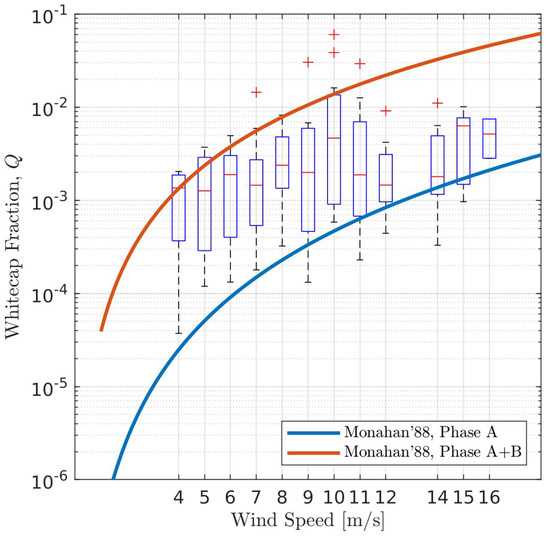
Figure 1.
Whisker plot of whitecap fraction, Q, versus wind speed from the processing step (i) of all video data. The range of each box shows the 25th and 75th percentiles of each wind sample. Red strokes are sample medians, dashed lines (whiskers) are observation spread. Red crosses are outliers distant the interquartile range from box bounds. The solid lines are empirical laws [47].
In our experience, still contains spurious whitecap detections due to glints, remaining foam, and/or floating debris. However, apparent whitecaps dominate and they can be further separated from spurious whitecaps by an additional selection of time steps with . To ease the clustering of temporal video frame sequences based on their correspondence to a particular whitecap, each point of with was extended in time within -s intervals using the morphological dilation procedure [49]. This dilation helps to regularize the clustering procedure and select record intervals that correspond to individual whitecaps.
The second processing step is performed for each breaking event. During the lifetime of a particular whitecap, a set of binarized video frames associated with this event was again analyzed using the Matlab Image Processing Toolbox to measure the geometric characteristics of the detected breakers (binary regions). The temporal evolution of whitecap geometric properties—area, S, major axis length, L, centroid coordinates, X—was retrieved. If a whitecap event contains more than one breaking regions (Figure 2), the radar footprint fraction covered by the i-th region, , was evaluated using Equation (1). Next, the centroid coordinates of all regions were footprint averaged,
where x is a geometric parameter and n is the number of detected regions in the frame taken at time, t.
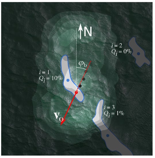
Figure 2.
Sketch of the whitecap detection algorithm showing a sample sea surface video image with radar footprint (higher brightness) overlain. Three whitecap regions detected within the video image cover 10% (), 1% (), and 0% () of the footprint, respectively. Whitecap region centroids are marked by blue circles. The footprint-averaged centroid of the three regions is shown by the red circle. Note, the second region locates outside the footprint and does not contribute (). In this example, the contribution by the first region dominates and it is 10 times larger than . The black circles indicate previous centroid positions that form the footprint-averaged whitecap trajectory. The instantaneous optical velocity, , is tangent to the trajectory.
For each breaking region, the centroid velocity, C, was calculated as the time derivative of this region centroid coordinates. Subsequently, the whitecap event velocity was estimated by footprint averaging of all the regions detected in the frame. The direction of this vector is the instantaneous breaker propagation direction, .
Event-mean characteristics were estimated based on the whitecap footprint fraction, Q, weighted averaging
where x is any geometric parameter (whitecap area, S, length, L, speed, C, or footprint fraction, Q) corresponding to a particular event, the overline is the time average over the event span. The total number of events is about 1000 for all look geometry configurations and environmental conditions.
3. Results
3.1. NRCS Versus Whitecap Fraction
In order to demonstrate whitecap contribution to sea surface radar backscattering, the observed NRCS, , is shown as a function of whitecap fraction, Q. Figure 3 shows all of the instantaneous NRCS values without separation on events, i.e., one event may correspond to several points on this plot. Altough the observed values of Q are quite low, generally below 10% of the effective footprint area, there is a clear positive correlation between and Q (Figure 3a) that reflects an increase in NRCS due to breaker reflections. The maximum instantaneous fraction ∼0.5 was observed with radar and camera orientation at .
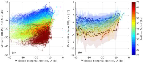
Figure 3.
(a) Observed normalized radar cross-section (NRCS) and (b) bin-averaged polarization ratio, , versus whitecap footprint fraction, Q, for various (color-coded) incidence angles, .
Figure 3b presents the polarization ratio, , computed using the data that are shown in Figure 3a. At low , the PR gradually decreases with increasing . This incidence angle behavior is in line with the resonant Bragg scattering mechanism from the regular, non-breaking sea surface. At larger , the relative contribution of breaker backscattering increases, and the PR increases towards the limiting case that corresponds to non-polarized breaker backscattering (, or 0 dB) for all .
For breaking events with , the measured NRCS is on average 5–7 dB higher than the corresponding 5-min. mean NRCS that represents the background backscattering conditions surrounding each breaking event (Figure 4b,c). The difference between the two reflects the contribution from breaking events. The incidence angle dependence of the NRCS measured during breaking events (Figure 4a) is similar to that derived from the empirical background Ka-band NRCS model [43] shown here for the most frequent observation conditions: upwave, 10 ms wind speed. NRCS record samples that include breakers have systematically higher backscattering values than the model that describes the mean sea surface, both breaking and non-breaking (Figure 4a, symbols versus lines). The maximum difference reaches 10–15 dB for the largest observed Q.
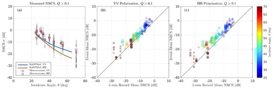
Figure 4.
(a) Observed NRCS measured at footprint fractions, , versus incidence angle, . Lines show the empirical KaDPMod [43] background NRCS. Gray shades show the HH-polarization NRCS points spread, with artificial noise in for better visualization. Model data are shown for the most frequent observation conditions: upwave, 10 ms wind speed. Scatterplots of event mean and 5-min. mean NRCS for (b) VV and (c) HH polarization for various (color-coded) incidence angles, . Symbol size is proportional to wind speed. Symbol transparency is proportional to whitecap footprint fraction, Q.
3.2. Background Estimation
From the available field radar measurements, it is virtually impossible to directly estimate the pure breaking wave cross-section because of relatively low whitecap footprint coverage, Q. This means that the radar backscattering from the regular, non-breaking sea surface largely dominates in our measurements.
The idea of the following analysis is to estimate the background sea surface NRCS, , which corresponds to non-breaker conditions. It is expected that a simple mean of NRCS subsets without breakers will not work as a proxy for the background backscattering because of the presence of long wave modulations (LW) of the illuminated area. Next, we use the radar Doppler velocity as a proxy for LW orbital wave velocity that can further be converted into any parameter of modulating LW (e.g., amplitude, slope, phase) [44].
In the Fourier frequency domain, the wave orbital (Doppler) velocity, , reads
where is the wave elevation, is the wave radial frequency, is the incidence angle, and is the radar-to-wave azimuth.
Binning the NRCS by the estimated LW phase, , one can access and visualize the NRCS modulation by long waves. Partitioning these data with either the smallest or largest footprint fractions yields NRCS estimates for the background whitecap-free and whitecap-covered surfaces. We use the lowest and highest 15% of Q-samples, and , to partition between the two cases. As an example of such analysis, Figure 5 shows three upwind-oriented radar records made in similar 10–11 m/s wind speed conditions, but at different incidence angles, and .
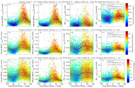
Figure 5.
Long wave profiles of (a,e,i) VV, (b,f,j) HH NRCS, (c,g,k) polarization difference (PD = VV-HH), and (d,h,l) polarization ratio (PR = HH/VV). Symbol color indicates estimated long wave slope for (a–d) , (e–h) , and (i–l) .
A comparison of LW-profiles of the NRCS for mean and whitecap conditions (black and red lines in Figure 5, 1st and 2nd column) indicates a clear peak located ∼30 leeward of the wave crest (forward wave slopes) in the whitecap subset. As expected, the mean NRCS is higher for VV than for HH polarization, but the excess that is associated with wave breaking is of the same magnitude for both polarizations indicating a non-polarized nature of breaker radar backscattering. This is confirmed by LW-profiles of the polarization ratio, , (Figure 5d,h,l) that displays a near-crest peak similar to that in the NRCS. The polarization difference, , normally associated with Bragg-like backscatter only, does not essentially differ between the mean and whitecap subsets, again suggesting the presence of non-polarized (NP) backscattering from breaking areas.
Although there are many clear NP backscattering episodes (), the mean whitecap PR along LW-profile does not reach because the whitecap footprint fraction is normally much less than 1.
The background NRCS, , is estimated for every record from the non-breaking subset (blue lines in Figure 5) using the relation between and following from the Hilbert transform,
where is the time mean NRCS, is the Hilbert transform of the centered Doppler velocity signal, is the Hilbert transform of the centered NRCS “expressed” in logarithmic units to better reproduce the strong non-linearity of the MTF [45], and is the average over the background subset. The M coefficient is a sort of modulation transfer function (MTF) relating variations of the NRCS (in logarithmic units) with the orbital (Doppler) velocity.
3.3. Whitecap NRCS
In order to estimate the pure whitecap NRCS, , it is assumed that whitecap and background scatterers are non-coherent and contribute independently to the total NRCS with the weights defined by the whitecap footprint fraction,
Given known , the pure whitcap NRCS is
Taking into account that whitecap backscattering is almost non-polarized, the analysis focuses mainly on HH data. To minimize noise, the events with low whitecap footprint coverage, , that have only a weak contribution to the are discarded. For each breaking event, the mean is computed as Q-weighted average. Subsequently, all of breaking events data are averaged for a given using Equation (3) (Figure 6).
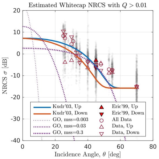
Figure 6.
Estimated whitecap NRCS, , versus incidence angle, . Gray shades show the spread of observed at HH-polarization (some spread is artificially added to observed for better visualization). Filled red triangles show Ericson et al. (Eric’99) [35] laboratory breaker NRCS measurements. Dashed lines show the Geometric Optics (GO) for various mean-square slopes (mss). Solid lines show the Kudryavtsev et al. (Kudr’03) [10] breaker NRCS parameterization.
The resulting estimates of whitecap NRCS are apparently ∼10 dB higher than the measured NRCS even at relatively high (compare Figure 4 and Figure 6). They are also in good agreement with the only, to the best of our knowledge, calibrated X-band breaker NRCS from stationary mechanically-generated breakers measured in a tank that was reported by Ericson et al. [35]. The scatter of estimates is noticeably stronger that the scatter of NRCS measurements (Figure 4 and Figure 6, gray shades). This enhanced scatter is explained by the dependence of on two additional parameters, Q and , which uncertainties lead to apparently stronger variability of estimates. Secondly, the wave breaking is a very sporadic process. In our experience, two optically similar breaking events may produce very different NRCS signatures (see the supplemental video).
Grouping data by the incidence angle reveals interesting, but unexpected, azimuth distributions of whitecap NRCS (Figure 4, compare different triangle symbols). At , the observed upwave/downwave asymmetry is quite weak or noisy, while at small the downwave whitecap NRCS is higher than the azimuth mean and upwave whitecap NRCS. Figure 7b shows more details on data coverage and characteristics of azimuth distribution of the breaker NRCS, which shows the normalized by its mean value for each group. For comparison, we also show NRCS measurements at (by analogy to Figure 4) that are arranged in the same way (Figure 7a).
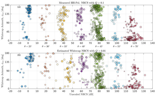
Figure 7.
Azimuth dependence of (a) measured NRCS for and (b) estimated whitecap NRCS, , normalized by the mean NRCS for given . Data cloud points are color-coded, depending in the incidence angle, . Data clouds are shifted along x-axis for better visualization. Azimuth angles and correspond to upwave and downwave directions, respectively. The data cloud slope with respect to the x-axis corresponds to negative (upwave < downwave) and positive (upwave > downwave) asymmetry for acute and obtuse slope angles, respectively.
Unfortunately, the available azimuth statistics is quite poor, with somewhat better coverage only at . In general, the scatter of within -groups is stronger than their azimuth dependence (Figure 7b).
Despite the poor statistics, a negative (upwave<downwave) asymmetry is distinguishable at 20–30. For data points at , a weak, 3–5 dB, increase is present in the upwave direction. Regardless of the strong data point scatter, this upwind increase is distinguishable and in line with the positive (upwave > downwave) 3 dB ratio reported in [35].
At larger 60–70, the asymmetry is not confidently distinguished within the data spread. One of the reasons for this is that Doppler velocity is no longer a good proxy for wave orbital velocity. In our previous study based on these same data [44], a good agreement between long wave characteristics that are retrieved from Doppler velocity and in-situ data from wire wave gauge was present only for . Thus, the background NRCS estimates and resulting may be not accurate at due to weaker Bragg scattering and stronger impact of spikes on the Doppler velocity.
3.4. Comparison with Models
As a first guess for breaking wave backscattering model, the geometric optics (GO) approximation is used,
with the mean square slope (MSS), , as a variable, and is the Ka-band reflection coefficient for power at . However, the GO model fits our estimates only for rather large MSS, , (Figure 6, dashed lines). Additionally, the pure GO model does not account for the upwave/downwave NRCS asymmetry.
Based on the GO approximation, Kudryavtsev et al. [10] (KHCC) proposed a parameterization for breaking wave NRCS, in which the upwind-downwind asymmetry is accounted for by the mean leeward tilt, , of breakers. In this parameterization, the GO model is augmented by a term that is associated with the backscattering from a cylindrical plunging feature atop of breaking crests that accounts for breaking wave contribution at large incidence angles,
where is the mean breaking surface slope, is the beaker MSS, and is the constant depending on breaker thickness to length ratio. Fitting this model to radar observations in various frequency bands (see [10] for details) suggests , , and .
In general, the empirical KHCC parameterization works better than the plain GO model and it compares better with derived from our observations (Figure 6, solid lines). Additionally, note that the KHCC parameterization predicts only positive upwave/downwave asymmetry values independent of .
4. Discussion
The observed inconsistencies motivate us to improve the breaker radar model. The KHCC only describes the forward slope of a breaking wave while the rear slope is not fully considered. From a preliminary analysis of Doppler breaker signatures [50] as well as visual observations of whitecaps, it is known that the breaking wave crest moves at approximately the phase velocity of breaking wave but the breaker roughness is embedded into the water and hence lags behind the crest, gradually dissipates, and then extends to the rear slope of breaking wave. These qualitative considerations provide a clue for a possible explanation of the negative up/downwave breaker NRCS asymmetry at small that may be associated with roughness decay along breaking wave profile and smoother rear slopes.
Moreover, the roughness patch trailing a breaker has less entrained air and, thus, is visually darker than the active whitecap phase normally solely associated with the whole breaking event. As a result, the breaker “seen” by a microwave radar, even in the Ka-band, may differ from the breaker seen by an optical sensor. This is due to substantial variations of the breaker roughness and NRCS within its area. Depending on the incidence angle and azimuth, the non-planar geometry of breaking waves makes either their forward or rear slopes dominating the backscattering. Thus, the NRCS averaged over an optical whitecap feature, even if we could measure it directly at , may differ from the NRCS that is averaged over a radar-detected breaking feature. To avoid discrepancies that are related to the difference between optical and radar breaker footprint fractions, an alternative way of breaking wave characterization is used below. It is based on description of the wave breaking events using length of the breaking crest, a -function, as suggested by Phillips [51].
Consider a breaker that moves with the wave phase speed, C, and it has the breaking crest length per unit surface area, . Subsequently, the surface area fraction swept by this breaker during its life span, , is,
As an alternative to the whitecap footprint fraction, Q, the above equation defines the breaker footprint fraction, q, as seen by a radar. It can be calculated from available direct measurements of C and . Following the hypothesis of self-similarity of breaker and breaking wave parameters [51], the breaker lifetime, , should be proportional to the inverse wave frequency: , and, hence, , where K is the breaking wave wavenumber and is a constant of the order of 1 (e.g., according to field measurements of Korinenko et al. [52], personal communication). Further, this empirical constant is set to, , and the radar breaker footprint fractions is defined as,
where , the fraction of breaker length, L, illuminated by the radar, and , the breaker wavenumber, are estimated from the measurements using Equation (3).
Subsequently, the whitecap NRCS, Equation (8), converts to the breaker NRCS.
Because accounts for the full sea surface breaker coverage, it is expected to be larger than Q, which decreases the estimated breaker NRCS, . To account for the above observed features the following phenomenological breaker backscattering model is proposed.
4.1. Breaker Radar Model
Let us represent the surface elevation of breaking wave as a superposition of carrying wave, , and disturbances, , generated by breaking crest (Figure 8),
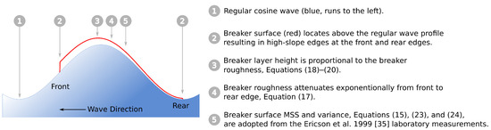
Figure 8.
Sketch of sea elevation in a breaking wave and key points of the breaker radar model.
Because these breaker-induced disturbances are produced by a water mass separating from the breaking crest, their mean level is non-zero. They originate on the forward slope of breaking wave and gradually dissipate, expanding on the rear slope. To provide a realistic and consistent description of breaking wave parameters, an empirical breaking crest isotropic roughness spectrum that was suggested in [35] is adopted:
where is a constant relating the roughness peak wavenumber to the breaking wave wavenumber K, and is a dimensional constant [35].
In the reference frame moving with the breaking wave propagating against the x-axis, the location of the wave crest corresponds to . The source of breaker-induced disturbances is located on the forward slope of the breaking wave and is distributed between to , where is the breaking wave wavelength. On the rear slope, the breaker-induced disturbances decay exponentially and they are assumed to completely disappear after some characteristic time (the breaker life span, ). Subsequently, the spatial distribution of breaker-induced roughness is described as,
where describes spatial variations of breaker-induced roughness during its life span, is the Heaviside step function, r is the dimensionless attenuation scale, and , where is the breaking wave frequency. With known , the spatial distribution of breaker-induced surface elevation variance is,
Assuming that , the mean elevation of breaking wave surface reads,
Figure 9 illustrates the spatial distributions of breaker-induced surface elevations, slope, and mean square-root slopes along breaking wave profile. Because of the finite breaker lifetime adopted in this simplified model, its elevation has step-like features and related surface slope spikes on the forward and rear edges of breaker-disturbed area. While the forward edge is commonly associated with the active breaker propagating with the breaking wave phase speed, the presence of the rear edge is not widely accepted. However, this feature allows us to fit the model with downwind NRCS observed at high incidence angles.
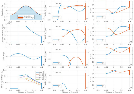
Figure 9.
Simplified breaker model. Left column: (a) a sketch of breaking wave profile, (d) standard deviation of breaker-induced surface elevation, (g) local normal angle, (j) mean-square slope of breaker-induced roughness. Middle column: up and downwave breaker NRCS for various incidence angles, (b) , (e) , (h) , (k) . Right column: up and downwave breaker effective Fresnel coefficient normalized by the nominal Fresnel coefficient, , for various incidence angles, (c) , (f) , (i) , (l) .
The GO approximation, Equation (9), is used to relate the simulated wave kinematics with the local breaker NRCS, , which now accounts for the spatial variations in local tilt and MSS:
where is the local incidence angle, is the local MSS of breaker-induced roughness component with wavenumbers, , (referred to as large scale breaker roughness), and is the effective Fresnel coefficient related to the nominal one, , as,
where is the short-scale (subgrid) breaker-induced height variance associated with wavenumbers greater than one third of the local Bragg wavenumber , . For the breaker spectrum, Equation (15), the short-scale surface variance and local MSS are,
The local normal zenith angle of the breaking surface is,
Thus, the local incidence angle, , is determined by the local normal, , radar incidence angle, , and the radar-to-wave azimuth, ,
Figure 9 illustrates an example of simulated breaker NRCS characteristics. In these calculations, the dimensionless tuning parameters of the model were specified as: (breaker life span) and (spatial decay rate).
Figure 9b demonstrates the distribution of breaker roughness variance along the breaking wave from the front slope, where the roughness is generated, towards the rear slope, where it attenuates and disappears, as imposed by the breaker life span.
The large-scale breaker MSS that accounts for breaker backscattering, Equation (24), depends on the incidence angle through the Bragg wavenumber and it decreases with (Figure 9d). The effective Fresnel coefficient, Equation (22), is sensitive to the short-scale roughness, especially in the Ka-band. Its typical value is , but it changes by a factor of 1 to 0.3, depending on and local breaker coordinate, x. Figure 9 (middle column) illustrates breaker NRCS distributions along breaking wave profiles for different observed in our experiments. Spike-like radar backscattering features are present near the forward and backward edges of a steep breaker due to sharp changes in the local incidence angle, . The relative contribution of these spike-like backscattering features and backscattering from the interior breaker roughness to the total breaker NRCS depends on . At large , the spike-like backscattering dominates.
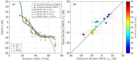
4.2. Comparison with the Measurements
In order to compare the simulated and observed breaker NRCS, the model equivalent of the measured breaker NRCS, Equation (13), needs to be defined. The model breaker NRCS averaged over the computantional domain (breaking wave wavelength), , (with being given by Equation (21)) is to be scaled by . Because, in the model , the model proxy for measured breaker NRCS reads,
The experimental estimates of the breaker NRCS defined by Equation (13) are shown in Figure 10a. The use of the sea surface fraction covered by enhanced breaker roughness as a scaling parameter in Equation (13) lowers the breaker NRCS by 2-3 dB in comparison with the whitecap coverage scaling, Equation (8). The simulated breaker NRCS values are consistent with observed values and they reproduce both the breaker NRCS magnitude and its dependence on . Except for the large , the model is virtually insensitive to the breaking wave wavelength for typical 1 to 10 m breaking waves observed in our experiments. Overall, good correspondence is found between the simulated and observed breaker NRCS values (Figure 10b).
5. Conclusions
In this work, the tower-based temporally synchronized and spatially collocated radar and video field measurements are used to estimate the normalized radar cross-section (NRCS) of breaking waves. The experiments were conducted in 2009–2013 from the Black sea stationary research platform while using Ka-band continuous-wave radar in a wide range of environmental conditions. During these experiments, the observed wind speed changed from 4 m/s to 16 m/s, with a 9 m/s median value, and the incidence angle varied from to .
Parts of radar records corresponding to breaking events are selected from optically-derived whitecap coverage fraction of the radar footprint, Q, as calculated from binarized video data. The detected breaking events, a total of ∼1000, are individually analyzed to provide various geometric characteristics of whitecaps, such as their length, area, speed, footprint fraction, and direction. If more than one breaking event occurs within the footprint, their geometric characteristics are computed as weighted-averages, with the weight proportional to individual breaker footprint fraction. The optically-derived geometric characteristics of whitecaps are compared with the synchronized radar data.
The contribution of whitecaps to the sea surface NRCS reflects in the increase of the polarization ratio (PR) and radar backscattering spikes, and it becomes distinguishable at . In our records, the observed Q was less than even for the largest breaking events. Thus, the contribution of the background backscattering from the regular, whitecap-free sea surface is not negligible.
Using the radar Doppler channel as a proxy for the modulating long wave orbital velocity, the background NRCS, polarization difference (PD), and polarization ratio (PR) are estimated as a function of the long wave phase. These characteristics are computed for whitecap-free and whitecap conditions by selecting the lower and upper percentiles of the radar footprint coverage, Q. These calculations reveal a clear contribution of whitecaps to the NRCS and PR, but not to the PD (as defined by the Bragg scattering), in turn suggesting a non-polarized backscattering mechanism from breaking waves.
Subtracting the whitecap-free background NRCS from the NRCS for whitecap-covered areas and using the measured Q, the whitecap backscattering contribution is evaluated. This quantity is found to be close to the only, to the best of our knowledge, calibrated NRCS measurements of laboratory foil-generated breaking waves that were described by Ericson et al. [35]. An interesting and unexpected feature is the negative, downwave > upwave, NRCS asymmetry observed at small incidence angles, .
A comparison of this paper whitecap NRCS estimates with the Geometric Optics (GO) model and GO-based parameterization of [10] shows a general consistency between the observed and model NRCS values. However, some features, including the incidence angle dependence and negative asymmetry at small are not reproduced by these models. To explain them, a modified GO-based model that accounts for breaker roughness variations along breaking wave profile is suggested.
Instead of optically-derived whitecap fraction, Q, we propose considering a more general variable referred to as breaker footprint fraction, q. This latter parameter is introduced to describe the whole breaking surface area (turnover) rather than only its visually-detectable part. Following the Phillips [51]-function concept, this q-area is proportional to the breaking crest length per unit surface area, , breaking wave phase speed, and active breaker lifetime. The breaker fraction, q, is larger than the whitecap fraction, Q, by 2–3 dB. It allows accounting for the whole breaking roughness and it is not limited to the bright foam pattern only.
A simplified, phenomenological 1-D model of breaker-induced backscattering that utilizes the Ericson et al. [35] breaker-induced roughness spectrum is proposed. The model is based on the geometric optics backscattering approximation and it has only one fitting parameter that accounts for the spatial scale of breaker decay. The model qualitatively agrees with the observed magnitude of breaker NRCS, its incidence angle dependence, and upwave/downwave asymmetry. The model-to-observation correspondence deteriorates at large incidence angles, . The approach employed to subtract the background backscattering may not be that accurate at these large incidence angles.
The contribution of wave breaking NRCS, , to the total radar NRCS, which is referred to as the non-polarized radar backscattering, NP, should account for all of the breaking wave scales
where is the spectral distribution of the breaking crest length per unit surface area [51], and is the breaker NRCS defined either empirically (Figure 10) or using a model. The simplified model that is proposed in Section 4.1 can be incorporated in radar imaging models that are suitable for real ocean conditions, where the NP contribution from breaking waves is significant, e.g., [6,10,43,53].
The complex and significant time and space evolution of the local breaker NRCS from a spike-like feature at the forward breaker front, which propagates with the phase velocity of a breaking wave, to the smooth breaker tail (that is embedded in the water and propagates with the orbital velocity), is expected to be among key factors governing the Doppler breaker signature. These hypotheses will guide our future research.
Supplementary Materials
The following are available online at https://www.mdpi.com/article/10.3390/rs13101929/s1, Video S1: Radar cross-section signatures of breaking waves.
Author Contributions
Y.Y.Y. and V.N.K. conceived and designed the experiments; V.N.K., S.A.G. and B.C. provided the electromagnetic modeling; Y.Y.Y. performed the experiments, analyzed the data, and wrote the paper. All authors have read and agreed to the published version of the manuscript.
Funding
The data analysis and wave breaking model development performed in this work were funded by the Russian Science Foundation under grant No. 21-47-00038. The field experiments were funded by the MHI RAS State Order (Goszadanie) No. 0555-2021-0004. Sea surface electromagnetic modeling was funded by the RSHU State Order (Goszadaine) No. 0763-2020-0005.
Institutional Review Board Statement
Not applicable.
Informed Consent Statement
Not applicable.
Conflicts of Interest
The authors declare no conflict of interest.
References
- Valenzuela, G.R. Theories for the interaction of electromagnetic and ocean waves—A review. Bound.-Layer Meteorol. 1978, 13, 61–85. [Google Scholar] [CrossRef]
- Elfouhaily, T.M.; Guérin, C.A. TOPICAL REVIEW: A critical survey of approximate scattering wave theories from random rough surfaces. Waves Random Media 2004, 14, 1. [Google Scholar] [CrossRef]
- Kanevsky, M.B. Radar Imaging of the Ocean Waves; Elsevier: Amsterdam, The Netherlands, 2009. [Google Scholar] [CrossRef]
- Chapron, B.; Kerbaol, V.; Vandemark, D.; Elfouhaily, T. Importance of peakedness in sea surface slope measurements and applications. J. Geophys. Res. Oceans 2000, 105, 17195–17202. [Google Scholar] [CrossRef]
- Chapron, B.; Johnsen, H.; Garello, R. Wave and wind retrieval from sar images of the ocean. Ann. Télécommun. 2001, 56, 682–699. [Google Scholar] [CrossRef]
- Voronovich, A.G.; Zavorotny, V.U. Theoretical model for scattering of radar signals in Ku- and C-bands from a rough sea surface with breaking waves. Waves Random Media 2001, 11, 247–269. [Google Scholar] [CrossRef]
- Chapron, B.; Vandemark, D.; Elfouhaily, T. On the skewness of the sea slope probability distribution. In Gas Transfer at Water Surface; Donelan, M.A., Drennan, W.M., Saltzman, E.S., Wanninkhof, R., Eds.; AGU: Washington, DC, USA, 2002; Volume 127, pp. 59–63. [Google Scholar] [CrossRef]
- Mouche, A.A.; Chapron, B.; Reul, N.; Hauser, D.; Quilfen, Y. Importance of the sea surface curvature to interpret the normalized radar cross section. J. Geophys. Res. Oceans 2007, 112, 10002. [Google Scholar] [CrossRef]
- Walsh, E.J.; Wright, C.W.; Banner, M.L.; Vandemark, D.C.; Chapron, B.; Jensen, J.; Lee, S. The Southern Ocean Waves Experiment. Part III: Sea Surface Slope Statistics and Near-Nadir Remote Sensing. J. Phys. Oceanogr. 2008, 38, 670–685. [Google Scholar] [CrossRef]
- Kudryavtsev, V.; Hauser, D.; Caudal, G.; Chapron, B. A semiempirical model of the normalized radar cross-section of the sea surface 1. Background model. J. Geophys. Res. Oceans 2003, 108, FET 2-1–FET 2-24. [Google Scholar] [CrossRef]
- Hansen, M.W.; Kudryavtsev, V.; Chapron, B.; Johannessen, J.A.; Collard, F.; Dagestad, K.F.; Mouche, A.A. Simulation of radar backscatter and Doppler shifts of wave-current interaction in the presence of strong tidal current. Remote Sens. Environ. 2012, 120, 113–122. [Google Scholar] [CrossRef]
- Kalmykov, A.I.; Pustovoytenko, V.V. On polarization features of radio signals scattered from the sea surface at small grazing angles. J. Geophys. Res. 1976, 81, 1960–1964. [Google Scholar] [CrossRef]
- Plant, W.J. The Modulation Transfer Function: Concept and Applications. In Radar Scattering from Modulated Wind Waves; Komen, G.J., Oost, W.A., Eds.; Springer: Dordrecht, The Netherlands, 1989; pp. 155–172. [Google Scholar] [CrossRef]
- Keller, W.C.; Plant, W.J.; Petitt, R.A.; Terray, E.A. Microwave backscatter from the sea: Modulation of received power and Doppler bandwidth by long waves. J. Geophys. Res. Oceans 1994, 99, 9751–9766. [Google Scholar] [CrossRef]
- Kudryavtsev, V.; Hauser, D.; Caudal, G.; Chapron, B. A semiempirical model of the normalized radar cross section of the sea surface, 2. Radar modulation transfer function. J. Geophys. Res. Oceans 2003, 108, FET 3-1–FET 3-16. [Google Scholar] [CrossRef]
- Hwang, P.A.; Sletten, M.A.; Toporkov, J.V. Breaking wave contribution to low grazing angle radar backscatter from the ocean surface. J. Geophys. Res. Oceans 2008, 113. [Google Scholar] [CrossRef]
- Malinovsky, V.V.; Korinenko, A.E.; Kudryavtsev, V.N. Empirical Model of Radar Scattering in the 3-cm Wavelength Range on the Sea at Wide Incidence Angles. Radiophys. Quantum Electron. 2018, 61, 98–108. [Google Scholar] [CrossRef]
- Kudryavtsev, V.N.; Chapron, B.; Myasoedov, A.G.; Collard, F.; Johannessen, J.A. On Dual Co-Polarized SAR Measurements of the Ocean Surface. IEEE Geosci. Remote Sens. Lett. 2013, 10, 761–765. [Google Scholar] [CrossRef]
- Kudryavtsev, V.; Kozlov, I.; Chapron, B.; Johannessen, J.A. Quad-polarization SAR features of ocean currents. J. Geophys. Res. Oceans 2014, 119, 6046–6065. [Google Scholar] [CrossRef]
- Hansen, M.W.; Kudryavtsev, V.; Chapron, B.; Brekke, C.; Johannessen, J.A. Wave Breaking in Slicks: Impacts on C-Band Quad-Polarized SAR Measurements. IEEE J. Sel. Top. Appl. Earth Obs. Remote Sens. 2016, 9, 4929–4940. [Google Scholar] [CrossRef]
- Kudryavtsev, V.N.; Fan, S.; Zhang, B.; Mouche, A.A.; Chapron, B. On Quad-Polarized SAR Measurements of the Ocean Surface. IEEE Trans. Geosci. Remote Sens. 2019, 57, 8362–8370. [Google Scholar] [CrossRef]
- Zhang, B.; Zhao, X.; Perrie, W.; Kudryavtsev, V. On Modeling of Quad-Polarization Radar Scattering from the Ocean Surface with Breaking Waves. J. Geophys. Res. Oceans 2020, 125, e2020JC016319. [Google Scholar] [CrossRef]
- Lewis, B.L.; Olin, I.D. Experimental study and theoretical model of high-resolution radar backscatter from the sea. Radio Sci. 1980, 15, 815–828. [Google Scholar] [CrossRef]
- Jessup, A.T.; Keller, W.C.; Melville, W.K. Measurements of sea spikes in microwave backscatter at moderate incidence. J. Geophys. Res. Oceans 1990, 95, 9679–9688. [Google Scholar] [CrossRef]
- Jessup, A.T.; Melville, W.K.; Keller, W.C. Breaking waves affecting microwave backscatter 1. Detection and verification. J. Geophys. Res. Oceans 1991, 96, 20547–20559. [Google Scholar] [CrossRef]
- Jessup, A.T.; Melville, W.K.; Keller, W.C. Breaking waves affecting microwave backscatter 2. Dependence on wind and wave conditions. J. Geophys. Res. Oceans 1991, 96, 20561–20569. [Google Scholar] [CrossRef]
- Lee, P.H.Y.; Barter, J.D.; Beach, K.L.; Hindman, C.L.; Lake, B.M.; Rungaldier, H.; Shelton, J.C.; Williams, A.B.; Yee, R.; Yuen, H.C. X band microwave backscattering from ocean waves. J. Geophys. Res. 1995, 100, 2591–2612. [Google Scholar] [CrossRef]
- Liu, Y.; Frasier, S.J.; McIntosh, R.E. Measurement and classification of low-grazing-angle radar sea spikes. IEEE Trans. Antennas Propag. 1998, 46, 27–40. [Google Scholar] [CrossRef]
- Ermakov, S.A.; Kapustin, I.A.; Kudryavtsev, V.N.; Sergievskaya, I.A.; Shomina, O.V.; Chapron, B.; Yurovskiy, Y.Y. On the Doppler Frequency Shifts of Radar Signals Backscattered from the Sea Surface. Radiophys. Quantum Electron. 2014, 57, 239–250. [Google Scholar] [CrossRef]
- Ermakov, S.A.; Dobrokhotov, V.A.; Sergievskaya, I.A.; Kapustin, I.A. Suppression of Wind Ripples and Microwave Backscattering Due to Turbulence Generated by Breaking Surface Waves. Remote Sens. 2020, 12, 3618. [Google Scholar] [CrossRef]
- Kwoh, D.S.W.; Lake, B.M. A Deterministic, Coherent, and Dual-Polarized Laboratory Study of Microwave Backscattering From Water Waves, Part 1: Short Gravity Waves Without Wind. IEEE J. Oceanic Eng. 1984, 9, 291–308. [Google Scholar] [CrossRef]
- Lamont-Smith, T.; Waseda, T.; Rheem, C.K. Measurements of the Doppler spectra of breaking waves. IET Radar Sonar Navig. 2007, 1, 149–157. [Google Scholar] [CrossRef]
- Lee, P.H.Y.; Barter, J.D.; Beach, K.L.; Lake, B.M.; Rungaldier, H.; Thompson, H.R.; Yee, R. Scattering from breaking gravity waves without wind. IEEE Trans. Antennas Propag. 1998, 46, 14–26. [Google Scholar] [CrossRef]
- Fedorov, A.V.; Melville, W.K.; Rozenberg, A. An experimental and numerical study of parasitic capillary waves. Phys. Fluids 1998, 10, 1315–1323. [Google Scholar] [CrossRef]
- Ericson, E.A.; Lyzenga, D.R.; Walker, D.T. Radar backscattering from stationary breaking waves. J. Geophys. Res. Oceans 1999, 104, 29679–29695. [Google Scholar] [CrossRef]
- Fuchs, J.; Regas, D.; Waseda, T.; Welch, S.; Tulin, M.P. Correlation of hydrodynamic features with LGA radar backscatter from breaking waves. IEEE Trans. Geosci. Remote Sens. 1999, 37, 2442–2460. [Google Scholar] [CrossRef]
- Walker, D. Experimentally motivated model for low grazing angle radar Doppler spectra of the sea surface. IEE Proc.-Radar Sonar Navig. 2000, 147, 114–120. [Google Scholar] [CrossRef]
- Dano, E.B.; Lyzenga, D.R.; Perlin, M. Radar Backscattering from Mechanically Generated Transient Breaking Waves—Part 1: Angle of Incidence Dependence and High Resolution Surface Morphology. IEEE J. Oceanic Eng. 2001, 26, 181–200. [Google Scholar] [CrossRef]
- Dano, E.B.; Lyzenga, D.R.; Meadows, G.; Meadows, L.; van Sumeren, H.; Onstott, R. Radar Backscattering from Mechanically Generated Transient Breaking Waves—Part 2: Azimuthal and Grazing Angle Dependence. IEEE J. Oceanic Eng. 2001, 26, 201–215. [Google Scholar] [CrossRef]
- Rozenberg, A.; Ritter, M. Laboratory study of the fine structure of short surface waves due to breaking: Two-directional wave propagation. J. Geophys. Res. Oceans 2005, 110. [Google Scholar] [CrossRef]
- Ermakov, S.A.; Kapustin, I.A.; Sergievskaya, I.A. Tank study of radar backscattering from strongly nonlinear water waves. Bull. Russ. Acad. Sci. Phys. 2010, 74, 1695–1698. [Google Scholar] [CrossRef]
- Rodriguez, E. On the Optimal Design of Doppler Scatterometers. Remote Sens. 2018, 10, 1765. [Google Scholar] [CrossRef]
- Yurovsky, Y.Y.; Kudryavtsev, V.N.; Grodsky, S.A.; Chapron, B. Ka-Band Dual Copolarized Empirical Model for the Sea Surface Radar Cross Section. IEEE Trans. Geosci. Remote Sens. 2016, 55, 1629–1647. [Google Scholar] [CrossRef]
- Yurovsky, Y.Y.; Kudryavtsev, V.N.; Chapron, B.; Grodsky, S.A. Modulation of Ka-band Doppler Radar Signals Backscattered from the Sea Surface. IEEE Trans. Geosci. Remote Sens. 2018, 56, 2931–2948. [Google Scholar] [CrossRef]
- Yurovsky, Y.Y.; Kudryavtsev, V.N.; Grodsky, S.A.; Chapron, B. Low-Frequency Sea Surface Radar Doppler Echo. Remote Sens. 2018, 10, 870. [Google Scholar] [CrossRef]
- Yurovsky, Y.Y.; Kudryavtsev, V.N.; Grodsky, S.A.; Chapron, B. Sea Surface Ka-Band Doppler Measurements: Analysis and Model Development. Remote Sens. 2019, 11, 839. [Google Scholar] [CrossRef]
- Monahan, E.C.; Woolf, D.K. Comments on “Variations of Whitecap Coverage with Wind stress and Water Temperature. J. Phys. Oceanogr. 1989, 19, 706–709. [Google Scholar] [CrossRef]
- Bondur, V.G.; Sharkov, E.A. Statistical Characteristics of Foam Formations on a Disturbed Sea-surface. Okeanologiya 1982, 22, 372–379. [Google Scholar]
- Gonzalez, R.C.; Woods, R.E.; Eddins, S.L. Digital Image Processing Using MATLAB; Gatesmark Publishing: Knoxville, TN, USA, 2009. [Google Scholar]
- Yurovsky, Y.Y.; Kudryavtsev, V.N.; Chapron, B.; Grodsky, S.A. How Fast are Fast Scatterers Associated with Breaking Wind Waves? In Proceedings of the IGARSS 2018—2018 IEEE International Geoscience and Remote Sensing Symposium, Valencia, Spain, 22–27 July 2018; pp. 142–145. [Google Scholar] [CrossRef]
- Phillips, O.M. Radar returns from the sea surface—Bragg scattering and breaking waves. J. Phys. Oceanogr. 1988, 18, 1065–1074. [Google Scholar] [CrossRef]
- Korinenko, A.E.; Malinovsky, V.V.; Kudryavtsev, V.N. Experimental Research of Statistical Characteristics of Wind Wave Breaking. Phys. Oceanogr. 2018, 25, 489–500. [Google Scholar] [CrossRef][Green Version]
- Hwang, P.A.; Sletten, M.A.; Toporkov, J.V. Analysis of radar sea return for breaking wave investigation. J. Geophys. Res. Oceans 2008, 113. [Google Scholar] [CrossRef]


Publisher’s Note: MDPI stays neutral with regard to jurisdictional claims in published maps and institutional affiliations. |
© 2021 by the authors. Licensee MDPI, Basel, Switzerland. This article is an open access article distributed under the terms and conditions of the Creative Commons Attribution (CC BY) license (https://creativecommons.org/licenses/by/4.0/).