Abstract
The use and research of Unmanned Aerial Vehicle (UAV) have been increasing over the years due to the applicability in several operations such as search and rescue, delivery, surveillance, and others. Considering the increased presence of these vehicles in the airspace, it becomes necessary to reflect on the safety issues or failures that the UAVs may have and the appropriate action. Moreover, in many missions, the vehicle will not return to its original location. If it fails to arrive at the landing spot, it needs to have the onboard capability to estimate the best area to safely land. This paper addresses the scenario of detecting a safe landing spot during operation. The algorithm classifies the incoming Light Detection and Ranging (LiDAR) data and store the location of suitable areas. The developed method analyses geometric features on point cloud data and detects potential right spots. The algorithm uses the Principal Component Analysis (PCA) to find planes in point cloud clusters. The areas that have a slope less than a threshold are considered potential landing spots. These spots are evaluated regarding ground and vehicle conditions such as the distance to the UAV, the presence of obstacles, the area’s roughness, and the spot’s slope. Finally, the output of the algorithm is the optimum spot to land and can vary during operation. The proposed approach evaluates the algorithm in simulated scenarios and an experimental dataset presenting suitability to be applied in real-time operations.
1. Introduction
Presently, Unmanned Aerial Vehicles (UAVs) are gaining more interest in the scientific and industrial research community due to their autonomy, maneuverability, and payload capacity, making them suitable robots to perform real-world tasks in different scenarios. There have been several research topics related to hardware development, human-system interaction, obstacle detection, and collision avoidance [1]. The UAVs are designed to be remotely controlled by a human operator or execute a mission autonomously [2]. In the latter case, the degree of autonomy and the mission they can achieve depends on the sensors used. Concerning the UAV classification, there are several ways in which UAVs can be defined: aerodynamics, landing, weight, and range [3]. Considering the state of the art of UAVs, commercial or research, there is a large spectrum of applications, such as search-and-rescue operations [4,5], delivery, surveillance, inspection, and interaction with the environment [6,7].
Given the application scenarios, there are missions where the UAV must fly in civilian airspace; i.e., they must fly over populated areas. However, they are susceptible to external disturbance or electromechanical malfunction. Different failure scenarios could impact the operation, thus leading to an emergency landing:
- Global Positioning System (GPS) failures. In general, UAVs use GPS messages to navigate. Although several sensors could aid the navigation, the vehicle may need to land in the occurrence of loss of GPS signal.
- Loss of communication. In the event of loss of communication between the UAV and a base station, one possible action is to perform an emergency landing.
- Battery failure. If a battery failure is detected, the vehicle may not be able to continue its operation, and as a result, an emergency landing is necessary.
- Software and hardware errors. A UAV can experience a mechanical fault during a mission, like a broken propeller or a fail in the motor, or even a software issue that could require that the vehicle must perform an emergency landing.
- Environment factors. Bad weather conditions such as strong winds and rain make the vehicle unable to carry out the mission, forcing it to land.
In these situation, UAVs must safely land to reduce damage to themselves and avoid causing any injury to humans.
Consequently, detecting a reliable landing spot is essential to safe operation. In order to estimate a landing spot, a set of conditions must be evaluated when analyzing the sensor data. These conditions are typically restraints on the landing surface. The reliability of a safe landing site depends on several factors, such as the aircraft’s distance to the landing site and the ground conditions, such as (a) the slope of the plane: the landing spot must have a slope smaller than a threshold so that the vehicle does not slide when landing; (b) the roughness of the area: there are cases when the vehicle will land on a surface with vegetation or other small obstacles—in this case, these obstacles’ height must not be larger than a maximum value predefined before the mission, avoiding contact with the propellers; (c) the size of the spot: the landing spot must be large enough for the UAV; (d) the presence of obstacles: the approximation to landing spot depends on the area’s obstacles, namely building, vegetation, or humans. Therefore, the presence of obstacles must be taken into account when evaluating the spot. Another rule also imposed on the algorithm is the distance to the landing spot. The UAV must be able to reach the desired spot with the remaining battery power. Since one factor is the aircraft’s distance to the landing site, the landing spot’s suitability varies during the mission. Figure 1 illustrates the conceptual approach for emergency landing spot detection with a UAV in real-time.
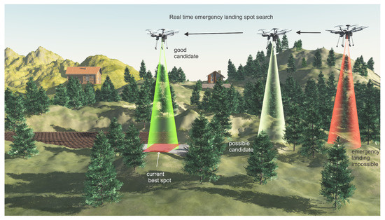
Figure 1.
Conceptual approach for emergency landing spot detection with a UAV.
Considering the robustness problems that a UAV faces during an autonomous mission, this paper addresses developing an algorithm for detecting, storing, and selecting real-time emergency landing spots based on LiDAR data. The main focus is to develop an algorithm that will continuously evaluate the terrain based on LiDAR data and establish a list of possible landing spots. Additionally, a continuous evaluation of the detected landing spots is required given that the best spot can vary during the UAV operation. The developed algorithm accumulates the 3D point cloud provided by the sensor and then generates downsampled point clouds. Following that, a plane is detected by applying the PCA algorithm in a spherical neighborhood. The potential spots are subsequently evaluated regarding different parameters, and finally, the resulting score is assigned to the spot. This paper is an extended version of work published in [8,9]. Compared to the previous papers [8,9], this work presents a more extensive review of the related works. Furthermore, the proposed approach was evaluated with field tests during a 3D reconstruction survey mission that took place in the Monastery of Tibães, Braga, Portugal. The results were also improved with the evaluation of spots’ score for each dataset. This work intends to contribute by applying a Voxel Grid Filter to the point clouds provided by a LiDAR. The application of this filter speeds up the plane detection step by reducing the size of the point cloud and removing redundant points. Moreover, it is shown that the algorithm can obtain a list of safe landing spots without segmenting the entire point cloud by analyzing spherical regions within it.
The paper outline is as follows: Section 2 presents a preliminary study of the related works regarding emergency landing and landing detection given LiDAR and camera data. Then, Section 3 shows the high-level hardware and software architecture, detailing their components. Section 4 introduces the developed algorithm and its requirements. In addition, the algorithm sequence of data processing blocks is displayed and explained. In Section 5, the results obtained are presented, as well as the analyses and performance of the algorithm. Finally, in Section 7, we discuss the conclusions of the method for detecting safe landing spots. Here we also present suggestions or directions for further work.
2. Related Work
The main problem to be addressed is the integration in a UAV to detect safe landing zones. Thus, it is necessary to process different types of data from several sensors so that it is possible to obtain information about the surface where we intended to land. Each sensor onboard the UAV provides specific information regarding terrain and obstacles and therefore has advantages and disadvantages that must be evaluated. Consequently, there are multiple literature approaches regarding safe landing, either for emergencies or for other purposes.
2.1. LiDAR Based Detection Systems
Among the primary sensors used to solve the problem of detecting emergency landing spots is LiDAR. Generally, the point clouds are processed, determining terrain features such as slope and roughness. In addition, LiDAR data present usefulness in other tasks, for instance, hazard detection and avoidance. Typically, a geometric approach is a common approach concerning LiDAR data.
In 2002, in order to perceive obstacles and land spacecraft, a 2.5D grid map technique was used by Johnson et al. [10]. Their work applied a Least Mean Square (LMS) algorithm to estimate a plane in the grid map, computing the incidence angle and the roughness to generate a landing cost map. Another geometric approach was presented by Whalley et al. [11,12] in 2009. In the author’s strategy, each LiDAR scan is mapped to a grid in which a sliding window moves along to calculate the terrain restraints. Finally, the optimal spot is chosen after the entire grid is covered.
Regarding unknown environments, Chamberlain et al. [13], in 2011, presented a proposal that permits a full-scale unmanned helicopter to land without human control or input. Their methodology utilizes a 3D scanning LiDAR in two modes. A forward scan is performed to detect obstacles, and a downward scan is subsequently carried out to map the environment. A 3D virtual model of the helicopter is placed on each cell of the resulting map. An assessment of the area is executed considering the skid contact, wind direction, and presence of obstacles. This work is expanded in [14,15,16] by presenting experimental results in urban and natural environments. In the evaluation step, a 2D Delaunay triangulation [17] of the potential landing sites data is generated in order to establish the intersections with the landing skids and the roll and pitch of the helicopter. Ultimately, the volume between the triangulation and the 3D model is used to estimate bad contact.
One of the drawbacks of the geometric approach is the presence of low vegetation in the landing spot, as it makes the spot extremely rough. In order to overcome this hindrance, Maturana and Scherer [18] proposed a 3D Convolutional Neural Network [19] algorithm. The strategy is to generate a volumetric density map given the globally registered LiDAR point clouds. The volumetric map is then divided into sub-volumes that are the input of the neural network. The algorithm was able to detect small obstacles using synthetic datasets and simulation.
In 2017, Lorenzo et al. [20] proposed a landing site detection algorithm on many core systems by using parallel processing. An octree is built in order to increase process speed during a neighborhood search step. Then, the normal of all points are computed in parallel, and geometric restraints are used to assess the spot.
Recently, the authors of [21] proposed an approach to select landing zones based on a region growing algorithm. The initial strategy is to find flat regions from LiDAR point clouds and then apply a Progressive Sample Consensus (PROSAC) algorithm to fit a plane. The detected planes are assessed conforming slope, roughness and maximum difference of height. However, the proposed method was only evaluated in simulation experiments and the PROSAC algorithm can be time consuming.
2.2. Vision-Based Detection Systems
The vision-based system has been the most popular approach to detect and evaluate a landing spot. There are multiple strategies to land a UAV using vision-based algorithms. Cameras have the advantage of being inexpensive and lighter compared to LiDARs. Bosch et al. [22] developed an algorithm to autonomously detect landing sites with monocular images. First, a cluster of potential points in a plane is selected by applying a homography estimation process. Then, the algorithm distinguishes planar from non-planar surfaces. This information is stored in the stochastic 2D grid cell. However, this proposal stores the probability of the region being flat and hence cannot be used for other applications, such as obstacle avoidance.
Several works have used machine vision to detect landing spots [23,24,25]. The authors proposed a technique that generates two binary images by applying a Canny Edge Detector and a line-expansion algorithm. Given the fusion of the two images, the preliminary map is built to label safe and unsafe areas. Then, the surface is classified, and fuzzy logic is used to select the safest spot. The work was later expanded in 2015 by Warren et al. [26]. A 3D reconstruction using Structure-from-Motion is carried out to analyze the surface.
Eendebak et al. [27] presented a technique for emergency landing in real-time operations given camera movement. Their work is based on a Background Estimation on stabilized video in which the camera frames are compared to distinguish moving objects and structures. Then, a distance map to all detected obstacles is generated. The maximum distance on the map is calculated and chosen as the best landing area.
Forster et al. [28] proposed an elevation map-based technique to landing spot detection for micro-aerial vehicles using a monocular camera. A depth map is generated given the camera images and the vehicle’s pose. Furthermore, an elevation map is also built and consequently updated according to the depth maps. During the algorithm selection stage, a flat surface with a radius depending on the vehicle size is considered a landing spot.
Another proposal to detect landing spots in unknown environments in real-time is presented by Hinzmann et al. [29]. A segmentation step is applied to the camera images, classifying the regions as “grass” or “not grass.” Next, 3D reconstruction and elevation maps are achieved given the results of the segmentation stage. Finally, the area is assessed considering the ground features, such as slope and roughness.
In 2019, Kaljahi et al. [30] proposed a system for detecting landing sites using Gabor Transform and Markov chain codes. The authors proposed a method that obtains flat surfaces from images using the Gabor Transform. Then, histogram operations are applied in order to determine the pixels that contribute to the highest peak. The next step consists of using Markov Chain Codes to estimate and group potential pixels as candidate regions. For each candidate region, Chi square distance is computed and compared to a reference to define the similarity between the regions, resulting in the final safe landing zone.
In 2020, Bektash et al. [31] presented a machine-vision-based algorithm to recognize landing areas. The model chosen for the network was the convolutional neural network that receives split images provided by a camera as an input. However, manual vision inspection of the camera frames is used as criteria for classifying the landing site.
2.3. Other Approaches
In addition to techniques that use one primary sensor to solve landing detection, other approaches combine multiple sources of information. Serrano [32] presented a probabilistic framework using Radio Detection Furthermore, Ranging (RADAR), LiDAR, and camera data to improve the robustness of the selection of landing sites stage in space operation. By applying a Least Median of Squares regression to fit a plane using the RADAR and LiDAR data, the authors calculated the terrain slope and roughness. Furthermore, an edge detection algorithm is applied in the camera images to distinguish craters and rocks. Finally, a Bayesian Network [33] is used to evaluate the area safety considering the information acquired in the previous steps.
Using a similar set of sensors, Howard and Seraji [34] built three hazard maps from RADAR, LiDAR, and camera data. These maps were then used to obtain measurements and the landing site features in which each map is labeled with a confidence variable. Finally, the maps were fused using fuzzy logic presenting the landing site safety.
2.4. Overall Discussion
The decision between LiDARs or cameras to serve as the primary sensor to detect emergency landing spots depends on the vehicle’s characteristics and the mission in which it will be applied. Generally, the feasibility of vision-based techniques depends on visibility restrictions. However, this drawback can be easily overcome by LiDARs sensors. Nevertheless, the processing power, weight, and price of LiDARs are more demanding for UAVs than cameras.
The use of LiDAR is justified due to the greater robustness to situations of luminosity variations [14,15,21], already obtaining depth information at the instant of the SCAN, not requiring a stereo baseline or depth estimation by sequence of images, and being robust in flights nocturnal.
In terms of processing time of LiDAR-based systems, the current works indicate the importance of knowing the sensor data structure to reduce the number of operations and, thereby, to improve data access efficiency and execution time of the algorithm. Hence, the point clouds are generally spatially structured. It is worth noting that the approach chosen for structuring can cause loss of spatial information, such as 2.5D grid and plane-projected images. Consequently, additional statistical data must be stored in these scenarios.
Most of the works related to landing spots detection identify the terrain’s geometric features to find planar surfaces [10,11,12,13,14,15,16]. In general, the features are slope and roughness. Other approaches consist of neural networks or machine vision [18,23,24,25]. However, these techniques present the need to train the algorithm.
Regarding the selection of landing spots, the exposed works revealed the importance of classifying the area in a probabilistic manner. These probabilistic values should consider the possibility of landing, presence of obstructions, battery power, ground restraints. Consequently, the levels vary during the operation.
3. System Design
This section describes the hardware and software architectures that were considered during the implementation of the proposed algorithm. The landing spot detection algorithm was developed in Robotic Operating System (ROS) [35], due to providing a modular structure able to integrate available ROS packages straightforwardly with other software modules already available in the UAV.
The proposed framework processes the 3D point clouds provided by a LiDAR to detect landing zones in real time. Furthermore, another layer of software is responsible for analyzing the UAV status, such as remaining battery power, the status of hardware and software components. Therefore, in a failure situation in which a forced landing is necessary, this layer will search for the current best landing spot detected by the proposed algorithm.
3.1. Hardware
The landing spot detection algorithm is designed to be executed simultaneously with other UAV tasks during operation. The VLP-16 LiDAR provides 3D point clouds that are processed using an onboard computer. Considering that modern LiDARs produce hundreds of thousands of points in each scan, a high transmission rate between the sensor and the computer is necessary (Figure 2 in blue).
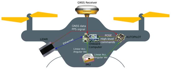
Figure 2.
High-level hardware architecture (adapted from Refs. [37,38]).
The point clouds are given in the LiDAR reference frame. Consequently, knowing the UAV pose is essential to transform the data to a fixed frame. There are several approaches to estimate the vehicle pose. In this case, the method is to fuse the Global Navigation Satellite System (GNSS) and Inertial Measurement Unit (IMU) measurements. Another critical issue is to correlate in real-time the LiDAR scan with all the UAV onboard sensors. Therefore, to ensure synchronization, the timestamp data from the GNSS is provided to both systems, LiDAR and PC, with Chrony [36] service.
3.2. Software
Figure 3 presents the high-level software architecture to detect a potential landing spot given a point cloud generated by a LiDAR sensor. All the pipeline elements were developed within the ROS framework, except for the sensor’s input data. The software is divided into several data processing-blocks:
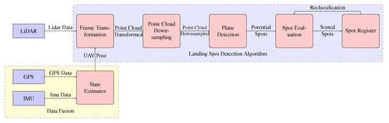
Figure 3.
High-level software pipeline.
- Data Fusion: the data fusion section estimates the UAV’s states by fusing the measurements from the IMU and GPS. There are several approaches to realize this procedure. For instance, an Extended Kalman Filter (EKF) can be applied.
- Frame Transformations: considering that the LiDAR is fixed to the vehicle, the LiDAR pose is correlated to the UAV pose. Therefore, the LiDAR point cloud can be transformed from the LiDAR frame to the local navigation frame. Using the tf2 (http://wiki.ros.org/tf2 (accessed on 14 May 2021)) package, the relations between the UAV, LiDAR and global coordinate frames are established.
- Point Cloud Downsampling: each LiDAR scan produces a point cloud with thousands of points. Considering that the vehicle did not travel a large distance to detect a spot, it is important to accumulate the point clouds in order to not to lose information. Conversely, accumulating the point clouds increases computational effort. Therefore, the referenced point cloud is downsampled.
- Plane Detection: following the downsampling of a point cloud, a plane can be detected in the new point cloud. The plane detection can be subdivided into several steps, confirming the available time, the computational power, and the desired resolution. Generally, the algorithms consist of estimating the parameters from the plane equation in a limited region of the original point cloud. Moreover, the algorithms have to fit a plane in the presence of outliers, i.e., points that do not fit the plane model. Besides the landing spot detection for aerial vehicles, estimating the ground conditions is also useful for detecting clear paths and making further processing less complex.
- Spot Evaluation: the segmented point cloud containing the detected plane is then evaluated to classify the spot’s reliability. The roughness of the landing zone can be assessed by computing the standard deviation in the z-axis. The higher the standard deviation, the rougher the area. In addition, a high value can also indicate the presence of obstacles, such as trees or buildings. The spots are also evaluated regarding their slope as the landing zone cannot be steep enough to destabilize the vehicle when landed. Furthermore, the size of the area and the distance to the UAV can also be used to evaluate the spot. Each evaluation factor has different importance according to the environment. Thus, it becomes interesting to assign different weights to these factors.
- Spot Register: the assessed spots are then registered as a landing spot. However, the suitability of a landing point to be the optimal choice varies during operation. In this way, the points registered have to be periodically reassessed.
4. Emergency Landing Spot Detection Algorithm
The developed algorithm procedure is divided into several steps: the frame transformation of the input data, the downsampling of the point cloud, the spatial structuring of the data, detection of planes, filtering of potential candidates, and classification of detected spots. In addition, there are some rules created to obtain the desired objective. Figure 4 shows the flowchart of the developed software.
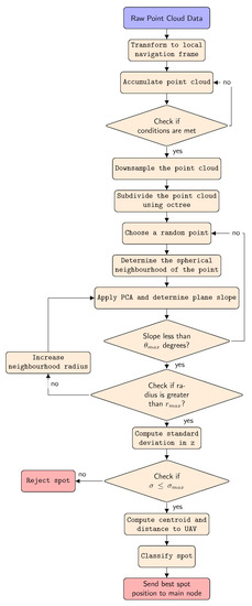
Figure 4.
Flowchart of the developed algorithm.
4.1. Frames Transformation
The pose of a robot is generally given in the local navigation coordinates system. Consequently, the landing spot must be in the same frame. However, LiDARs report data in their own reference frame. Then, the first step of our proposal is to transform the point cloud from the LiDAR reference frame to the local navigation reference frame. This procedure can be fulfilled by using transformation matrices. Therefore, the relation between the frames is defined by Equation (1):
Considering a 3D point in the LiDAR reference frame, at instant t, the transformation matrix given by transforms the point to the body reference frame. At this step, it is considered that the LiDAR is fixed to the robot, hence the matrix not varying over time. Finally, the matrix multiplied by results in the data expressed in the local navigation reference frame.
The algorithm does not apply the landing zone detection step for each LiDAR scan. This is due to the following reasons: the vehicle may not have traveled a sufficient distance to need a new spot other than the take off point; in addition, the sensor may not return sufficient points of the environment. Therefore, the point cloud registered in the local frame is stored until it reaches the conditions to start the next step. The defined conditions are:
- Traveled distance: if the robot has traveled a long distance in relation to the last landing spot, it becomes necessary to find a new location, since, in an emergency scenario, the vehicle may not be able to reach the landing zone.
- Size of accumulated point cloud: a high number of points in the point cloud increases the execution time of search algorithms and the memory consumption of the onboard computer. For this reason, if the size of the accumulated cloud reaches a threshold, the algorithm starts the next step.
At the moment, this step is done considering only the vehicle pose. However, in future projects, it is worth considering the vehicle velocity.
4.2. Point Cloud Downsampling
Accumulating the data until one of the necessary conditions are reached will increase the processing effort. In order to obtain better performance in terms of execution time and memory consumption, it becomes necessary to perform the downsampling of the point cloud. Therefore, a Voxel Grid filter [39] is applied. The filter takes a spatial average of the points in the cloud. A set of 3D volumetric pixels (voxel) grid with size is generated over the cloud, and the points are approximated with their centroid.
Figure 5 shows the result of the downsampling. At first analysis, the point clouds displayed in Figure 5a,b are almost identical. However, the downsample technique created a point cloud three times smaller in size. This method allows decreasing the number of points of the cloud and gives a point cloud with approximately constant density. Finally, the algorithm resets the original point cloud in order to free the memory.
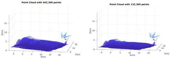
Figure 5.
Point cloud downsampling.
4.3. Data Structuring and Neighbor Search
The next step is to determine the neighborhood of a point to perform the plane identification method. The process of detecting a plane in a point cloud is the most time-consuming process in the algorithm. Due to the large number of data, this step needs to be optimized in order to obtain a real-time analysis. For this reason, the point cloud is spatially structured using octree [40]. Each internal node of the octree is subdivided into eight octants. By using a tree structure like an octree, the execution time of a search algorithm is considerably reduced [41]. There are several approaches to identify the neighborhood of a point. In this case, the algorithm finds the spherical neighborhood of a randomly chosen point. Considering a point in the point cloud, the neighborhood N(p) of this point with radius r is determined by:
where is any point in the cloud.
The minimum radius () of a plane is defined by the user as depends on sensor and environment characteristics. By applying Equation (2), all the points placed inside the sphere are considered as part of the neighborhood.
4.4. Plane Detection
After the previous step, it is possible to calculate a planar surface given the neighborhood points. This is done satisfactorily by using the PCA algorithm. PCA applies an orthogonal transformation to map the data to a set of values called principal components that correspond to the eigenvectors of the covariance matrix.
Considering the plane equation given by:
The normal vector is represented by:
The eigenvectors determined with PCA serve as the three axes of the plane while the eigenvalues indicate the square sum of points deviations along the corresponding axis. Therefore, the eigenvector with the smallest eigenvalue represents the normal vector given by Equation (4), and the points are bounded by the other two axes. In this perspective, the slope of the plane is examined using the normal vector. The slope is the angle between the normal vector and the vertical vector and is computed using Equation (5):
Hence, a first evaluation can be done using the plane slope. If the resulting value is greater than the maximum slope () permitted for the robot, the plane is rejected. Otherwise, the neighborhood radius used in the previous section is increased and the process is repeated until the maximum radius () is reached. By doing this procedure, the method tries to find regions with different sizes that can be considered a landing spot. Algorithm 1 describes the neighborhood and plane identification steps. The idea of the method is to detect planes for random search points with increasing radius. The PCA step is only performed if the number of points within the neighborhood sphere is greater than . The slope angle is immediately computed after detecting the plane and, if it is greater than , the plane is rejected and the algorithm restarts the process for a new search point. In addition, when we increase the radius of the sphere and a previously detected plane has a slope greater than the threshold, only the point cloud corresponding to the previous slope and the respective radius of the sphere is sent to the evaluation step.
| Algorithm 1 Algorithm for neighborhood and plane identification steps. |
| Input: pointcloud downsampled |
| Output: point cloud cluster |
|
In summary, only the planes that have a slope less than or equal to are sent to the register stage. Table 1 describes the parameters used in the algorithm.

Table 1.
The parameters used in the plane detection step.
4.5. Registration and Classification
Given the algorithm presented in the previous section, the next step consists in evaluating the detected planes. In this context, many factors are considered to decide the best landing spot. Initially, the point cloud centroid is computed and is considered the spot center. After this, each factor is computed individually. A score () from 0 to 20 is computed for each parameter. It is worth noting that the degree of importance for each parameter depends on the operation. Consequently, each grade has a different weight previously defined by the user. Finally, each spot is classified regarding the following equation:
Table 2 shows the parameters computed to classify the plane and their respective weights. In this stage, the planes that have standard deviation in the z-axis greater than the maximum standard deviation are immediately rejected.
Table 2.
The parameters that are analyzed to classify the spot.
Using these parameters, the algorithm evaluates the landing spot in terms of terrain roughness, vehicle stability when landed, obstacle clearance of a location and distance to the UAV. Ultimately, the spots are stored and sorted from highest rate to smallest. In general, a spot quality depends on the vehicle trajectory. In this perspective, the stored spots are re-evaluated periodically.
4.6. Algorithm Output
The algorithm returns the current best landing spot in the local navigation frame and the score obtained in the classification step. Concurrently, the algorithm keeps updating the spots score as the vehicle continues the mission by computing the new distance to the UAV and recalculating the score. Therefore, the landing spot detection and selection algorithm is always being performed for each scan provided by the LiDAR.
5. Results
5.1. Simulated Environment
5.1.1. Simulation Setup
Before proceeding to field tests, one requirement was to evaluate the algorithm’s robustness and quality under a simulation environment. Therefore, the simulation environment that was considered was the Modular Open Robots Simulation Engine (MORSE) [42,43,44]. MORSE is an open-source simulator with several features, such as ROS support and virtual sensors, including a generic 3D LiDAR that performs a 180-degree scan and publishes as a point cloud message. Moreover, it is developed in Python and uses the Blender Game Engine to model and render the simulation.
The simulation was performed on a computer with an Intel Core i7-6500U CPU @ 2.50 GHz with 4 cores and 8 GB RAM, with a Linux 4.15.0-50-generic Ubuntu. Moreover, it used the ROS Kinetic Kame distribution (http://wiki.ros.org/kinetic accessed on 14 May 2021).
5.1.2. Environment I
The first scenario is a standard MORSE environment, as shown in Figure 6. This environment is relatively flat with only a few obstructions, namely the buildings. Thus, this simulation’s objective was to analyze the algorithm’s behavior in terms of time consumption, specifically in the downsampling and plane detection steps.
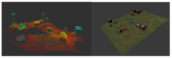
Figure 6.
First scenario point cloud and Blender model.
The algorithm waits for the vehicle to travel the minimum distance of m or the accumulated point cloud reaches its maximum size of points to start the downsampling. Each voxel of the Voxel Grid filter was defined to cm. The environment was simulated for several values of maximum sphere radius and search points in the plane detection stage. Finally, potential spots slope greater than or standard deviation along the z-axis greater than m were rejected.
Figure 7 shows a comparison of the execution time between the downsampling step and the PCA stage for several simulations with increased number of search points. The downsampling technique is relatively fast, taking about 20 ms. Moreover, increasing the number of search points implies more iterations for the PCA algorithm. Considering that the PCA is applied in a downsampled point cloud, downsampling the point cloud is justified because it limits the sample size.
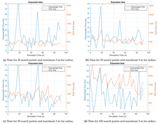
Figure 7.
Comparison between downsampling and PCA execution time for the first simulation.
Regarding the number of detected spots, it is not possible to obtain a precise analysis of the performance of the algorithm in this simulation. This is due to the fact that the environment has many regions for landing. Table 3 summarizes the results for the simulation. It also presents the simulation results with fixed search points but increasing maximum radius. The PCA run-time increases rapidly to a small increase in radius. This implies that the value chosen for the neighborhood radius has greater weight in this step.
Table 3.
Results for the simulation of the first case.
5.1.3. Environment II
A second environment (displayed in Figure 8) was developed in Blender with the intention of evaluating the performance of the algorithm in a bad scenario with few landing spots. The set consists of six rectangular surfaces that represent the desired landing spots surrounded by a mountain like structures. Considering the environment and the dimension of each surface, the simulations were realized for four different search points. In this simulation, the standard deviation was decreased to m.
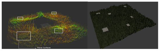
Figure 8.
Second scenario point cloud and Blender model.
Figure 9 shows a comparison of the execution time between the downsampling step and the PCA stage for several simulations with increased number of search points. For the simulations in Figure 9a,b, the run-time of the PCA algorithm was similar to the downsampling stage. The reason for this is that the planes are immediately rejected. Since the environment has a high variance in z, the angle between the normal vector calculated by the PCA and the vertical vector () is generally greater than the maximum allowed. As a result, the algorithm does not perform many iterations for the same search point.
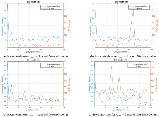
Figure 9.
Comparison between downsampling and PCA execution time for the second simulation.
Considering the detected spots, Figure 10 shows the results obtained from the simulation. The landing surfaces are the red rectangles, and the black crosses are the detected spots. However, the algorithm was not able to find a landing spot in all planes. In this scenario, one drawback of the algorithm is that if the random search point falls near a high deviation zone like the surface edges, and the algorithm may discard the plane or detect a spot outside the surface, such as a result for 100 search points (Figure 10d).
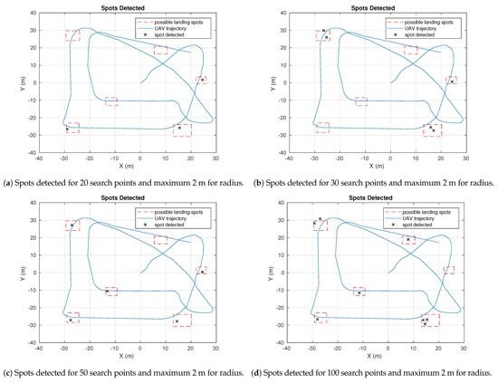
Figure 10.
Spots detected for the second scenario with different parameters.
For a better understanding of how the best landing spot varies during the simulation, Figure 11 displays the graphs of the best spot score and the score of each detected area for the case with 50 search points. Furthermore, when a spot is detected or is considered the best spot, it is marked on the graph. As the vehicle moves away from the spot, the grade associated with it decreases. If another spot has a higher score, then it becomes the new best spot.
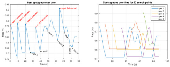
Figure 11.
Grades of the best spot and each spot detected for 50 search points.
Table 4 summarizes the results for the second simulation. The PCA mean run-time is smaller than the downsampling mean time in the first test. The difference between rejected and accepted plans increased considerably as expected.
Table 4.
Results for the simulation of the second case.
After this procedure, new simulations with different values for the voxel size were carried out to comprehend the influence of the voxel size on the other steps of the algorithm. Table 5 presents the results obtained. It was chosen as the number of search points . As the value of the voxel increases, the size of the new point cloud decreases considerably. This result shows that it is necessary to adjust the variable correctly, as it can lead to a great loss of information about the environment. Furtherore, after 1 m of voxel size, the algorithm stopped detecting landing points. In terms of the PCA performance, the increase in size did not reflect a major change in the execution time. However, the number of detected planes increased, indicating that the downsampled point cloud did not present as many obstructions as it should.
Table 5.
Results for several values of voxel size.
5.2. Experimental Dataset
5.2.1. Experimental Setup
The multirotor UAV STORK (shown in Figure 12) is an autonomous aerial vehicle with ss designed to achieve real-time data acquisition and processing efficiently. It has been used for several applications, including power lines inspection and mapping. The UAV was built, allowing a modular payload assembly, i.e., the sensor can be replaced by others that supply different types of data and using the same frame [45].
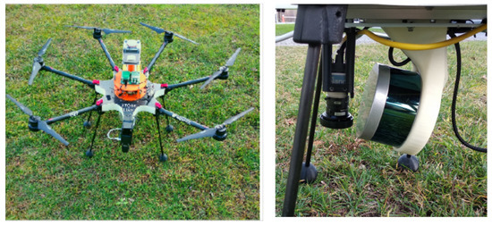
Figure 12.
STORK UAV equipped with the LiDAR VLP-16.
The UAV can operate in both manual and autonomous modes. Currently, the UAV Stork’s low-level control is accomplished by a customized autopilot (INESC TEC Autopilot), while an onboard computer ODROID-XU4 performs the high-level control. In terms of navigation, the UAV possesses two IMUs and two GNSS receivers. In addition to the low-cost sensors, STORK also has the high-performance IMU STIM300 and the single-band GNSS receiver ComNav K501G that supports Real-Time Kinematic (RTK). Generally, this setup of sensors succeeds in satisfying the requirements for many applications.
Regarding the perception assembly, the sensors to extract information about the surrounding area, the UAV STORK, has two visual cameras (Teledyne Dalsa G3-GC10-C2050 and FLIR Point- Grey CM3-U3-13S2C-CS) and a 3D spinning LiDAR sensor (Velodyne VLP-16). These sensors provide data used as input for processing algorithms in several modules, such as navigation and 3D reconstruction. For instance, the Velodyne VLP-16 data is the input for the emergency landing spot detection algorithm.
5.2.2. Dataset
The experimental dataset corresponds to the staircase of the Monastery of Tibães, Braga, Portugal. The stairway consists of several water fountains that are intertwined by stairs. This area has numerous trees that hinder the navigation and localization of the UAV and are considered obstacles for detecting landing points.
Two experiments were performed to assemble this dataset. First, the vehicle started by mapping a field of vegetation near the staircase (see Figure 13a). After that, the UAV traveled through the different levels of the stairway. The second experiment was done at the monastery building, specifically on the fence of the monastery (Figure 13b). This region consists mainly of buildings and vegetation. It is an open area with more landing spots.
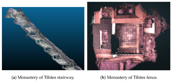
Figure 13.
3D reconstruction of the Monastery of Tibães.
In this experiment, the landing spot detection algorithm was evaluated with more restrictive parameters. Planes with standard deviation along the z-axis greater than cm were rejected. In addition, the maximum allowed radius for a spot was m, and the maximum point cloud size for starting the downsampling algorithm was 30,000 points. In addition, it was chosen as the number of search points .
5.2.3. Dataset Results
For a better understanding of the algorithm procedure, in Figure 14 and Figure 15, we identified the detected spots along with the camera image in the current timestamp of the operation. The red lines represent the center of the spot found during the plane detection step. The small red lines are detected spots that were not chosen as the best landing zones. It is worth noting that some of the detected landing spots are part of a larger spot. Besides the fact that the search points are chosen at random, another reason that justifies this behavior is the need for the maximum radius not to be too large so that the plan detection algorithm does not consume much time, as previously demonstrated by the simulations.
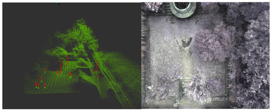
Figure 14.
Point cloud, spots, and camera image near a water fountain.
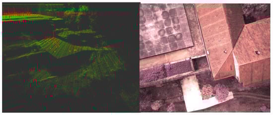
Figure 15.
Point cloud, spots, and camera image near entrance.
Moreover, the best spot grade has been stored and shown in Figure 16. The result obtained illustrates the effect of the weights in the spot classification stage. For instance, since the maximum allowed value for the standard deviation is very restrictive, relatively safe zones can be chosen as the best spot even with a low score.
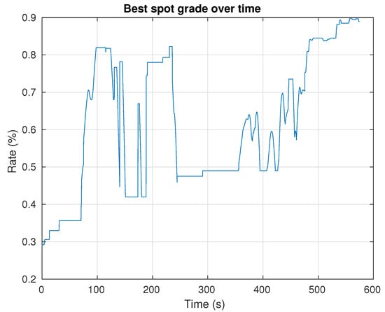
Figure 16.
Rating of the best spot for the dataset.
Table 6 presents some statistics obtained for the experiment. In order to obtain the influence of the algorithm on the computer’s energy consumption, the consumption rate was measured before initializing the algorithm and afterwards. An average increase of 2.96 W was observed. Additionally, the detected spots had an average radius of 3.24 m.
Table 6.
Statistics for the experimental dataset.
Similarly to the simulation of the second environment, the algorithm’s performance was evaluated for several sizes of voxels. Table 7 displays the results. The results obtained are similar to the simulation in relation to the loss of information with the voxel increase. However, a considerable reduction in the execution time of the plane detection step was observed. One explanation is that the dataset has more landing zones compared to the second simulated environment. Therefore, many iterations are performed in the PCA step, unlike the simulation, where there are only a few planar surfaces. In addition, the number of detected spots reduced with the increasing voxel size.
Table 7.
Results for several values of voxel size in the dataset.
6. Discussion
Some considerations concerning the acquired results have been already discussed in Section 5. The algorithm was able to detect safe landing spots in simulation and also during the experimental dataset. Downsampling the accumulated point cloud proved to be very useful. The plane detection algorithm is the most demanding in terms of processing time and memory consumption. This is expected due to the loop nature of this part of the algorithm. Therefore, in the downsampling step, reducing the number of points while maintaining a faithful representation of the environment becomes essential to decrease the execution time in the following steps.
Regarding the experimental field test, the point cloud was generated based on LiDAR data at an approximate rate of 10 Hz. Consequently, the algorithm can run in real-time as the algorithm processes the data and outputs a spot in less than 100 ms. However, this depends on the parameters chosen by the user, namely the size of the accumulated point cloud and the number of search points in the plane-detection loop. The plane detection algorithm had an average execution time of 37.87 ms. Therefore, we can see the good computational efficiency of the algorithm. In terms of physical memory, the average usage was 14.90 MB for a total of 8GB of the computer. It was also possible to conclude the algorithm’s energy only added an average of 2.96 W to the consumption rate regarding energy consumption.
One limitation of the algorithm is that it does not guarantee that a landing point will be found due to the random approach to choosing the search point from the point cloud. However, the results showed that, by gradually increasing the neighborhood sphere’s radius, the algorithm could obtain a satisfactory region to detect the planes.
7. Conclusions and Future Work
This paper addressed the development of a real-time emergency landing detection method based on LiDAR for UAVs. Methods like the one presented in this paper will allow us to have more safety during UAV out-of-sight missions. The proposed algorithm was evaluated in a simulation environment to characterize the robustness under different conditions and also in an experimental dataset during a 3D reconstruction mission in the staircase of the Monastery of Tibães, Braga, Portugal. The overall results showed the algorithm’s ability in both cases, i.e., simulation and experimental datasets, to detect the landing spot in real-time and continuously recalculate new landing spots during a UAV mission based on the parameters defined in Table 2. To the best of the authors’ knowledge, this paper contributes to the global system solution to provide emergency landing spots and the implementation of Voxel Grid Filter for point cloud compression. This step allows the algorithm to considerably decrease the number of points while maintaining an adequate representation of the environment.
As future work, we intend to validate the proposed algorithm under different surfaces with water and snow. These regions can reflect the light beams of the LiDAR, and the algorithm would consider areas with slopes equal to zero. Therefore, it would be chosen as a landing point. Furthermore, it is also interesting to benchmark the algorithm performance with other data-structuring techniques regarding computational time and spot detection. Another research work will integrate more weighting factors (wind speed, battery status, etc.) that could be considered during the spot evaluation layer.
Author Contributions
Conceptualization, G.L. and A.D.; data curation, G.L.; formal analysis, G.L.; investigation, G.L.; methodology, G.L.; project administration, A.D., A.M. and J.A.; resources, A.D.; software, G.L.; supervision, A.D., A.M. and J.A.; validation, G.L.; visualization, G.L.; writing—original draft, G.L.; writing—review and editing, G.L., A.D., A.M. and J.A. All authors have read and agreed to the published version of the manuscript.
Funding
This work is financed by National Funds through the Portuguese funding agency, FCT—Fundação para a Ciência e a Tecnologia, within project UIDB/50014/2020.
Conflicts of Interest
The authors declare no conflict of interest.
Abbreviations
The following abbreviations are used in this manuscript:
| EKF | Extended Kalman Filter |
| GNSS | Global Navigation Satellite System |
| GPS | Global Positioning System |
| IMU | Inertial Measurement Unit |
| LiDAR | Light Detection and Ranging |
| LMS | Least Mean Square |
| MORSE | Modular Open Robots Simulation Engine |
| PCA | Principal Component Analysis |
| PROSAC | Progressive Sample Consensus |
| RADAR | Radio Detection Furthermore, Ranging |
| ROS | Robot Operating System |
| RTK | Real-Time Kinematic |
| UAV | Unmanned Aerial Vehicle |
References
- Demir, K.A.; Cicibas, H.; Arica, N. Unmanned Aerial Vehicle Domain: Areas of Research. Def. Sci. J. 2015, 65, 319–329. [Google Scholar] [CrossRef]
- Liew, C.F.; DeLatte, D.; Takeishi, N.; Yairi, T. Recent developments in aerial robotics: A survey and prototypes overview. arXiv 2017, arXiv:1711.10085. [Google Scholar]
- Singhal, G.; Bansod, B.; Mathew, L. Unmanned Aerial Vehicle Classification, Applications and Challenges: A Review. Preprints 2018, 2018110601. [Google Scholar] [CrossRef]
- Sousa, P.; Ferreira, A.; Moreira, M.; Santos, T.; Martins, A.; Dias, A.; Almeida, J.; Silva, E. Isep/inesc tec aerial robotics team for search and rescue operations at the eurathlon challenge 2015. In Proceedings of the 2016 International Conference on Autonomous Robot Systems and Competitions (ICARSC), Bragança, Portugal, 4–6 May 2016; pp. 156–161. [Google Scholar]
- De Cubber, G.; Doroftei, D.; Serrano, D.; Chintamani, K.; Sabino, R.; Ourevitch, S. The EU-ICARUS project: Developing assistive robotic tools for search and rescue operations. In Proceedings of the 2013 IEEE International Symposium on Safety, Security, and Rescue Robotics (SSRR), Linköping, Sweden, 21–26 October 2013; pp. 1–4. [Google Scholar]
- Azevedo, F.; Dias, A.; Almeida, J.; Oliveira, A.; Ferreira, A.; Santos, T.; Martins, A.; Silva, E. Real-time lidar-based power lines detection for unmanned aerial vehicles. In Proceedings of the 2019 IEEE International Conference on Autonomous Robot Systems and Competitions (ICARSC), Porto, Portugal, 24–26 April 2019; pp. 1–8. [Google Scholar]
- Aghaei, M.; Grimaccia, F.; Gonano, C.A.; Leva, S. Innovative automated control system for PV fields inspection and remote control. IEEE Trans. Ind. Electron. 2015, 62, 7287–7296. [Google Scholar] [CrossRef]
- Loureiro, G.; Soares, L.; Dias, A.; Martins, A. Emergency Landing Spot Detection for Unmanned Aerial Vehicle. In Iberian Robotics Conference; Springer: Berlin/Heidelberg, Germany, 2019; pp. 122–133. [Google Scholar]
- Loureiro, G.; Dias, A.; Martins, A. Survey of Approaches for Emergency Landing Spot Detection with Unmanned Aerial Vehicles. In Proceedings of the Robots in Human Life—CLAWAR’2020 Proceedings, Moscow, Russia, 24–26 August 2020; pp. 129–136. [Google Scholar]
- Johnson, A.E.; Klumpp, A.R.; Collier, J.B.; Wolf, A.A. Lidar-based hazard avoidance for safe landing on Mars. J. Guid. Control Dyn. 2002, 25, 1091–1099. [Google Scholar] [CrossRef]
- Whalley, M.; Takahashi, M.; Tsenkov, P.; Schulein, G.; Goerzen, C. Field-testing of a helicopter UAV obstacle field navigation and landing system. In Proceedings of the 65th Annual Forum of the American Helicopter Society, Grapevine, TX, USA, 27–29 May 2009. [Google Scholar]
- Whalley, M.S.; Takahashi, M.D.; Fletcher, J.W.; Moralez, E., III; Ott, L.C.R.; Olmstead, L.M.G.; Savage, J.C.; Goerzen, C.L.; Schulein, G.J.; Burns, H.N.; et al. Autonomous Black Hawk in Flight: Obstacle Field Navigation and Landing-site Selection on the RASCAL JUH-60A. J. Field Robot. 2014, 31, 591–616. [Google Scholar] [CrossRef]
- Chamberlain, L.; Scherer, S.; Singh, S. Self-aware helicopters: Full-scale automated landing and obstacle avoidance in unmapped environments. In Proceedings of the 67th Annual Forum of the American Helicopter Society, Virginia Beach, VA, USA, 3–5 May 2011; Volume 67. [Google Scholar]
- Scherer, S.; Chamberlain, L.; Singh, S. Autonomous landing at unprepared sites by a full-scale helicopter. Robot. Auton. Syst. 2012, 60, 1545–1562. [Google Scholar] [CrossRef]
- Scherer, S.; Chamberlain, L.; Singh, S. Online assessment of landing sites. In Proceedings of the AIAA Infotech@ Aerospace 2010, Atlanta, GA, USA, 20–22 April 2010; p. 3358. [Google Scholar]
- Scherer, S. Low-Altitude Operation of Unmanned Rotorcraft. 2011. Available online: http://citeseerx.ist.psu.edu/viewdoc/download?doi=10.1.1.206.5553&rep=rep1&type=pdf (accessed on 14 May 2021).
- Preparata, F.P.; Shamos, M.I. Computational Geometry: An Introduction; Springer Science & Business Media: Berlin/Heidelberg, Germany, 2012. [Google Scholar]
- Maturana, D.; Scherer, S. 3d convolutional neural networks for landing zone detection from lidar. In Proceedings of the 2015 IEEE International Conference on Robotics and Automation (ICRA), Seattle, WA, USA, 26–30 May 2015; pp. 3471–3478. [Google Scholar]
- LeCun, Y.; Boser, B.E.; Denker, J.S.; Henderson, D.; Howard, R.E.; Hubbard, W.E.; Jackel, L.D. Handwritten digit recognition with a back-propagation network. In Advances in Neural Information Processing Systems; Morgan Kaufmann: Burlington, MA, USA, 1990; pp. 396–404. [Google Scholar]
- Lorenzo, O.G.; Martínez, J.; Vilariño, D.L.; Pena, T.F.; Cabaleiro, J.C.; Rivera, F.F. Landing sites detection using LiDAR data on manycore systems. J. Supercomput. 2017, 73, 557–575. [Google Scholar] [CrossRef]
- Yan, L.; Qi, J.; Wang, M.; Wu, C.; Xin, J. A Safe Landing Site Selection Method of UAVs Based on LiDAR Point Clouds. In Proceedings of the 2020 39th Chinese Control Conference (CCC), Shenyang, China, 27–29 July 2020; pp. 6497–6502. [Google Scholar]
- Bosch, S.; Lacroix, S.; Caballero, F. Autonomous detection of safe landing areas for an UAV from monocular images. In Proceedings of the 2006 IEEE/RSJ International Conference on Intelligent Robots and Systems, Beijing, China, 9–15 October 2006; pp. 5522–5527. [Google Scholar]
- Fitzgerald, D.; Walker, R.; Campbell, D. A vision based forced landing site selection system for an autonomous UAV. In Proceedings of the 2005 International Conference on Intelligent Sensors, Sensor Networks and Information Processing, Melbourne, VIC, Australia, 5–8 December 2005; pp. 397–402. [Google Scholar]
- Fitzgerald, D.L. Landing Site Selection for UAV Forced Landings Using Machine Vision. Ph.D. Thesis, Queensland University of Technology, Brisbane, Australia, 2007. [Google Scholar]
- Mejias, L.; Fitzgerald, D.L.; Eng, P.C.; Xi, L. Forced landing technologies for unmanned aerial vehicles: Towards safer operations. Aer. Veh. 2009, 1, 415–442. [Google Scholar]
- Warren, M.; Mejias, L.; Yang, X.; Arain, B.; Gonzalez, F.; Upcroft, B. Enabling aircraft emergency landings using active visual site detection. In Field and Service Robotics; Springer: Berlin/Heidelberg, Germany, 2015; pp. 167–181. [Google Scholar]
- Eendebak, P.; van Eekeren, A.; den Hollander, R. Landing spot selection for UAV emergency landing. In Unmanned Systems Technology XV. International Society for Optics and Photonics; SPIE Defense, Security, and Sensing: Baltimore, MD, USA, 2013; Volume 8741, p. 874105. [Google Scholar]
- Forster, C.; Faessler, M.; Fontana, F.; Werlberger, M.; Scaramuzza, D. Continuous on-board monocular-vision-based elevation mapping applied to autonomous landing of micro aerial vehicles. In Proceedings of the 2015 IEEE International Conference on Robotics and Automation (ICRA), Seattle, WA, USA, 26–30 May 2015; pp. 111–118. [Google Scholar]
- Hinzmann, T.; Stastny, T.; Cadena, C.; Siegwart, R.; Gilitschenski, I. Free LSD: Prior-free visual landing site detection for autonomous planes. IEEE Robot. Autom. Lett. 2018, 3, 2545–2552. [Google Scholar] [CrossRef]
- Kaljahi, M.A.; Shivakumara, P.; Idris, M.Y.I.; Anisi, M.H.; Lu, T.; Blumenstein, M.; Noor, N.M. An automatic zone detection system for safe landing of UAVs. Expert Syst. Appl. 2019, 122, 319–333. [Google Scholar] [CrossRef]
- Bektash, O.; Pedersen, J.N.; Gomez, A.R.; la Cour-Harbo, A. Automated Emergency Landing System for Drones: SafeEYE Project. In Proceedings of the 2020 International Conference on Unmanned Aircraft Systems (ICUAS), Athens, Greece, 1–4 September 2020; pp. 1056–1064. [Google Scholar]
- Serrano, N. A bayesian framework for landing site selection during autonomous spacecraft descent. In Proceedings of the 2006 IEEE/RSJ International Conference on Intelligent Robots and Systems, Beijing, China, 9–15 October 2006; pp. 5112–5117. [Google Scholar]
- Kyburg, H.E. Probabilistic reasoning in intelligent systems: Networks of plausible inference by Judea Pearl. J. Philos. 1991, 88, 434–437. [Google Scholar] [CrossRef]
- Howard, A.; Seraji, H. Multi-sensor terrain classification for safe spacecraft landing. IEEE Trans. Aerosp. Electron. Syst. 2004, 40, 1122–1131. [Google Scholar] [CrossRef]
- Quigley, M.; Conley, K.; Gerkey, B.; Faust, J.; Foote, T.; Leibs, J.; Wheeler, R.; Ng, A.Y. ROS: An Open-Source Robot Operating System; ICRA Workshop on Open Source Software; ICRA: Kobe, Japan, 2009; Volume 3, p. 5. [Google Scholar]
- Soares, E.; Brandão, P.; Prior, R. Analysis of Timekeeping in Experimentation. In Proceedings of the 2020 12th International Symposium on Communication Systems, Networks and Digital Signal Processing (CSNDSP), Porto, Portugal, 20–22 July 2020; pp. 1–6. [Google Scholar] [CrossRef]
- Freepik. Flat Drone. Available online: https://www.freepik.com/free-vector/basic-variety-of-flat-drones_1348538.htm (accessed on 11 October 2020).
- DNS. ODROID-XU4. Available online: https://cdn.antratek.nl/media/product/d9e/odroid-xu4-octa-core-computer-with-samsung-exynos-5422-g143452239825-47c.jpg (accessed on 11 October 2020).
- Orts-Escolano, S.; Morell, V.; García-Rodríguez, J.; Cazorla, M. Point cloud data filtering and downsampling using growing neural gas. In Proceedings of the The 2013 International Joint Conference on Neural Networks (IJCNN), Dallas, TX, USA, 4–9 August 2013; pp. 1–8. [Google Scholar]
- Meagher, D.J. Octree Encoding: A New Technique for the Representation, Manipulation and Display of Arbitrary 3-d Objects by Computer; Electrical and Systems Engineering Department Rensseiaer Polytechnic: Troy, NY, USA, 1980. [Google Scholar]
- Mosa, A.S.M.; Schön, B.; Bertolotto, M.; Laefer, D.F. Evaluating the benefits of octree-based indexing for LiDAR data. Photogramm. Eng. Remote. Sens. 2012, 78, 927–934. [Google Scholar] [CrossRef]
- Echeverria, G.; Lemaignan, S.; Degroote, A.; Lacroix, S.; Karg, M.; Koch, P.; Lesire, C.; Stinckwich, S. Simulating complex robotic scenarios with MORSE. In International Conference on Simulation, Modeling, and Programming for Autonomous Robots; Springer: Berlin/Heidelberg, Germany, 2012; pp. 197–208. [Google Scholar]
- Echeverria, G.; Lassabe, N.; Degroote, A.; Lemaignan, S. Modular open robots simulation engine: Morse. In Proceedings of the 2011 IEEE International Conference on Robotics and Automation. Citeseer, Shanghai, China, 9–13 May 2011; pp. 46–51. [Google Scholar]
- The MORSE Simulator Documentation. Available online: https://www.openrobots.org/morse/doc/stable/morse.html (accessed on 6 October 2020).
- Azevedo, F.; Dias, A.; Almeida, J.; Oliveira, A.; Ferreira, A.; Santos, T.; Martins, A.; Silva, E. Lidar-based real-time detection and modeling of power lines for unmanned aerial vehicles. Sensors 2019, 19, 1812. [Google Scholar] [CrossRef] [PubMed]


Publisher’s Note: MDPI stays neutral with regard to jurisdictional claims in published maps and institutional affiliations. |
© 2021 by the authors. Licensee MDPI, Basel, Switzerland. This article is an open access article distributed under the terms and conditions of the Creative Commons Attribution (CC BY) license (https://creativecommons.org/licenses/by/4.0/).