Abstract
Complex dielectric constant (CDC) of bound water determines the accuracy of the complex dielectric constant of wet soil. According to electrical double-layer structure and dielectric properties, the bound water on clay particle surface is divided into strongly bound water and weakly bound water. Based on this classification, models for the complex dielectric constants of bound water and soil are established taking into consideration factors such as temperature, moisture, texture, and microwave frequency. The results show that the fundamental reason why the complex dielectric constant of bound water is between that of ice and free water is the adsorption force which forms the electrical double-layer structure on the surface of clay particles. Low-concentration cationic solution could exist in free soil water and was found as the reason for the higher salinity and conductivity of free soil water, as compared to the measured soil solution. Results of soil CDC model are in good agreement with measured data across a wide range of microwave frequencies and soil temperature, moisture, and texture. The absolute root mean square error analysis also shows that the soil CDC model in this paper compared to the other models is more accurate.
1. Introduction
The physical process of soil moisture retrieval by microwave remote sensing involves two steps. The complex dielectric constant (CDC) of soil is first calculated using the radiation signal received by the sensor. Secondly, the moisture is obtained by the soil complex dielectric constant models which include the complex relationship between soil moisture and its CDC. Thus, the study of soil dielectric property via physical means is crucial for the soil moisture retrieval by microwave remote sensing [1,2,3].
The effective CDC of mixtures in nature is often expressed as a function of the CDC of inclusions and the background as well as the inclusion volume fraction [4]. Soil is a porous medium composed of air, dry soil, bound water, and free water [4,5,6]. Of the four, the CDC of air and dry soil are constant, and that of free water can be calculated by the Debye equation. The only unknown parameter is the CDC of bound water (εb). Thus, the εb and the volume content of bound water (Vb) determine the accuracy of soil CDC. Bound water, also known as adsorbed water or hygroscopic water, is mainly found on the surface of clay particles, and forms as a result of the surface effect of these particles [7,8]. The dielectric property of soil water (mainly bound water) differs from that of the water extracted from the same soil. When soil minerals are exposed to water, the exchangeable cations on the surface of clay particles enter the solution, forming cationic solution around the particles. These ions that contribute to conductivity will re-enter soil particles after water is removed [7,9]. The CDC of bound water thus cannot be measured directly. Existing methods mostly perform indirect assessment on the results of the CDC model for bound water through the measured soil CDC [5,6].
Existing soil semi-empirical complex dielectric models have explored and simulate the CDC of bound water. Wang and Schmugge [10] suggest a value for the CDC of bound water between those of free water and ice, and formulate its equation for bound water as a linear combination of the CDC of ice and free water. Dobson et al. [5] establish two mixing models for soil CDC. The first one is a four-component complex dielectric mixing model in which the complex dielectric constants of bound water are expressed by the permittivity of ice, 5‰ saline waterm and empirical estimation (35-j15), respectively. The second model is a more general semi-empirical complex dielectric model for soil in which Dobson established a modified Debye equation which can be used to calculate the CDC of total soil water (both free water and bound water). Peplinski et al. [11] perform another fitting on the empirical parameters of the general semi-empirical complex dielectric model by Dobson et al. [5] and expand the application of the model to the 0.3–1.3 GHz frequency range. Boyarskii et al. [12] make measurements on the relaxation time of bound water at the surface of clay particles and construct a dielectric model for bound water with the number of molecular layers of bound water as the independent variable. Mironov et al. [6,13,14] believe that two specific soil moisture regions exist in which alteration in the soil dielectric property is generated solely by increment in bound water or free water, while their CDC are held constant. Liu et al. [15] made improvements on the Wang–Schmugge [10] soil dielectric model by modifying CDC of bound water and free water which is based on the new Debye relaxation spectrum and in turn depends on soil texture. Although studies show bound water is the electrical double-layer solution at the surface of clay particles [5,7], current methods for calculating the complex dielectric constant of bound water lack theoretical support of soil chemistry and do not take into consideration the comprehensive effect of soil temperature, moisture, and texture, and microwave frequency.
The calculation of the CDC of soil requires the amount of bound water as an input parameter. Wang and Schmugge [10] define the concept of transition moisture to make the distinction between bound water and free water. Soil water above the transition moisture is defined as free water, and soil water below the transition moisture is bound water. In their four-component soil complex dielectric mixing model, Dobson et al. [5] treat the clay particle surface as an infinite plane, and the content of bound water is the product of the thickness of the adsorption-layer and the specific surface area. In the soil semi-empirical complex dielectric model, Dobson et al. [5] treat the dielectric property of free water and that of bound water as one entity, and do not calculate the bound water content separately. Mironov et al. [6,13,14] introduce the maximum bound water content to distinguish between bound water and free water. Park et al. [16] calculated the bound water content by using the wilting point and porosity. As the bound water content defined by Dobson et al. [5] is the adsorption-layer solution and not the entire electrical double-layer solution, and both the transition moisture and maximum bound water content are derived by fitting of measured data, existing calculations on bound water content thus still fall short in terms of the research on the properties of bound water.
In summary, to address the above issue, the following goals are set forth in this paper: (1) establishing an appropriate method for computing the content of bound water (both strongly bound water and weakly bound water); (2) developing a complex dielectric constant model for bound water based on the electrical double-layer theory; (3) establishing a simple and convenient soil complex dielectric constant model using the as-developed bound water CDC model; (4) elucidating the fundamental reason of the special properties of the CDC of bound water in terms of surface effect and adsorption force. The layout this paper is as follows: the electrical double-layer theory is explained in Section 2; the complex dielectric constant models for bound water and wet soil are established in Section 3 and Section 4, respectively; results and discussion are given in Section 5 and Section 6.
2. The Electrical Double-Layer Model: Introduction and Application
Bound water is often treated as the electrical double-layer (EDL) of solution on the clay particle surface [5,7]. Hence, the existing Stern-Gouy electrical double-layer theory is used to describe the microscopic structure at the clay particle surface and calculate the microscopic physical quantities of soil. Although the theory of EDL in soil system has been discussed in many publications [17,18,19,20,21], quantitative calculations concerning DEL are still complicated. Here a derivation of the Stern-Gouy DEL and quantitative calculations for five soils with different textures are presented.
As shown in Figure 1, the EDL consists of surface charges and anti-ion solution. As the lattice of a clay particle is incomplete, the clay particle surface is negatively charged, and the anti-ion is positive. Based on the absorption force acting on the EDL, the anti-ion solution is further divided into the adsorption-layer and diffuse-layer. Some ions are immobilized to the clay particle surface by the van der Waals force, chemical bonds, and electrostatic attraction to form an adsorption-layer (also known as the Stern-layer). The remaining ions are dispersed in the solution phase by electrostatic force, forming the diffuse-layer (also known as Gouy-layer). The concentration of cations in the diffuse-layer decreases exponentially with the distance from the adsorption layer-diffuse layer interface. All equations (Equations (1)–(6)) in this section are taken from Olphen [19,20] and Shang et al. [21].
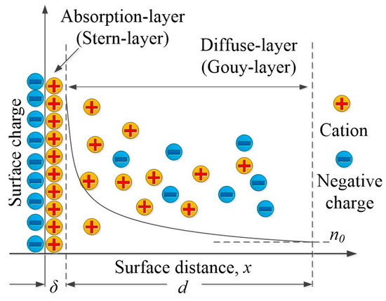
Figure 1.
Illustration of the electrical double-layer model; δ is the thickness of adsorption-layer; d is the thickness of the diffuse-layer; n0 is the soil solution concentration.
The total amount of negative charges on the clay particle surface (σ) is the sum of charges in the adsorption layer (σ1) and diffuse layer (σ2):
The amount of charges in the adsorption-layer can be approximated statistically using the number of cation adsorption sites and adsorption force, and is expressed as follows:
where n1 is the number of adsorption sites per square centimeter on mineral particle surface. Assuming that each site occupied by water molecules within a single layer is a potential cation adsorption site, the number of adsorption sites on the surface is then n1 ≈ 1015 sites/cm2. The following quantities are also defined: ν ≈ 2 is the average valence of cations in diffuse-layer of the five soil samples in Table 1; e = 1.602176634 × 10⁻¹⁹ C is the charge on a single electron; NA = 6.02 × 10²³ is the Avogadro constant; Mw = 18.01528 g/mol is the molecular weight of the solvent; n0 is the concentration of soil solution; Φδ is the electric potential of the adsorption layer; Ψ = 0 is the specific adsorption potential at clay particle surface; k = 1.38 × 10⁻²³ J/K is the Boltzmann constant; T′ is the thermodynamic temperature.

Table 1.
Soil physical parameters for calculating the electric double-layer model.
The charge (σ2) in the diffuse-layer can be expressed as function of the soil solution concentration (n0) and the Stern potential (Φδ):
where ε = 80 is the average dielectric constant of the diffuse-layer solution. When both the surface charge density (σ) and soil solution concentration (n0) are known, the Stern potential (Φδ) could be obtained. All physical parameters pertaining EDL can be calculated from the Stern potential. The thickness (d) of the diffuse-layer is expressed as follows:
The relationship between ion concentration in the diffuse-layer (n) and the distance (x) is:
where x is the distance between the diffuse layer and the adsorption layer-diffuse layer interface, and the parameters β and K are defined as , .
The average ion concentration in a sublayer of the diffuse-layer with thickness x2 − x1 is:
The parameters of electrical double-layer and measurements of soil complex dielectric constants are obtained from [5,22]. The five different soil texture surveyed are representative of the sand and clay content in typical soil types, as per the classification of the U.S. Department of Agriculture, in which sand is any soil with particle diameter of d > 0.05 mm, silt is soil with particle diameter of 0.002 mm < d < 0.05 mm, and clay is soil with particle diameter of d < 0.002 mm.
3. Bound Water Model and Model Parameters
The complex dielectric constant (CDC) of bound water is closely related to the distance from the clay particle surface. The bound water film at the clay particle surface is tightly bound to these particles. The real part of the dielectric constant is close to that of ice [5]. As the thickness of bound water film increases, the CDC of the water layer farther away from the solid surface gradually approaches that of free water [5,23]. As such, the CDC of bound water is between that of ice and free water. According to the electrical double-layer structure, the bound water is divided into strongly bound water and weakly bound water. Strongly bound water is the very thin layer of adsorption solution at the surface of clay particle. Weakly bound water refers is the diffuse-layer solution outside the regime of strongly bound water but under the influence of the electric field generated by the surface charges. As the two types of bound water differ in their content and property, the methods of their CDC are also different.
3.1. Content of Strongly Bound Water
The adsorption-layer possesses certain particular properties. Although the type of exchangeable cations, concentration of soil solution, distribution of charges, and irregular shape of clay particle surface all affect the adsorption of cations, these factors have a weak influence on the thickness of the adsorption layer. Verwey and Overbeek [24] and Olphen [19,20] show that most of the adsorption-layer charges are found within 5 Å from the clay particle surface. Shang et al. [21], however, think that the thickness of the adsorption-layer varies between 5 and 6.5 Å. Tripathy et al. [25] suggest a reasonable thickness of adsorption-layer of 5 Å. Dobson et al. [5] use 3.6 Å as the thickness of the adsorption-layer to calculate the content of bound water. Based on the above, δ=5 Å is chosen as the adsorption-layer thickness in this paper. Treating the clay particle surface as planar [5], and taking in to consideration the linear relationship between specific surface area and the content of strongly bound water [26,27], the maximum volume of strongly bound water (Vmaxsb) is:
where AS is the specific surface area and ρb is the soil bulk density. The exponent of 0.9 is included to correct for the content of strongly bound water with respect to the specific surface area.
3.2. Dielectric Constant of Strongly Bound Water
The complex dielectric constant of the adsorption-layer solution (εsb) is largely determined by the degree of binding between water molecules and clay particles and the nature of surface charges on clay particles [21]. Olphen [19,20] assigns a value of 6 to εsb. Sridharan and Satyamurty [28] and Shang et al. [21] point out that εsb could vary between 3 and 6 or 4 and 8, respectively. Wang and Schmugge [10] and Campbell [29] reach the conclusion that εsb at the mineral surface is close to that of ice (εsb = 3.5–3.8). Dobson et al. [5] assume that soil particles are covered by a thin layer of chemically bound water with a dielectric constant of εsb = 3.2 + j0.1. As the diameter of bound water molecules is 2.5 [19,20] or 2.8 Å [12], the adsorption-layer thus contains roughly two layers of bound water film. The first layer has CDC close to that of ice, but the CDC of the second layer is difficult of assess. As shown in Figure 2, the relaxation times of the first two layers of bound water molecules on the clay particle surface are 5.0 × 10⁻¹⁰ and 5.0 × 10⁻¹¹ s, respectively [12]. Assuming the CDC of the first layer of bound water equals that of ice (εi = 3.2 + j0.1), and the CDC of the first two layers of water follow the Debye equation [30], the CDC of the second layer of water is found to be 16 + j0.5 using the relaxation time of the first two layers. This value is about five times the former. The CDC of strongly bound water adopts the following equation:
where W is the soil moisture. Equation (8) necessarily implies that when soil moisture (W) is greater than the maximum content of strongly bound water (Vmaxsb), the dielectric constant of strongly bound water adopts a constant value of 9 + j0.6. When soil moisture (W) is less than the maximum content of strongly bound water (Vmaxsb), the dielectric constant of strongly bound water is determined by the ratio of soil moisture to the maximum content of strongly bound water.
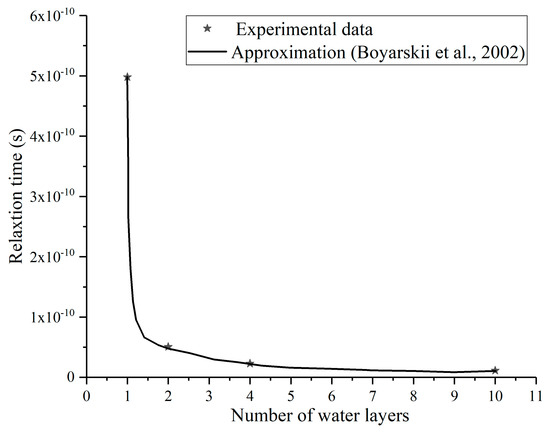
Figure 2.
Fitting of the relationship between the relaxation time of bound water and the number of bound water layers on the soil particle surface. The fitting curve and measurements of this figure come from [12].
3.3. Content of Weakly Bound Water
Taking into account the nonlinear relationship between the maximum content of bound water content (Vmaxb) and the specific surface area, the model for unfrozen water content is used here to calculate Vmaxb. At temperature below 0 °C, unfrozen water is formed between ice and the soil particle surface due to adsorption and capillary action at the soil particle surface [31]. Based on its property, unfrozen water is categorized either as capillary water or bound water. As soil cools, capillary water would freeze before bound water, and the latter only begins to freeze when capillary water is completely frozen. The maximum content of bound water is readily computed using the model of unfrozen water content when the initial freezing point of bound water (T1) is known. Referencing the transition moisture [10], maximum content of bound water [6,13,14], and the initial freezing point of bound water [32,33,34], this paper defines the Vmaxb as approximately the unfrozen water content at −2 °C. Applying the unfrozen water model of Anderson and Tice (1973), the maximum volume of bound water is:
where T1 = 2 is the absolute value of the negative temperature, and the parameters C and D (, ) are both related to the specific surface area of soil (AS). The result of the original equation for unfrozen water [35] is given in mass percentage, and needs to be converted into volume fraction of water by multiplying it with soil bulk density (ρb) and the coefficient 0.01, which results in Equation (9).
The content of weakly bound water (Vwb) is thus the difference between the maximum volume of bound water and that of strongly bound water:
3.4. Dielectric Constant of Weakly Bound Water
The complex dielectric properties of strongly bound water and weakly bound water in soil are different. Weakly bound water defined by this paper is the diffuse-layer solution. The dielectric property of unfrozen water has been experimentally proven to be similar to that of salt solutions [5,22]. Thus, the Debye equation for salt solutions is used here to calculate the dielectric constant of weakly bound water. As Figure 2 shows, the relaxation time varies slightly for water molecules in the 3rd to 10th layer on the clay particle surface (the first two layers of water molecules are the adsorption-layer solution, and the 3rd to 10th layer of bound water are the diffuse-layer solution). With the presence of such a moisture range in soil, the increment of bound water is the cause for the change in the soil dielectric constant in this moisture range [6,13,14]. For this reason, instead of the concentration of a salt solution, the average cation concentration in the 1st to 8th layer of water molecules in the diffuse-layer of five soil samples is used to calculate the CDC of weakly bound water (εwb):
where Ssw is the salinity, f is the frequency, and T is the soil temperature. The 1st to 8th layer of water molecules in the diffuse layer has a thickness of about 20 Å. The average cation concentration of the five soil samples is approximately 0.36 mol/L (Table 1), which is equivalent to a salinity of Ssw ≈ 20.9 ‰ of sodium chloride solution. Equation (11) shows the following: when , the CDC of weakly bound water is equal to that of 20.9‰ sodium chloride solution. is the Debye equation for salt solutions, and is expressed as [36]:
where εsw∞ is the dielectric constant at the high-frequency limit of salt solution, which is assumed to equal the value of 4.9. f is the wave frequency in Hz. εsw0 is the static dielectric constant of pure water, and τsw is the relaxation time of pure water in s. ε0 is the dielectric constant for free space, which is 8.854 × 10⁻¹² F/m. σi is the effective conductivity of salt solution in S/m. εsw0, τsw, and σi are all related to temperature and salt content:
3.5. Dielectric Constant of Bound Water
The electrical double-layer (EDL) model describes the microscopic structure of clay particles. As shown in Table 1, despite the differences in soil texture, the input parameters (surface charge density (σ) and soil solution concentration (n0)) and output parameters (average diffuse-layer thickness (d) and parameter β) for the EDL model of the five soil samples are not significantly different. Soil texture mainly affects the specific surface area and not the parameters related to EDL. The average values of the EDL-related parameters for the five soil samples of Table 1 are therefore representative of a wide array of fixed-charge soils. Hence, this parametric model for the complex dielectric constant of bound water (εbw) established on the EDL structure is universal. εbw is the product of the CDC of strongly bound water (εsb) and weakly bound water (εwb) with their respective volumes:
The expression of εwb changes with soil moisture. Equations (8)–(13) are known collectively as the model for the complex dielectric constant of bound water.
4. Soil Dielectric Mixing Model
Many natural substances are, strictly speaking, a mixture of different components. Their complex dielectric constants thus result from the combination of the CDC of each component [4]. The particle size, particle orientation, volume fraction, and dielectric constant of each component affect the dielectric constant of the whole mixture [4,37,38,39,40]. Researchers have developed several dielectric models for CDC of natural mixtures [41,42,43,44,45,46]. For easier computation and application, the most concise of them, the four-component dielectric mixing model [5] is used in this paper, and its equation is:
The subscripts soil, air, ss, f, and b refer to moist soil, air, dry soil, free water, and bound water, respectively. In the equation, , ρs is the specific density, and P is the porosity. . When , and ; when , and . εair = 1 + j0, εss = 4.7 + j0.2 [5]. εb is calculated by Equation (13). As free water contains a certain amount of salt [10,15], 8‰ salt solution is used here as free soil water. α is the shape factor, reflecting the geometry of soil particles [47] and is closely related to the internal structure and depolarization factor of soil [48]. α adopts different values in different dielectric mixing models. In the semi-empirical soil dielectric mixing model [5], α = 0.65; in the generalized refractive mixing dielectric model, α = 0.5; in the Looyenga mixing model [46], α = 0.333. In the mixed model of this paper, α = 0.55 for the microwave frequency range of 1.4–4 GHz, and α=0.65 for the microwave frequency range of 4–18 GHz.
Similar to the CDC of bound water (εb), the soil complex dielectric constant (εsoil) displays considerable piecewise characteristics. Equation (14) can be expressed as:
Using Equation (15), the prediction of soil complex dielectric involves the following steps:
1. The moisture (W), temperature (T), specific surface area (AS), specific density (ρS), and bulk density (ρb) of soil are measured. The volume of dry soil (VSS), porosity (P), and air volume (Vair) are then calculated from these physical quantities.
2. The maximum content of strongly bound water (Vmaxsb), maximum content of bound water (Vmaxb), and content of weakly bound water (Vwb) are found from Equations. 7, 9, and 10. The content of free water (Vf) is calculated from soil moisture (W) and the maximum content of bound water (Vmaxb).
3. The complex dielectric constants (εsb and εwb) of strongly bound water and weakly bound water are calculated using Equations (8) and (11). The complex dielectric constants (εb and εf) of bound water and free water are then calculated from Equations (12) and (13), respectively.
4. The volume fractions and complex dielectric constants of air, dry soil, bound water, and free water are substituted into the four-component soil dielectric mixing model (Equation (15)) to obtain the dielectric constant of soil.
Specific surface area (AS) is an important input parameter of soil dielectric mixing model. Considering most of the measured soil data contain particle size distribution, a recommended algorithm in predicting specific surface area based on soil particle size distribution is as follows [49]:
The soil complex dielectric mixing model developed here partitions soil water into strongly bound water, weakly bound water, and free water. This is a more precise classification than existing models [5,6,10]. In this study, the classification of bound water is based on the EDL structure at the clay particle surface. Four main assumptions are made in the calculation of the complex dielectric constant of bound water: (1) the dielectric property of the first layer of strongly bound water resembles that of ice; (2) the complex dielectric constant of the second layer of strongly bound water is about five times that of the first; (3) for Vmaxsb < V < Vmaxb, change in CDC of wet soil is caused by the increment of weakly bound water; (4) the CDC of weakly bound water is equivalent to that of salt solution.
5. Data and Results
The values of the soil complex dielectric constant used in this paper are from the measurements of five types of natural soil by [5,22]. These data consist of two parts: the first is the particle size, specific surface area, and surface charge density of these five types of soil (Table 1), and the second part is their measured soil complex dielectric constants (Figure 3) at 0–50% relative humidity and four individual microwave frequencies (1.4, 5, 10, and 18 GHz). These five types of natural soil represent a wide range of sand and clay content. The measured values of soil dielectric constant cover a broad array of soil moisture (0–50%), microwave frequencies (1.4–18 GHz), and details in soil microscopic physical quantities.
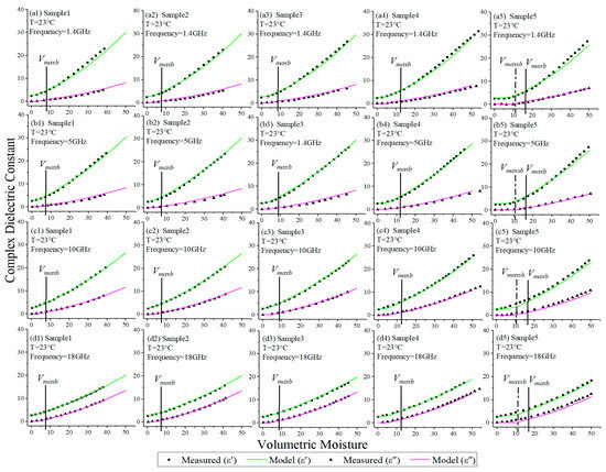
Figure 3.
Comparison between results of the soil mixing complex dielectric model (Equation (15)) and measured data for real part and imaginary part; the black vertical line represents the maximum bound water content (Vmaxb); the black vertical dotted line represents the maximum strongly bound water content (Vmaxsb). (a1–a5) represents five types of soil in Table 1 at 1.4 GHz, respectively; (b1–b5) represents five types of soil in Table 1 at 5 GHz, respectively; (c1–c5) represents five types of soil in Table 1 at 10 GHz, respectively; (d1–d5) represents five types of soil in Table 1 at 18GHz, respectively.
Figure 3 shows the results of the soil complex dielectric mixing model (Equation (15)). The dielectric constant of bound water is calculated from Equation (13). The measured complex dielectric constants of the five soil samples agree well with the model results across the four individual microwave frequencies (1.4, 5, 10, and 18 GHz) and 0–50% relative humidity. Soil moisture is the main factor influencing soil complex dielectric constant. The latter shows significant change with soil moisture, and both its real part and imaginary part are strongly dependent on soil moisture. An inspection of the green curves (the real part of soil complex dielectric constant) of Figure 3a1–a5 reveals the maximum content of bound water (Vmaxb). The slope of curve above this value behaves differently from that below this value. Above this value, the slope is almost invariant as moisture increases. Below this point, it increases gradually with moisture. This indicates the change in soil dielectric constant and the increase in of free water at W ≥ Vmaxb. Using the slope of the green curve in Figure 3a5, the soil dielectric constant can be partitioned into three segments: 0 < W < Vmaxsb (Stage I); Vmaxsb ≤ W < Vmaxb (Stage II); W ≥ Vmaxb (Stage III). At frequencies of 1.4 and 5 GHz (Figure 3a1–a5,b1–b5), the slope of soil complex dielectric constant (real part and imaginary part) of Stage III is significantly higher than that of Stage I or Stage II. At high moisture levels (Stage III), the increase in soil complex dielectric constant is due to free water increments, while at lower moisture levels (Stages I and II), this increase is due to bound water increments. The above result means the dielectric constant of free water is higher than that of bound. At W < Vmaxb (Stage I), the curve is almost flat, which means at this stage, the dielectric constant of bound water is almost equal to that of dry soil. The slope of Stage II (Vmaxsb ≤ W < Vmaxb) is greater than that of Stage I but less than that of Stage III. This means that strongly bound water possesses very different dielectric property compared to weakly bound water. At W < Vmaxb, the slope of the green curve increases gradually, indicating gradual rise in the dielectric constant of bound water with soil moisture. The dielectric constant of bound water at the proximity of clay particle surface resembles that of ice, while at farther distance, it approaches that of free water. Based on the above analysis and double layer structure, we define the bound water of Stage I as strongly bound water. At this stage, change in soil complex dielectric constant is caused by the increment of strongly bound water. The bound water of Stage II is a combination of strongly bound water with some weakly bound water, and change in the soil complex dielectric constant is caused by the increment of weakly bound water. The soil water of Stage III includes both bound water and free water, and change in the soil dielectric constant is caused by the increment of free water.
As shown in Figure 3, curves for the real part and imaginary part of the soil dielectric constant have almost the same intercept at W=0 across the various individual microwave frequencies. This means the dielectric constants of dry soil and air hardly change with microwave frequency. In Figure 3a5,b5,c5,d5, the soil complex dielectric constant displays substantial dispersion across the frequencies. Its real part decreases while the imaginary part increases as the frequency increases. Soil texture also affects the complex dielectric constant of soil. For soil samples 1, 3, and 5, the maximum content of strongly bound water and the maximum content of bound water (Table 2) both increase with soil specific surface area, indicating a higher level of bound water in soil with more clay content. The maximum content of strongly bound water has an approximately linear relation with soil specific surface area, while a nonlinear relationship exists between maximum bound water content and soil specific surface area. For each individual microwave frequency, the real part and the imaginary part of the dielectric constant of soil sample 5 (soil sample with the highest clay content) are smaller than other soil samples. This is mainly because of the higher level of bound water in a soil sample with more clay and the smaller real part of bound water dielectric constant than free water. For this reason, when soil moisture is the same, the soil sample with more clay would have a higher level of bound water and less free water, and a smaller soil dielectric constant (real part and imaginary part).
Table 2.
Parameters and part results of complex dielectric constant model of bound water.
The salt content of free water needs to be considered when modeling the soil dielectric constant. Wang and Schmugge [10] and Liu et al. [15] both believe that the salt content of free soil water is higher than that of the salt concentration of real soil solution and it increases with the content of clay. This can be explained using the electrical double-layer model. In Figure 4, the cation concentration in the vicinity of the clay particle surface decreases exponentially with the distance to the surface. The transition moisture and maximum bound water content given by soil dielectric models [6,10,15] do not take into account the entire cationic solution and leave out the portions of low-concentration cationic solution dispersed in free water. As cationic solution only exists at the surface of clay particles, higher clay content would mean a greater proportion of cationic solution in free water, and higher salinity of the entire soil solution.
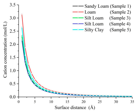
Figure 4.
Variation of cation concentration in diffuse-layer with distance from adsorption layer-diffuse layer interface; the curves were drawn based on the calculation results from the Equation (5); physical properties of soils are shown in Table 1.
For the imaginary part of the soil complex dielectric constant at low frequency range, Liu et al. [15] suggest the introduction of an effective conductivity loss term related to soil water. The reason might be related to the unique properties of the imaginary part of the salt solution dielectric constant. In Figure 5, near 1.4 GHz frequency, the imaginary part of the salt solution dielectric constant is significantly higher than that of pure water, while in the 4–20 GHz range, little difference is seen between the imaginary parts of the two dielectric constants. The conclusion is that at the 1.4 GHz frequency, salt makes the prediction of the imaginary part more difficult for the dielectric constant of free water. As such, Liu et al. [15] adjust the conductivity term to negate the influence of cationic solution in free water.
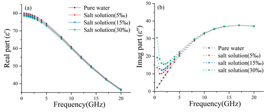
Figure 5.
Complex dielectric constant of (a) real part and (b) image part of pure water and salt solutions; the models of pure water and salt solution are from [30] and [36], respectively.
6. Discussion
6.1. Change of Bound Water Dielectric Constant with Soil Moisture
Figure 6 more explicitly shows changes in the real part and imaginary part of the complex dielectric constant of bound water (εb) with soil moisture in the three stages. In Stage I (0 < W < Vmaxsb), the real part of the complex dielectric constant of strongly bound water shows linear change, and the imaginary part is almost 0. The slope of the curve becomes smaller with clay content increases. For all four frequencies, the real part of εb of sandy loam (Sample 1) shows significantly larger slope than that of silty clay (Sample 5). In Stage II (Vmaxsb ≤ W < Vmaxb), the change in εb follows a curve, and the increase in εb is produced by weakly bound water. The effect of soil texture is obvious, with smaller εb occurring at higher amounts of clay content. Stage III (W ≥ Vmaxb) has the maximum content of bound water, and the εb is independent of soil moisture but is still affected by soil texture and temperature, and microwave frequency. The influence of microwave frequency on the εb is largely manifested at Stages II and III, and is different on the real part and imaginary part. In soil samples of the same textural class, the imaginary part of the bound water dielectric constant decreases as frequency increases, while the imaginary part decreases first and then increases.
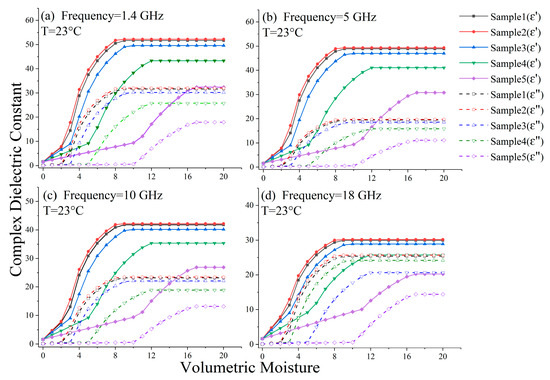
Figure 6.
The moisture dependence of the dielectric constant for bound water of five types of soil at frequencies of (a) 1.4 GHz, (b) 5 GHz, (c) 10 GHz, and (d) 18 GHz; the indicated moisture range for each soil extends between 0% and 20%; the first turning point of each curve is the maximum strongly bound water content (Vmaxsb), and the second turning point is the maximum bound water content (Vmaxb); the curves were drawn based on the results from the Equation (13); physical properties of soils are shown in Table 1.
The complex dielectric constant of the bound water falls between those of ice and free water, primarily as a result of surface effect and the adsorption force it produces. The surface effect and adsorption force can be explained by the theory of electrical double-layer. The surface effect is the combined action generated by the molecules and negative charges on the surface of clay particles. Adsorption force is the comprehensive force generated by surface effect that makes strongly bound water and weakly bound water forming special properties. On the surface of clay particles, Van der Waals force and valence force are formed by clay molecules, and electrostatic force is produced by negative charges. The adsorption force acting on the strongly bound water which is close to the surface of clay particle is the combined force of van der Waals force, valence force, and electrostatic force. The joint action of these forces stabilizes the dielectric property of strongly bound water. The adsorption force acting on the weakly bound water which is located in the outer layer of the strongly bound water is the electrostatic force, and this electrostatic force decreases exponentially with surface distance. The exponential decay of electrostatic force makes the complex dielectric constant of weakly bound water increase gradually and approach that of free water.
6.2. Change of Bound Water Dielectric Constant with Soil Temperature
Figure 7 shows the change of the complex dielectric constant of bound water (εb) with temperature at the three frequencies. Frequency dictates the change trend of εb with temperature. At 1.4 GHz, for all three soil samples, the real part of εb decreases as temperature increases, while the imaginary part increases with temperature. In contrast, at 10 GHz, the real part and the imaginary part of εb change shows the opposite change with temperature increases. The real part increases with temperature, while the imaginary part decreases. At 18 GHz, the imaginary part of εb first increases with temperature and then decreases.
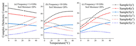
Figure 7.
The temperature dependence of the complex dielectric constant for bound water of three types of soil at frequencies of (a) 1.4 GHz, (b) 10 GHz, and (c) 18 GHz; the curves were drawn based on the results from the Equation (13); physical properties of soils are shown in Table 1.
At a fixed frequency, soil texture has a slight impact on the change of the bound water dielectric constant with temperature, and significantly affects the value of the complex dielectric constant of bound water. In Figure 7, soil samples 1, 4, and 5 have 13.43%, 19.00%, and 47.38% of clay by mass, respectively. The real part and imaginary part of the bound water dielectric constant of sample 5 (with high clay content) are significantly lower than those of samples 1 and 4 (with lower clay content). As temperature changes, sample 5 also displays slightly smaller change in the real and imaginary part of its bound water dielectric constant than samples 1 and 4. The effect of temperature on soil dielectric constant occurs via a competitive mechanism [50]. Although this conclusion is based on the real part of soil dielectric constant in the Time Domain Reflection (TDR) frequency band (about 1.4 GHz), the same competitive mechanism is followed at other frequency bands. For example, at 10 GHz, at higher temperature, the thermal motion of molecules becomes more intense, bound water content decreases, and free water content increases. However, temperature elevation also leads to increase in the dielectric constants of bound water and free water. As a result, temperature rise only increases the real part of soil complex dielectric constant.
6.3. Comparison of Soil Dielectric Mixing Models
The CDC prediction with high average accuracy is very important for estimating soil moisture by microwave remote sensing, so several soil dielectric mixed models are compared in three frequency bands (Figure 8). In the range of 0–50% relative humidity, the predicted results of soil dielectric mixing models have the same trend with the measured data, so the correlation coefficient between the results of each model and the measured data is very high. Considering that correlation coefficient has difficulty distinguishing the advantages and disadvantages of the model, we introduced the concept of absolute root mean square error (ARMSE) (Table 3) to analyze the advantages and disadvantages of soil dielectric mixed model. ARMSE is the ratio of root mean square error from the modeling results and the measurements against the measurements.
where, n represents the measured number of soil moisture in the range of 0–50%.
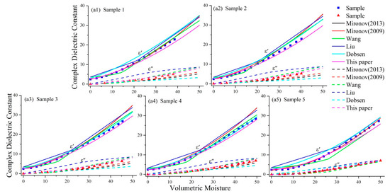
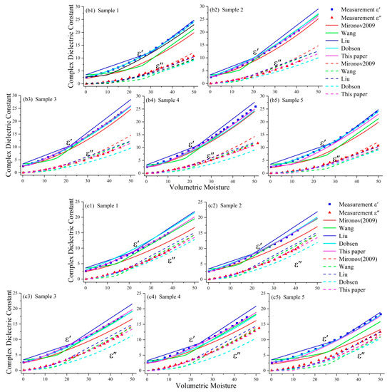
Figure 8.
Comparison of the results of different complex dielectric constant models in the moisture range of 0-50% at (a1–a5) 1.4 GHz, (b1–b5) 10 GHz and (c1–c5) 18 GHz. Model of Mironov2013 [14] is a single frequency model at 1.4 GHz. Models of Mironov2009, Wang, Liu, and Dobson are from [5,10,13,15], respectively. In the model of Wang, we used 8% salt solution instead of free water.
Table 3.
ARMSEs of experimental values and calculated values. The bold of Soil No. 1–5 represents five types of in Table 1.
According to the average ARMSEs of all models in three frequency bands, the average ARMSEs of the models in 1.4 GHz band are higher than 5 and 18 GHz, and the average ARMSEs of imaginary parts are obviously higher than that of real parts. This shows that the prediction difficulty of the 1.4 GHz band is higher than the other bands, and the prediction difficulty of imaginary part is higher than that of the real part. Considering that the dielectric properties of bound water are like salt solution, we analyzed the reasons of ARMSEs in different frequency bands according to the CDC of salt water and pure water (Figure 5). The real parts of the CDC of pure water and salt water are about 80 at 1.4 GHz, and it gradually decreases to 35 with the increase of frequency to 18 GHz. The real part of CDC of bound water lies between ice and free water, so it is more difficult to predict bound water in 1.4 GHz band than in other bands. This may be the reason why the ARMSEs of the real parts of 1.4 GHz band are higher than that of 5 and 18GHz. At 1.4 GHz band, the imaginary part of the CDC of salt solution is obviously affected by the concentration. The difference of imaginary parts between pure water and salt solution can reach tens (Figure 5). Therefore, the imaginary part of the CDC of bound water and content of bound water will significantly affect the imaginary part of soil dielectric constant, which is the reason why the average ARMSEs of the imaginary part in 1.4 GHz band are the largest and the prediction is the most difficult.
At 10 and 18 GHz bands, the average ARMSEs of the real parts of the models is around 0.1. For sample 5, Dobson model has the smallest ARMSEs (0.019, 0.027). For the other four soils, the ARMSE values of model of this paper are better than those of other models. The Liu model has the smallest ARMSEs (0.019, 0.027) of the imaginary parts of 10 and 18 GHz for sample 5. The reason is that Liu recalculated the conductivity of free water. For other four soils with low clay content, the ARMSE values of Liu model are large. The ARMSEs of sample 2 are 0.264 and 0.242 at 10 and 18 GHz, respectively. In the real part of 1.4 GHz, the ARMSE of each model has good accuracy. However, in the imaginary part of 1.4 GHz band, the ARMSE values of all the models except this paper are very large. In addition, the ARMSEs of Mironov2013 model, Liu model, and Dobson model are obviously different for soils with different clay contents (such as samples 1, 2, and 5 and samples 3 and 4). This phenomenon indicates that the effect of soil texture on the imaginary part of soil dielectric constant still needs to be improved. The influence of soil texture on prediction accuracy is obvious. At 18 GHz, the average ARMSE of the real part of sample 5 with the highest clay content is higher than that of the other four soils. The difference of the real part between bound water and free water at 18 GHz is the smallest, and the bound water content increases with the clay content, so this phenomenon shows that the bound water content calculated by each model is still not accurate enough. In summary, the soil complex dielectric constant model in this paper has good prediction results in all bands, especially in the imaginary part of 1.4 GHz which is used for soil moisture retrieval by microwave remote sensing [51]. As the imaginary part of the soil complex dielectric constant is a necessary parameter for calculating soil absorption coefficient, soil penetration depth, and air-soil interface reflectivity [6,30,51,52], the model in this paper can improve the accuracy of remote sensing inversion.
In order to get better results, some internal parameters of models do not conform to the actual situation. For example, in the Mironov2009 model, the real part of the dielectric constant of free water in 1.4 GHz band is 100, but it is actually 80. In the Liu model, the conductivity of free water in soil with low clay content is negative. These phenomena are inconsistent with the actual situation. Therefore, although the results of the mixed model of soil dielectric constant are good, it is necessary to deeply study each parameter. The ARMSEs of our model have a minimum value in almost every frequency range. These ARMSE values are stable and do not fluctuate greatly with soil texture and frequency. It shows that this model has strong adaptability.
7. Conclusions
Bound water is classified into strongly bound water and weakly bound water using the electrical double-layer (EDL) model for the clay particle surface, corresponding, respectively, to the adsorption-layer and the diffuse-layer solution. Applying this classification scheme, two models for the complex dielectric constant (CDC) of bound water and wet soil are established with microwave frequency and soil moisture, temperature, and texture as the independent variables. The models accurately describe the dielectric property of soil at the frequency range of 1.4–18 GHz and 0–50% moisture level.
The EDL structure is a representation of the microscopic structure of clay particles. The five soil samples studied have different textures but share similar physical properties of the EDL, such as surface charge density, soil solution concentration, average diffuse-layer thickness. Soil texture mainly affects the specific surface area of soil. Hence, it is reasonable to use averaged parameters of the five soil types in the construction of CDC for bound water.
The free water in the soil complex dielectric constant model has a higher content of salt than the actual soil solution. This is because free water contains a certain proportion of low-concentration cationic solution. As cationic solution is only found at the clay particle surface, higher clay content means a greater proportion of cationic solution in free water, thus higher salinity.
The complex dielectric constant of bound water falls between those of ice and free water, as a result of surface effect and adsorption force. The surface effect is the combined action generated by the molecules and negative charges on the surface of clay particles. Surface effect can produce the adsorption force. Clay molecules at the clay particle surface produce van der Waals and valence force, and the surface negative charges generate electrostatic force. The strongly bound water at close proximity to the clay surface corresponds to the adsorption-layer solution, and is predominantly under the action of the van der Waals force, valence force, and electrostatic force. Strongly bound water shows a stable dielectric property. Weakly bound water is the diffuse-layer solution and is mainly under the effect of electrostatic force. As electrostatic force decreases exponentially moving away from particle surface, the complex dielectric constant of weakly bound water increases gradually with the distance to the particle surface, eventually approaching that of free water. The nature and value of the adsorption force change with surface distance. When surface distance is less than thickness of adsorption layer, the adsorption force is essentially the resultant force of van der Waals force, chemical force and electrostatic force. When the surface distance is greater than thickness of adsorption layer and less than thickness of electrical double-layer which is the sum of the thickness of adsorption-layer and diffuse-layer, the essence of the adsorption force is electrostatic force.
Absolute root mean square error (ARMSE) is used to compare and analyze the results of existing soil CDC models. According to the average ARMSEs of all models in the three frequency band, the average ARMSEs of the models in 1.4GHz band are higher than 5 and 18 GHz, and the average ARMSEs in the imaginary part are obviously higher than that in the real part. The influence of soil texture on ARMSEs is obvious. At most frequency bands, the average ARMSE of the real part of sample 5 with the highest clay content is higher than that of the other four soils. The ARMSEs of our model have a minimum value in almost every frequency range and the ARMSE values do not fluctuate greatly with soil texture and frequency. It shows that model of this paper has strong adaptability.
The complex dielectric constant model of bound water established in this paper has limitations. This model is applicable only to fixed-charge soils possessing the similarity electrical double-layer structure. There are also shortcomings in the simulation of bound water, as the dielectric constant of real bound water changes as a smooth curve with soil moisture rather than as linear line segments. Therefore, more research should be performed on the dielectric property of bound water.
Author Contributions
Conceptualization, X.J. and W.Y.; methodology, X.J. software, X.J; validation, X.J.; formal analysis, X.J.; investigation, X.J.; resources, X.J.; data curation, X.J.; writing—original draft preparation, X.J.; writing—review and editing, X.J.; visualization, X.J.; supervision, X.J.; project administration, W.Y.; funding acquisition, W.Y., X.G. and Z.L. All authors have read and agreed to the published version of the manuscript.
Funding
This research was funded by the National Science Foundation of China (No. 41475018, 41675017) and National Key R & D Program by China (No. 2018YFB1502800).
Acknowledgments
We thank all the researchers who put forward suggestions in the process of writing and drawing. We thank Dobson et al. (1985) and Hallikainen et al. (1985) that provide the experimental data of this paper.
Conflicts of Interest
The authors declare no conflict of interest.
References
- Fung, A.K. Microwave Scattering and Emission Models and Their Applications; Artech House: Norwood, MA, USA, 1994. [Google Scholar]
- Jackson, T.J., III. Measuring surface soil moisture using passive microwave remote sensing. Hydrol. Process. 1993, 7, 139–152. [Google Scholar] [CrossRef]
- Wigneron, J.-P.; Waldteufel, P.; Chanzy, A.; Calvet, J.-C.; Kerr, Y. Two-Dimensional Microwave Interferometer Retrieval Capabilities over Land Surfaces (SMOS Mission). Remote Sens. Environ. 2000, 73, 270–282. [Google Scholar] [CrossRef]
- Jones, S.B.; Friedman, S.P. Particle shape effects on the effective permittivity of anisotropic or isotropic media consisting of aligned or randomly oriented ellipsoidal particles. Water Resour. Res. 2000, 36, 2821–2833. [Google Scholar] [CrossRef]
- Dobson, M.C.; Ulaby, F.T.; Hallikainen, M.T.; El-Rayes, M.A. Microwave Dielectric Behavior of Wet Soil-Part II: Dielectric Mixing Models. IEEE Trans. Geosci. Remote Sens. 1985, 23, 35–46. [Google Scholar] [CrossRef]
- Mironov, V.L.; Dobson, M.C.; Kaupp, V.H.; Komarov, S.A.; Kleshchenko, V.N. Generalized refractive mixing dielectric model for moist soils. IEEE Trans. Geosci. Remote Sens. 2004, 42, 773–785. [Google Scholar] [CrossRef]
- Saarenketo, T. Electrical properties of water in clay and silty soils. J. Appl. Geophys. 1998, 40, 73–88. [Google Scholar] [CrossRef]
- Ishizaki, T.; Maruyama, M.; Furukawa, Y.; Dash, J.G. Premelting of ice in porous silica glass. J. Cryst. Growth 1996, 163, 455–460. [Google Scholar] [CrossRef]
- Keller, C.V.; Frischknecht, F.C. Electrical Methods in Geophysical Prospecting; Pergamon Press: Oxford, UK, 1966; pp. 519–521. [Google Scholar]
- Wang, J.R.; Schmugge, T.J. An Empirical-Model for the Complex Dielectric Permittivity of Soils as a Function of Water-Content. IEEE Trans. Geosci. Remote Sens. 1980, 18, 288–295. [Google Scholar] [CrossRef]
- Peplinski, N.R.; Ulaby, F.T.; Dobson, M.C. Dielectric properties of soils in the 0.3-1.3-GHz range. IEEE Trans. Geosci. Remote Sens. 1995, 33, 803–807. [Google Scholar] [CrossRef]
- Boyarskii, D.A.; Tikhonov, V.V.; Komarova, N.Y. Model of Dielectric Constant of Bound Water in Soil for Applications of Microwave Remote Sensing. Prog. Electromagn. Res. 2002, 35, 251–269. [Google Scholar] [CrossRef]
- Mironov, V.L.; Fomin, S.V. Temperature and Mineralogy Dependable Model for Microwave Dielectric Spectra of Moist Soils. PIERS Online 2009, 5, 411–415. [Google Scholar] [CrossRef]
- Mironov, V.; Kerr, Y.; Wigneron, J.-P.; Kosolapova, L.; Demontoux, F. Temperature- and Texture-Dependent Dielectric Model for Moist Soils at 1.4 GHz. IEEE Geosci. Remote Sens. Lett. 2012, 10, 419–423. [Google Scholar] [CrossRef]
- Liu, J.; Liu, Q.; Li, H.; Du, Y.; Cao, B. An Improved Microwave Semiempirical Model for the Dielectric Behavior of Moist Soils. IEEE Trans. Geosci. Remote Sens. 2018, 56, 6630–6644. [Google Scholar] [CrossRef]
- Park, C.-H.; Behrendt, A.; LeDrew, E.; Wulfmeyer, V. New Approach for Calculating the Effective Dielectric Constant of the Moist Soil for Microwaves. Remote Sens. 2017, 9, 732. [Google Scholar] [CrossRef]
- Babcock, K.L. Theory of the chemical properties of soil colloidal systems at equilibrium. Hilgardia 1963, 34, 417–542. [Google Scholar] [CrossRef]
- Newman, A.C.D. Chemistry of Clays and Clay Minerals; Longman Sciences and Technology; Cambridge University Press: London, UK, 1987. [Google Scholar]
- Van Olphen, H. An Introduction to Clay Colloid Chemistry. Soil Sci. 1964, 97, 290. [Google Scholar] [CrossRef]
- Van Olphen, H.; Hsu, P.H. An Introduction to Clay Colloid Chemistry. Soil Sci. 1978, 126, 59. [Google Scholar] [CrossRef]
- Shang, J.; Lo, K.; Quigley, R. Quantitative determination of potential distribution in Stern–Gouy double-layer model. Can. Geotech. J. 1994, 31, 624–636. [Google Scholar] [CrossRef]
- Hallikainen, M.T.; Ulaby, F.T.; Dobson, M.C.; El-Rayes, M.A.; Wu, L.-K. Microwave Dielectric Behavior of Wet Soil-Part 1: Empirical Models and Experimental Observations. IEEE Trans. Geosci. Remote Sens. 1985, GE-23, 25–34. [Google Scholar] [CrossRef]
- Adamson, A.W. Physical Chemistry of Surfaces, 3rd ed.; Wiley-Interscience: Hoboken, NJ, USA, 1976; pp. 698–704. [Google Scholar]
- Verwey, E.J.W.; Overbeek, J.T.G. Theory of the stability of lyophobic colloids. J. Colloid Sci. 1955, 10, 224–225. [Google Scholar] [CrossRef]
- Tripathy, S.; Sridharan, A.; Schanz, T. Swelling pressures of compacted bentonites from diffuse double layer theory. Can. Geotech. J. 2004, 41, 437–450. [Google Scholar] [CrossRef]
- Smith, C.W.; Hadas, A.; Dan, J.; Koyumdjisky, H. Shrinkage and Atterberg limits in relation to other properties of principal soil types in Israel. Geoderma 1985, 35, 47–65. [Google Scholar] [CrossRef]
- Yukselen-Aksoy, Y.; Kaya, A. Method dependency of relationships between specific surface area and soil physicochemical properties. Appl. Clay Sci. 2010, 50, 182–190. [Google Scholar] [CrossRef]
- Sridharan, A.; Satyamurty, P.V. Potential-Distance Relationships of Clay-Water Systems Considering the Stern Theory. Clays Clay Miner. 1996, 44, 479–484. [Google Scholar] [CrossRef]
- Campbell, J.E. Dielectric Properties and Influence of Conductivity in Soils at One to Fifty Megahertz. Soil Sci. Soc. Am. J. 1990, 54, 332–341. [Google Scholar] [CrossRef]
- Ulaby, F.T.; Moore, R.K.; Fung, A.K. Microwave Remote Sensing: Active and Passive, Volume 3—From Theory to Applications; Artech House Inc.: Norwood, MA, USA, 1986. [Google Scholar]
- Dash, J.G. Thermomolecular Pressure in Surface Melting: Motivation for Frost Heave. Science 1989, 246, 1591–1593. [Google Scholar] [CrossRef]
- Jaeger, F.; Bowe, S.; Van As, H.; Schaumann, G.E. Evaluation of1H NMR relaxometry for the assessment of pore-size distribution in soil samples. Eur. J. Soil Sci. 2009, 60, 1052–1064. [Google Scholar] [CrossRef]
- Razumova, L.A. Basic principles governing the organization of soil moisture observations. Int. Assoc. Hydrol. Sci. Publ. 1965, 68, 491–501. [Google Scholar]
- Tian, H.; Wei, C. A NMR-based testing and analysis of adsorbed water content. Sci. Sin. Technol. 2014, 44, 295–305. [Google Scholar] [CrossRef]
- Anderson, D.M.; Tice, A.R. The unfrozen interfacial phase in frozen soil water systems. In Physical Aspects of Soil Water and Salts in Ecosystems; Springer: Berlin/Heidelberg, Germany, 1973; pp. 107–124. [Google Scholar]
- Stogryn, A. Equations for Calculating the Dielectric Constant of Saline Water (Correspondence). IEEE Trans. Microw. Theory Tech. 1971, 19, 733–736. [Google Scholar] [CrossRef]
- Mendelson, K.S.; Cohen, M.H. The effect of grain anisotropy on the electrical properties of sedimentary rocks. Geophysics 1982, 47, 257–263. [Google Scholar] [CrossRef]
- Kenyon, W.E. Texture effects on megahertz dielectric properties of calcite rock samples. J. Appl. Phys. 1984, 55, 3153. [Google Scholar] [CrossRef]
- Sen, P.N. Relation of certain geometrical features to the dielectric anomaly of rocks. Geophysics 1981, 46, 1714–1720. [Google Scholar] [CrossRef]
- Tyč, S.; Schwartz, L.M.; Sen, P.N.; Wong, P.Z. Geometrical models for the high-frequency dielectric properties of brine saturated sandstones. J. Appl. Phys. 1988, 64, 2575–2582. [Google Scholar] [CrossRef]
- Birchak, J.R.; Gardner, C.G.; Hipp, J.E.; Victor, J.M. High dielectric constant microwave probes for sensing soil moisture. Proc. IEEE 1974, 62, 93–98. [Google Scholar] [CrossRef]
- Bruggeman, D. Calculation of various physics constants in heterogenous substances I Dielectricity constants and conductivity of mixed bodies from isotropic substance. Annalen der Physik 1935, 24, 636–664. [Google Scholar] [CrossRef]
- Friedman, S.P. A saturation degree-dependent composite spheres model for describing the effective dielectric constant of unsaturated porous media. Water Resour. Res. 1998, 34, 2949–2961. [Google Scholar] [CrossRef]
- He, H.L.; Dyck, M. Application of Multiphase Dielectric Mixing Models for Understanding the Effective Dielectric Permittivity of Frozen Soils. Vadose Zone J. 2013, 12. [Google Scholar] [CrossRef]
- Garnett, J.C.M.; Larmor, J. Colours in metal glasses and in metallic films. Proc. R. Soc. Lond. 1904, 73, 443–445. [Google Scholar] [CrossRef]
- Sihvola, A. Electromagnetic Mixing Formulas and Applications; Institution of Engineering and Technology (IET): London, UK, 1999. [Google Scholar]
- Roth, K.; Schulin, R.; Flühler, H.; Attinger, W. Calibration of time domain reflectometry for water content measurement using a composite dielectric approach. Water Resour. Res. 1990, 26, 2267–2273. [Google Scholar] [CrossRef]
- Zakri, T.; Laurent, J.P.; Vauclin, M. Theoretical evidence for ’Lichtenecker’s mixture formulae’ based on the effective medium theory. J. Phys. D Appl. Phys. 1998, 31, 1589–1594. [Google Scholar] [CrossRef]
- Ersahin, S.; Gunal, H.; Kutlu, T.; Yetgin, B.; Coban, S. Estimating specific surface area and cation exchange capacity in soils using fractal dimension of particle-size distribution. Geoderma 2006, 136, 588–597. [Google Scholar] [CrossRef]
- Or, D.; Wraith, J.M. Temperature effects on soil bulk dielectric permittivity measured by time domain reflectometry: A physical model. Water Resour. Res. 1999, 35, 371–383. [Google Scholar] [CrossRef]
- Ebtehaj, A.M.; Bras, R.L. A physically constrained inversion for high-resolution passive microwave retrieval of soil moisture and vegetation water content in L-band. Remote Sens. Environ. 2019, 233, 111346. [Google Scholar] [CrossRef]
- Ulaby, F.T.; Moore, R.K.; Fung, A.K. Microwave Remote Sensing: Active and Passive. Volume 1—Microwave Remote Sensing Fundamentals and Radiometry; Addison-Wesley: Boston, MA, USA, 1981. [Google Scholar]


Publisher’s Note: MDPI stays neutral with regard to jurisdictional claims in published maps and institutional affiliations. |
© 2020 by the authors. Licensee MDPI, Basel, Switzerland. This article is an open access article distributed under the terms and conditions of the Creative Commons Attribution (CC BY) license (http://creativecommons.org/licenses/by/4.0/).