Article

Systematic Orbital Geometry-Dependent Variations in Satellite Solar-Induced Fluorescence (SIF) Retrievals

1
National Aeronautics and Space Administration (NASA) Goddard Space Flight Center (GSFC), Greenbelt, MD 20771, USA
2
Science Systems and Applications, Inc. (SSAI), Lanham, MD 20706, USA
3
Division of Geological and Planetary Sciences, California Institute of Technology, Pasadena, CA 91109, USA
4
Joint Center for Earth Systems Technology, University of Maryland Baltimore County, Baltimore, MD 21250, USA
5
Jet Propulsion Laboratory, California Institute of Technology, 4800 Oak Grove Drive, Pasadena, CA 91109, USA
6
Faculty of Geo-Information Science and Earth Observation (ITC), University of Twente, P.O. Box 6, 7500 AE Enschede, The Netherlands
7
Centro de Tecnologías Físicas, Universitat Politècnica de València, València, Camí de Vera s/n, 46022 València, Spain
8
Unit of Soil and Crop Sciences, School of Integrated Plant Sciences, Cornell University, Ithaca, NY 14853, USA
*
Author to whom correspondence should be addressed.
Remote Sens. 2020, 12(15), 2346; https://doi.org/10.3390/rs12152346
Submission received: 1 June 2020 / Revised: 5 July 2020 / Accepted: 13 July 2020 / Published: 22 July 2020

Abstract

:
While solar-induced fluorescence (SIF) shows promise as a remotely-sensed measurement directly related to photosynthesis, interpretation and validation of satellite-based SIF retrievals remains a challenge. SIF is influenced by the fraction of absorbed photosynthetically-active radiation at the canopy level that depends upon illumination geometry as well as the escape of SIF through the canopy that depends upon the viewing geometry. Several approaches to estimate the effects of sun-sensor geometry on satellite-based SIF have been proposed, and some have been implemented, most relying upon satellite reflectance measurements and/or other ancillary data sets. These approaches, designed to ultimately estimate intrinsic or physiological components of SIF related to photosynthesis, have not generally been applied globally to satellite measurements. Here, we examine in detail how SIF and related reflectance-based indices from wide swath polar orbiting satellites in low Earth orbit vary systematically due to the host satellite orbital characteristics. We compare SIF and reflectance-based parameters from the Global Ozone Mapping Experiment 2 (GOME-2) on the MetOp-B platform and from the TROPOspheric Monitoring Instrument (TROPOMI) on the Sentinel 5 Precursor satellite with a focus on high northern latitudes in summer where observations at similar geometries and local times occur. We show that GOME-2 and TROPOMI SIF observations agree nearly to within estimated uncertainties when they are compared at similar observing geometries. We show that the cross-track dependence of SIF normalized by PAR and related reflectance-based indices are highly correlated for dense canopies, but diverge substantially as the vegetation within a field-of-view becomes more sparse. This has implications for approaches that utilize reflectance measurements to help account for SIF geometrical dependences in satellite measurements. To further help interpret the GOME-2 and TROPOMI SIF observations, we simulated cross-track dependences of PAR normalized SIF and reflectance-based indices with the one dimensional Soil-Canopy Observation Photosynthesis and Energy fluxes (SCOPE) canopy radiative transfer model at sun–satellite geometries that occur across the wide swaths of these instruments and examine the geometrical dependencies of the various components (e.g., fraction of absorbed PAR, SIF yield, and escape of SIF from the canopy) of the observed SIF signal. The simulations show that most of the cross-track variations in SIF result from the escape of SIF through the scattering canopy and not the illumination.

Graphical Abstract

1. Introduction

Solar-induced fluorescence (SIF) is produced by the photosynthetic machinery of terrestrial vegetation and is emitted across a range of wavelengths spanning red to far-red (near-infrared, NIR) wavelengths. It has been measured with a number of aircraft- and ground-based instruments (e.g., [1,2] and references therein). SIF has also been mapped globally with several different satellite sensors over a range of spatial and temporal resolutions (see [2] for a review). Canopy-level SIF in the far-red spectral region, where most current satellite-based SIF observations are reported (wavelengths > ∼735 nm), displays a highly linear relationship with respect to gross primary production (GPP), the amount of carbon dioxide taken up by vegetation during photosynthesis, at weekly or longer time-scales (e.g., [3,4,5,6,7,8,9,10]); this result is also supported by modeling studies [11,12]. Therefore, satellite-based SIF data sets are of interest for carbon cycle and terrestrial ecosystem research and have been used in a number of studies (e.g., [7,13,14,15,16,17]). In contrast to traditional broad-band reflectance measurements, SIF has shown an excellent sensitivity to highly productive regions such as the US corn belt [3] and to vegetation in regions affected by snow cover [18,19,20,21].
SIF can be expressed in a congruent form of the light-use efficiency model [22,23] as
SIF ( λ em , SZA , VZA , RAA ) = e ( λ em , SZA , VZA , RAA ) Φ F ( SZA , λ em ) fPAR chl ( SZA ) PAR F ( SZA ) ,
where λ em is the SIF emission wavelength (peak emission at 740 nm for far-red spectral emission feature), e is the fractional amount of leaf-level emitted fluorescence that escapes the canopy at λ em in the direction of the observer, Φ F is the fluorescence yield, fPAR chl is the fraction of photosynthetically-active radiation for fluorescence (PAR F ) absorbed by chlorophyll, SZA is the solar zenith angle, VZA is the view zenith angle, and RAA is the relative azimuth angle between the sun and satellite. Another angle of interest is the phase angle, γ , the angle at a given point between the sun and satellite:
γ = cos 1 [ cos ( SZA ) cos ( VZA ) + sin ( SZA ) sin ( VZA ) cos ( RAA ) ] .
The minimum amount of shadowing occurs at zero phase angle, also known as the hot spot. Equation (1) is sometimes further simplified by combining e and Φ F into a single canopy-level yield quantity for a given sun-sensor geometry. fPAR chl and e are determined by canopy structure and leaf biochemistry, while physiological effects, including responses to various types of stress, are embedded in Φ F (e.g., [24]). Yang et al. [25] defined the product of fPAR and e as Γ rt that they termed the radiative transfer factor.
Both modeling results and observations suggest that the magnitude and variation of far-red canopy SIF are largely driven by the amount of absorbed photosynthetically-active radiation for SIF (APAR F = fPAR chl × PAR F ) (e.g., [10,26,27,28,29,30]). An ongoing challenge for SIF interpretation is disentangling the information about both vegetation structure and biochemistry expressed in spectral optical properties, from the physiological signal in Φ F that distinguishes SIF from traditional reflectance measurements (e.g., [26,28,31,32]). For example, Wittenberghe et al. [33] stressed the importance of quantifying canopy structural parameters such as leaf area index and angular distribution with reflectance data for detailed analysis of remotely-sensed SIF. In addition, it is important to account for solar-satellite geometry that impacts illumination and e in the direction of the observer (e.g., [17,25,30,34,35,36,37,38,39,40,41,42,43,44,45,46]). Vertical and horizontal inhomogeneity of vegetation canopies also affect canopy-level SIF including its angular distribution [47,48,49].
At present, data producers typically provide an adjustment factor to compute daily-average SIF from a single time of day measurement with the assumption that Φ F , fPAR chl , and e are constant throughout the day [50]. Daily-averaged SIF from different satellite instruments has been directly compared (e.g., [51]). While this accounts for differences in the top-of-atmosphere incoming irradiance, it does not account for structurally-dependent aspects of the illumination and their dependence on the ratio of direct to diffuse radiation. It also does not account for the fact that only a fraction of the total emitted SIF will be observed in a given direction at the top of canopy and that this fraction depends upon the observation geometry relative to the illumination.
Several approaches have been proposed and/or implemented to more fully account for sun–satellite geometrical dependencies of satellite SIF measurements (e.g., [25,30,37,38,39,42,43,44,45,52]). These methods rely on various ancillary data including reflectances along with theoretical and/or machine learning constructs (see e.g., [25] for a review). They have been tested using simulated measurements and observations, showing promise for dealing with angular variations in global satellite SIF data sets. Various limitations of these methods, such as for sparsely vegetated scenes where there is a substantial contribution from soil reflectance, have also been discussed (e.g., [25,44,46] and references therein).
Here, we examine the sun-sensor geometry dependence of far-red SIF, near infrared (NIR) reflectance, and two reflectance-based indices that have been proposed as proxies for Γ rt with large swath satellite sensors: the Global Ozone Monitoring Experiment 2 (GOME-2) and the TROPOspheric Monitoring Instrument (TROPOMI). We consider the range of local solar times (and thus solar zenith angles) observed systematically across the large swaths of GOME-2 and TROPOMI. Although the host satellites of GOME-2 and TROPOMI have equator crossing times that differ by hours, their orbital attributes allow SIF retrievals from these sensors to be directly compared at the same local overpass times at high latitudes in the northern hemisphere during summer, sometimes with similar viewing geometry. Using a one dimensional (1D) canopy radiative transfer model, we examine the geometry dependences of SIF, its basic components in Equation (1), as well as NIR reflectance and related indices including systematic satellite cross-track variations.

2. Data and Methods

2.1. SIF Satellite Data Sets

2.1.1. GOME-2 SIF

There are now three GOME-2 instruments flying on the operational European Meteorological Satellites (EUMETSAT MetOp) series satellites [53]. Here we used data from the MetOp-B GOME-2 (GOME-2B), launched in 2012, that operates in the nominal wide swath mode concurrently with TROPOMI. GOME-2B uses a scanning mirror to measure across its swath that has a width of 1920 km. An individual pixel in its forward scan across the swath is 40 km × 80 km at nadir and the backward scans are approximately three times larger. GOME-2 has four spectral bands ranges. Band 4 measures solar radiance and Earthshine radiance in the 593–790 nm range with 1024 spectral elements and a full-width at half maximum (FWHM) bandpass per spectral element of 0.48 nm. This band was used to retrieve SIF.
SIF was retrieved with GOME-2 using variants of a principal component analysis (PCA) technique [54,55,56]. Similar PCA approaches have been used in SIF retrievals with other satellite and ground-based instruments (e.g., [35,57,58]). Here, we used the GOME-2B SIF from the version 27 (v27) GOME-2 NASA dataset [54,59] produced with updates as noted below applied to the base unadjusted retrievals provided in that data set. This version uses a spectral fitting window covering 734–758 nm that has relatively weak water vapor absorption. Along with SIF, reflectances are provided at 670 and 780 nm. We used only the highest quality GOME-2B retrievals that passed all quality control checks described in Joiner et al. [59]. GOME-2B data are limited to solar zenith angle (SZA), < 75 and local solar times earlier than 13:00.
One change from v27 is that a new bias adjustment scheme is implemented with a machine learning neural network (NN) approach to remove documented biases [55]. These biases are thought to primarily result from temperature variations that occur in the instrument along its orbit that may lead to changes in the instrument response function or other effects that that mimic the spectral response of SIF. This is applied to the uncorrected data from the v27 data set. Five inputs to the regression approach of Joiner et al. [59] are used for the NN; the inputs are cosines of the view zenith angle (VZA), SZA, and relative azimuth angle (RAA) as well as latitude, and reflectance at 780 nm. The single output is the bias, defined as the retrieved far-red SIF over ocean for all pixels, both clear-sky and cloudy, with the assumption that SIF for the ocean pixels should be zero (an assumption justified by satellite measurements). This bias is then subtracted from the terrestrial SIF retrievals. The basic NN structure is a three layer feed forward network that was found by trial and error to produce reproduce the basic features of the bias. The two hidden layers in the NN architecture each contain eight nodes or two times the number of inputs. Additional details of the NN structure are given in Appendix A.
Training was done separately for each day of GOME-2B observations to estimate the bias adjustment. There were of the order of 600,000 samples available for training on a typical day. Previous versions of the regression bias adjustment scheme showed small discontinuities at latitudes boundaries where the scheme was applied; these were removed with the NN approach. The monthly mean bias adjustment for June 2018 (see Figure A1) shows a significant north to south gradient of more than 0.5 mW m 2 nm 1 sr 1 as well as a dependence on surface reflectance. This latitudinal dependence is thought to result from temperature changes in the instrument along its orbit that may affect the instrument response function. Note that many of the predictors of the bias adjustment (reflectance and the sun–satellite angles) overlap with those that we will relate to SIF measurements below. This bias adjustment was thus critical for proper interpretation of the GOME-2B data that follows. Because the bias adjustment uses data over ocean, where SIF was expected to be zero, it was completely independent of SIF emissions over vegetated land.
An effective cloud fraction, f c , was estimated by inverting
I meas = I clr ( 1 f c ) + I cld f c ,
where I meas , I clr , and I cld were the measured, clear-sky, and cloudy sky radiances at a particular wavelength (here we use 680 nm). Within the context of the mixed Lambertian-equivalent reflectivity (MLER) model and the independent pixel approximation (IPA), clouds were considered as opaque with a reflectivity of 0.8 (e.g., [60]), and f c is an effective rather than a geometrical cloud fraction. The MLER concept was shown to reproduce the correct amount of absorption or Rayleigh scattering for pixels with either optically thin and/or broken clouds and has been used in numerous trace-gas and cloud algorithms (e.g., [61,62]). At our wavelengths of interest, aerosols are not highly absorbing and scatter light similar to cloud particles. As such, they were treated like clouds within the MLER framework.
The calculation of f c has also been updated from v27. In v27, a climatology was used for I clr , and the f c calculation did not include atmospheric scattering or surface bidirectional effects. In this work, we used the collocated MODIS MCD43D reflectance parameters [63,64,65] to account for both of these. Specifically, we trained an NN to predict I clr at 680 nm. The NN has the same basic architecture as that applied to the bias adjustment (see Appendix A) but with a different number of inputs and hidden-layer nodes. The six inputs are the three bidirectional reflectance distribution function (BRDF) parameters for MODIS band 1 (620–670 nm) as well as the cosines of the SZA, VZA, and RAA. The number of nodes in each of the hidden layers was twelve or two times the number of inputs. The training used ten days (June 20-30, 2018, 43605 GOME-2 samples) of global collocated MCD43D and GOME-2B data. Only GOME-2B pixels with 670 nm reflectance < 0.6 were considered for training and of those reflectance data, only the 10% with the closest agreement to the band 1 reflectances were used. This was found to provide a sufficient amount of data for training. I meas from the v27 data set was used to compute f c . We use a strict filter of f c < 0.1 in our analysis involving SIF and reflectance data from GOME-2.

2.1.2. TROPOMI SIF

TROPOMI was launched on the European Space Agency (ESA) Sentinel-5 precursor (S5P) satellite in October 2017. TROPOMI measures solar irradiance and Earthshine radiance across a 2600 km swath with 448 spatial elements [66]. SIF is retrieved from TROPOMI pixels (3.5 km × 7 km at nadir) using a subset of the NIR band 6 that covers wavelengths 725–755 nm in 497 spectral elements with a FWHM of 0.38 nm. The TROPOMI SIF retrieval is similar to that of GOME-2 v27 in that it uses a PCA approach. The fitting window for the TROPOMI SIF retrieval is 743–758 nm [67]; this simplifies the retrieval as this wavelength range was nearly free of absorption by atmospheric molecules and thus absorption of the SIF signal does not need to be accurately accounted for. Quality control was applied as in Köhler et al. [67].
The TROPOMI retrievals currently include cloud information derived from collocated Visible Infrared Imaging Radiometer Suite (VIIRS) data on the Suomi National Polar–orbiting Partnership (NPP) flying in tandem with the S5P satellite. A cloud fraction for a TROPOMI pixel was defined by weighting the cloud fractions of all the VIIRS pixels contained within the TROPOMI pixel as described in Köhler et al. [67]. Therefore, the TROPOMI cloud fraction was not the same as f c computed above for GOME-2B. R NIR is not explicitly provided in the TROPOMI data set, but reflectance across the SIF retrieval fitting window can be computed using the absolute and relative SIF values provided in the data set as R 740 nm =SIF/(relative SIF)× (100 × π )/(cos(SZA) × F ), where F is the solar irradiance at 740 nm and relative SIF is defined as SIF relative to its reflectance background, defined as a percent.

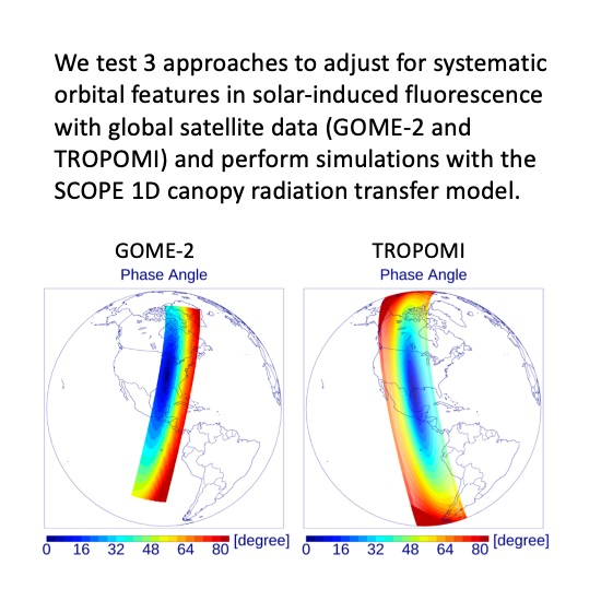
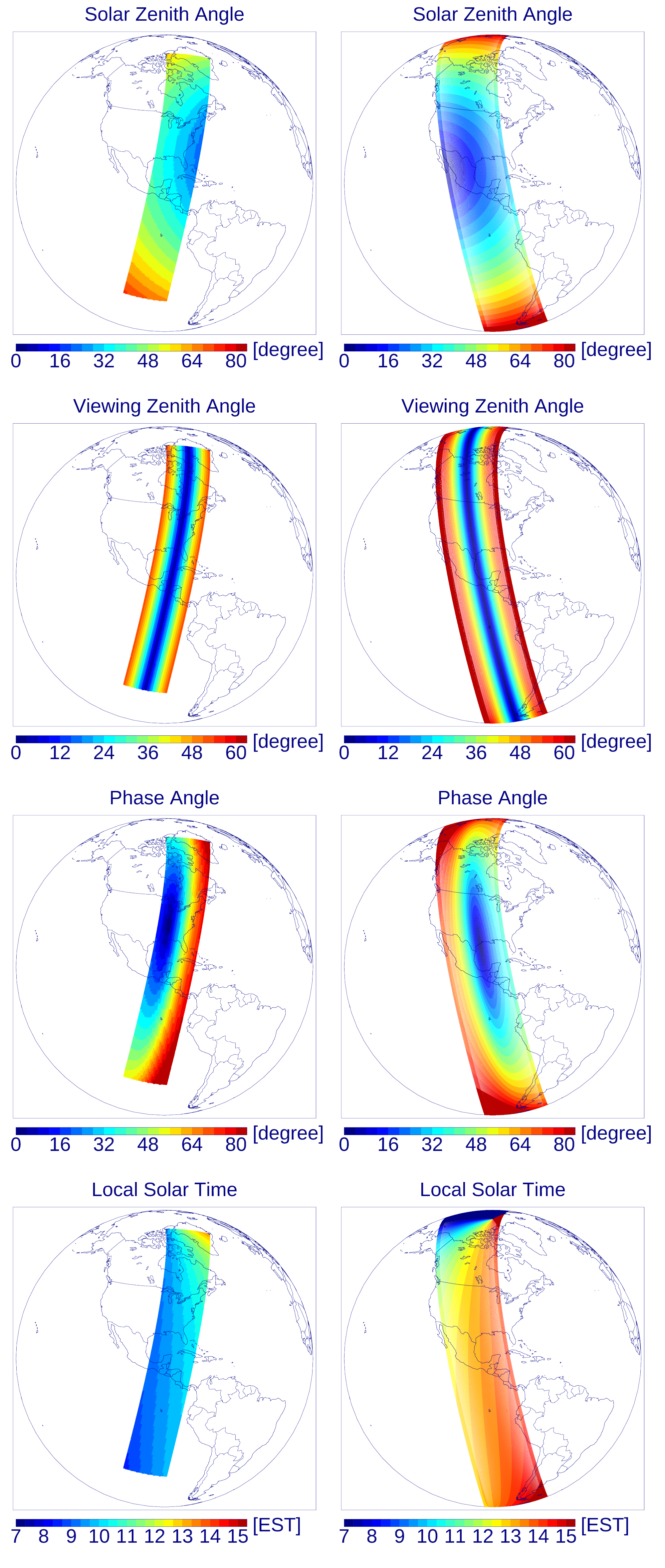
2.2. GOME-2B and TROPOMI Instrumental and Orbital Characteristics

Table 1 summarizes the main observing characteristics of the two SIF-capable instruments considered here. Both the instruments and retrievals differ in several respects. Below, we provide to our knowledge the most detailed comparison of these two data sets to date by accounting for differences in their orbital geometries.
Figure 1 shows SZA, VZA, the phase angle, and local solar times (LST) of the GOME-2B and TROPOMI observations over single orbits on 28 June 2018. The inclination angles (near 98.7 ) and nodes of the host satellites impact the local overpass times along their orbits. With GOME-2B in a descending orbit (daylight on descending node), LSTs are generally later than the 09:30 equator crossing time in the northern hemisphere (NH); for TROPOMI in its ascending node, LSTs are generally earlier than its 13:30 equator crossing time in the NH. The reverse situation occurs in the southern hemisphere.
The LSTs corresponding to individual ground footprints vary across the wide swaths of these instruments. This leads to an interesting scenario for SIF measurements; in the NH boreal summer, particularly at middle to high latitudes, there is coverage spanning a wide range of LSTs throughout the morning and early afternoon with the two instruments albeit with systematically varying sun-sensor geometries. There are measurements at the same local time with the two instruments at high latitudes in the NH, sometimes with similar viewing geometries and other times not.

2.3. Data Analysis Approach

We calculated the zonal means of the native GOME-2 or TROPOMI SIF retrievals and related parameters for 10 latitude, ten minute bins, for different plant functional types (PFTs). We did this for the month of June 2018 around the peak of the northern hemisphere growing season. To compute the zonal averages, we first averaged the data monthly into 0.5 latitude × 0.5 longitude grid boxes then aggregated the gridded data into the appropriate latitude, time, and PFT bins. Only data with cloud fractions <0.1 were used. We repeated our analysis using all data with cloud fractions <0.3 and did not find qualitatively different results although correlations between SIF/PAR and reflectances were somewhat lower on average. At the highest high northern latitudes examined here in summer months (60–70 ), GOME-2B and TROPOMI provided nearly continuous temporal coverage from 09:00 to 13:00. We computed the percentages of PFTs in each of our 0.5 gridboxes using 2017 land cover types on the climate modeling grid (CMG, 0.05 grid) derived from MODIS observations (MCD12C1 product) [68]. Only gridboxes that have a majority PFT with coverage >50% were used in our analyses.
The two approaches proposed to serve as proxies for Γ rt that we evaluate are (1) the far-red fluorescence correction vegetation index (FCVI) defined as the difference between the NIR directional reflectance ( R NIR ) and the broadband visible (VIS) directional reflectance ( R vis ¯ ) proposed by Yang et al. [25], and (2) the NIR V , defined as the product of R NIR and the normalized difference vegetation index (NDVI = ( R NIR R red )/( R NIR + R red )), i.e., NIR V = NDVI × R NIR , as proposed by Zeng et al. [44]. As the GOME-2 SIF data set includes R NIR and R red , we were able to readily compute NIR V collocated with SIF. We computed the DVI (DVI = R NIR R red ) as a proxy for FCVI.

2.4. Simulations with a 1D Canopy Radiative Transfer Model

To help interpret the satellite SIF observations, in particular the sun–satellite geometry dependences, we examined the results of SIF and reflectance simulations, including R NIR , NIR V , and DVI, from the Soil-Canopy Observation Photosynthesis and Energy fluxes (SCOPE) model version 1.70 [34]. SCOPE simulates the full radiative transfer of fluorescence from the photosystem to the top of canopy as well as reflected sunlight through the canopy. We provide a list of SCOPE input parameters for two different scenarios used in our simulations in Appendix B: (1) a C4 corn (maize) setup with a 2 m canopy height; and (2) a C3 30 m canopy designed to mimic a deeper forested type canopy. These are referred to as the C4 and C3 setups. We ran simulations for two values of leaf area index (LAI) for each setup. For the C4 case, we performed simulations for LAI = 3 and 1, and for the C3 case, we used LAI = 5 and LAI = 1. Most other parameters were similar for the two scenarios.
We note that SCOPE is a 1D model, meaning that it models vegetation as homogeneous, i.e., LAI is distributed evenly throughout the pixel with no clumping. Therefore, it does not fully capture the complexity of radiative transfer for complex and varied canopies that exists within large satellite footprints. Nevertheless, SCOPE is a useful tool for modeling general sun–satellite geometrical dependences of both SIF, as well as its individual components from Equation (1), and reflectance for a given canopy structure. It can therefore be used for a qualitative comparison with satellite measurements.
Note that the top-of-canopy irradiance in our SCOPE runs was specified as a single value regardless of the output at different solar zenith angles. That input irradiance value corresponds to a single atmospheric realization (determined by an external atmospheric radiative transfer calculation using the MODTRAN code) at an SZA of 45 . To adjust the incoming irradiance to appropriate conditions at other SZAs, the SCOPE SIF outputs were multiplied by a factor of cos(SZA)/cos(45 ). With further SCOPE simulations (1) adjusting the input irradiance to the actual magnitude of solar irradiance to fully account for the effects of irradiance on Φ F and (2) using separate external radiative transfer calculations at the appropriate SZA, we determined that the simple irradiance magnitude adjustment to SCOPE outputs was appropriate (see Appendix B for details).

3. Results

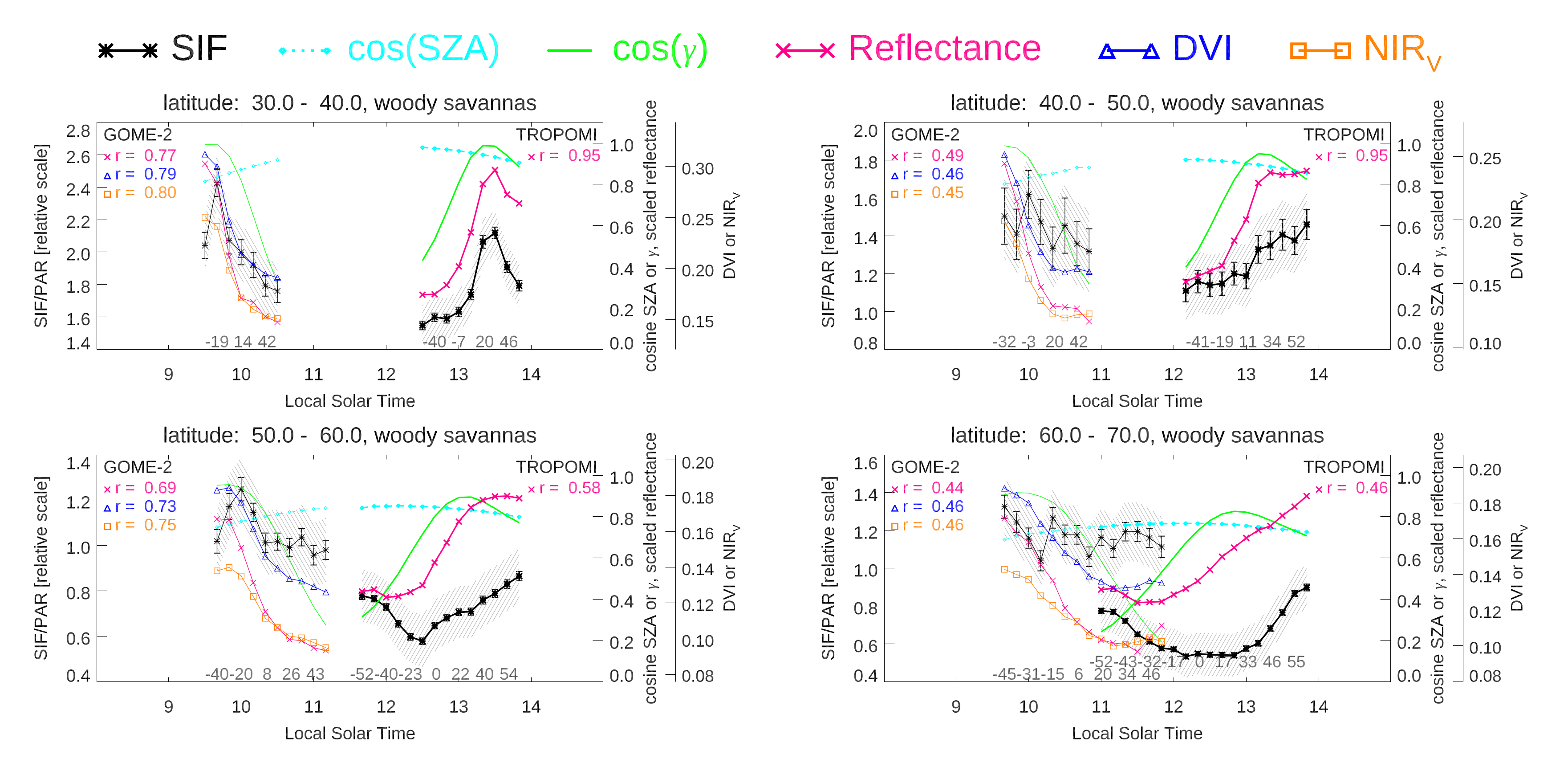
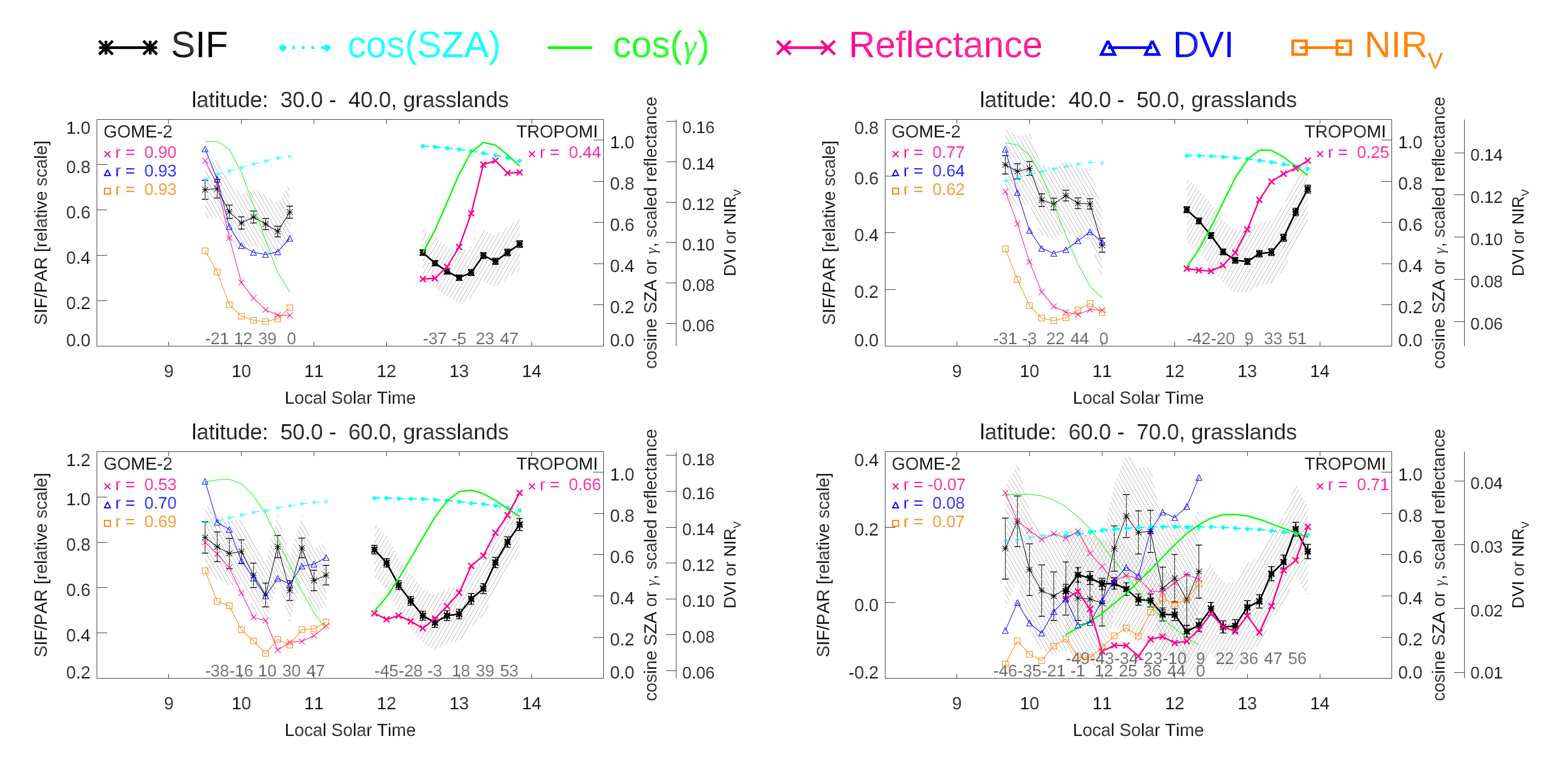
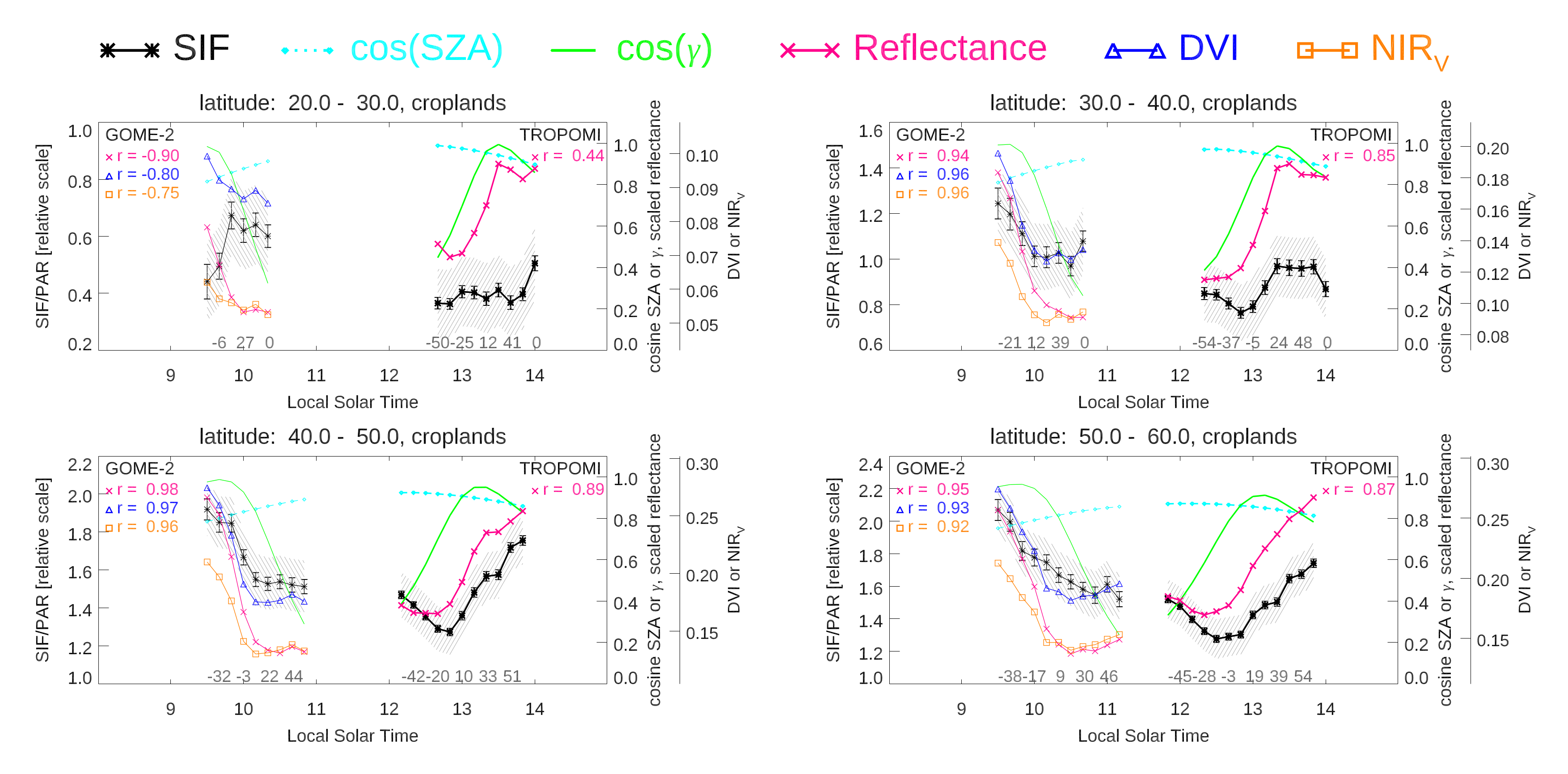
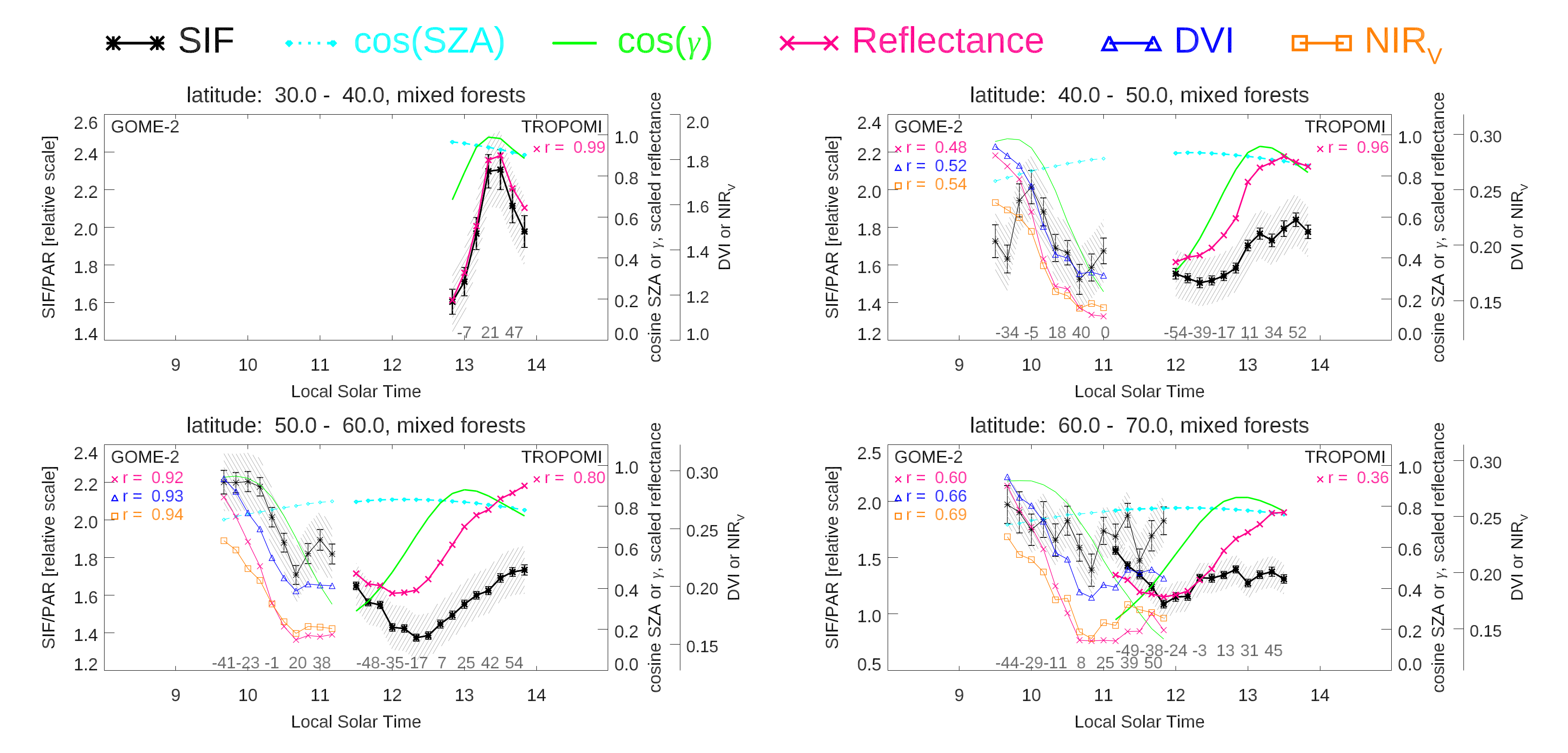
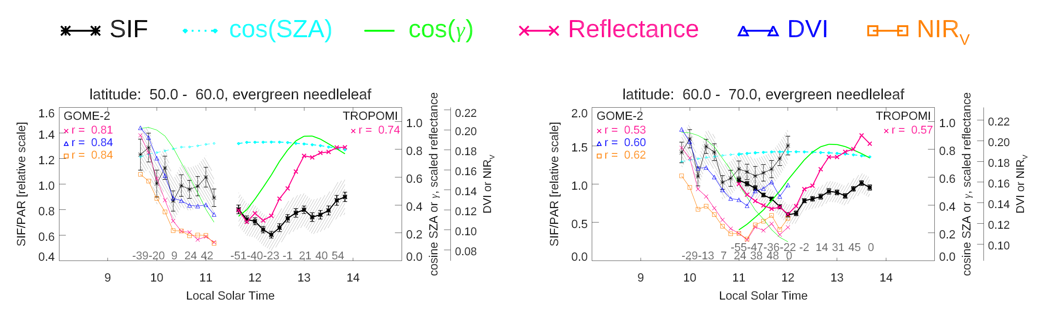
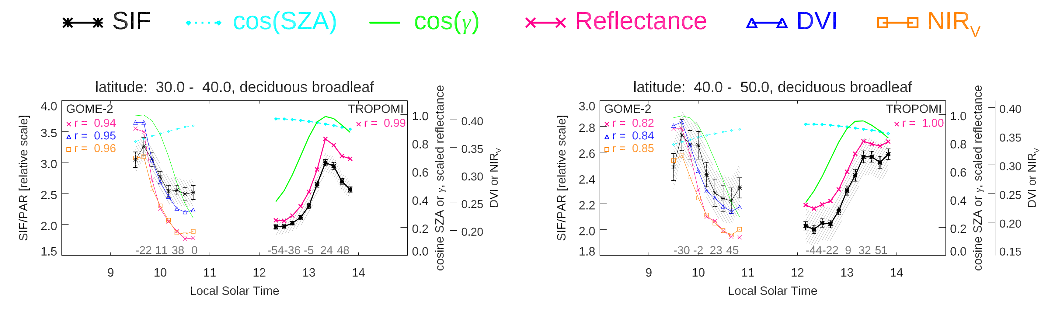
3.1. GOME-2 and TROPOMI Satellite-Based SIF and Reflectance Dependence on Illumination and View Geometry

Figure 2, Figure 3, Figure 4, Figure 5, Figure 6 and Figure 7 show SIF normalized by incoming PAR (plotted as SIF/cos(SZA) and denoted as SIF/PAR), R NIR , and satellite and solar angle information as a function of LST (or alternatively VZA) for late morning through early afternoon averaged over gridboxes dominated by different plant functional types for different latitude bins in June 2018. DVI and NIR V are shown only for GOME-2 as R red was not available in the TROPOMI SIF data set. The standard error of the mean, i.e., standard deviation of all gridbox values ( σ ) divided by N for each binned zonal average is shown by the vertical error bar and represents an uncertainty due to random errors. A conservative empirical estimate of the systematic error (0.1 mW/m 2 /nm/sr for SIF/PAR) is shown with the shading. Correlations between the binned SIF/PAR averages and the corresponding R NIR and available reflectance-based indices are also provided, separately for GOME-2 and TROPOMI. Correlations will similarly be computed using SCOPE 1D simulations below and then may be compared with those from satellite observations. Individual satellite SIF observations are dominated by retrieval noise and this makes it difficult to interpret results at the pixel level; this is why we have conducted our analysis on zonal averages. The correlations are computed for the binned averages and contain only a limited number of points per PFT and latitude range. We note that even though we average hundreds of individual pixels per bin, one or two noisy or questionable binned data points may substantially degrade the correlations.
Particularly at the higher northern latitudes, the top-of-atmosphere solar irradiance, that is proportional to cos(SZA) and indicated in the figures, does not change dramatically over the hours shown (varies by ∼20% from 09:00–13:30). The systematic variation in VZA as a function of LST is also apparent owing to the fact that LST varies across the satellite swath. The cos( γ ) variation across the swath is also shown with the highest values for GOME-2 (lowest amount of shadowing) on the western part of its swath and the highest values on eastern swath portion for TROPOMI.
For GOME-2, the highest values of SIF/PAR, R NIR , NIR V , and DVI generally occur on the early morning (west) edge of the swath that has the highest cos( γ ) values as well as the highest VZAs and SZAs (lowest values of cosine SZA). For TROPOMI, the highest SIF/PAR values are generally seen on the later afternoon (east) edge of the swath, with the highest cos( γ ) values. For the areas dominated by woody savannas, mixed forests, and deciduous broadleaf forests in the range 30–40 N where cos( γ ) is highest, there is a peak in SIF/PAR as well as R NIR on the right hand side of the swath for TROPOMI observations, corresponding to a maximum in cos( γ ), approaching the hot spot where cos( γ ) = 1. Particularly for TROPOMI, SIF/PAR at the higher northern latitudes over grasslands shown in Figure 3 and also for croplands shown in Figure 4, a “U”-shaped curve emerges that roughly corresponds with the VZA.
R NIR derived from GOME-2 and TROPOMI (as well as NIR V and DVI from GOME-2) shows similar though not identical cross-track patterns as SIF/PAR; highest values for GOME-2 on the west part of the swath corresponding to the lowest phase angles and a peak for woody savannas at the middle latitudes also corresponding to minima in phase angle. Note especially for the large GOME-2 footprints that have perhaps more residual cloud contamination than TROPOMI, R NIR and reflectance-based indices would more affected by cloud contamination than SIF/PAR [69].
An interesting phenomenon occurs near 11:30 LST for the highest latitude bin (60–70 N); observations are made by both satellite instruments at similar VZAs and γ angles. Under these conditions, SIF/PAR values from TROPOMI and GOME-2B agree nearly to within their estimated uncertainties for most PFTs. Note that this is not the case for woody savannas (Figure 2) where GOME-2 SIF values are higher at 60–70 N latitude than at 50–60 N in contrast with TROPOMI.
The purpose of the binning process in our analysis was to reduce the effects of instrumental noise, which are relatively large for individual SIF retrievals. We note that vegetation is inhomogeneous within each satellite footprint, gridbox, and PFT bin. In addition, vegetation phenology and structure within a given PFT bin may vary substantially across a given latitude bin [49]. We conducted our analysis by additionally binning by longitude, computing averages separately for three different longitude bins of 60 . This had an impact of increasing noise for GOME-2 across the swath while leading to more smooth behavior of SIF/PAR across LST for TROPOMI. GOME-2 results tended to look a bit noisier (more random bumps when plotting SIF as a function of LST) likely owing to the fact that with fewer pixels GOME-2 binned averaged are affected by retrieval noise. In contrast, TROPOMI binned averages looked more smooth as a function of LST, presumably owing to decreased inhomogeneity; with many more pixels, TROPOMI binned averages are less impacted by retrieval noise. The overall magnitudes of SIF/PAR varied for some PFTs in different longitude bins, but the general variations with respect to satellite swath geometry were similar across all longitude bins.

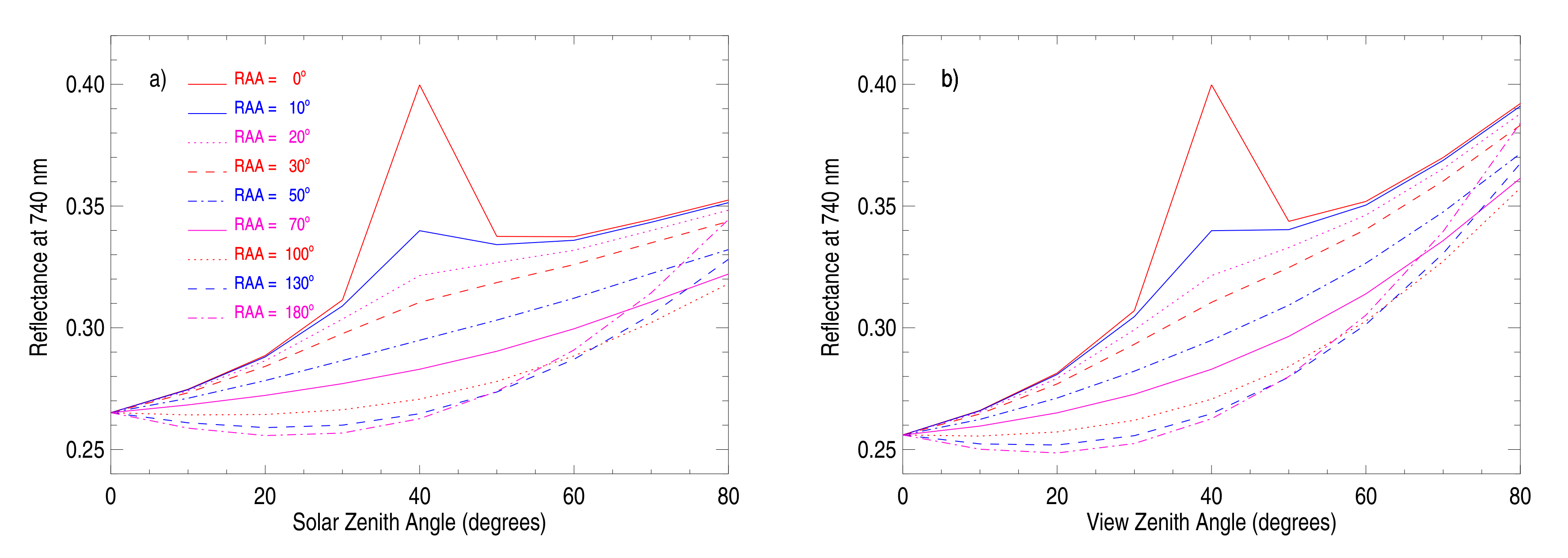
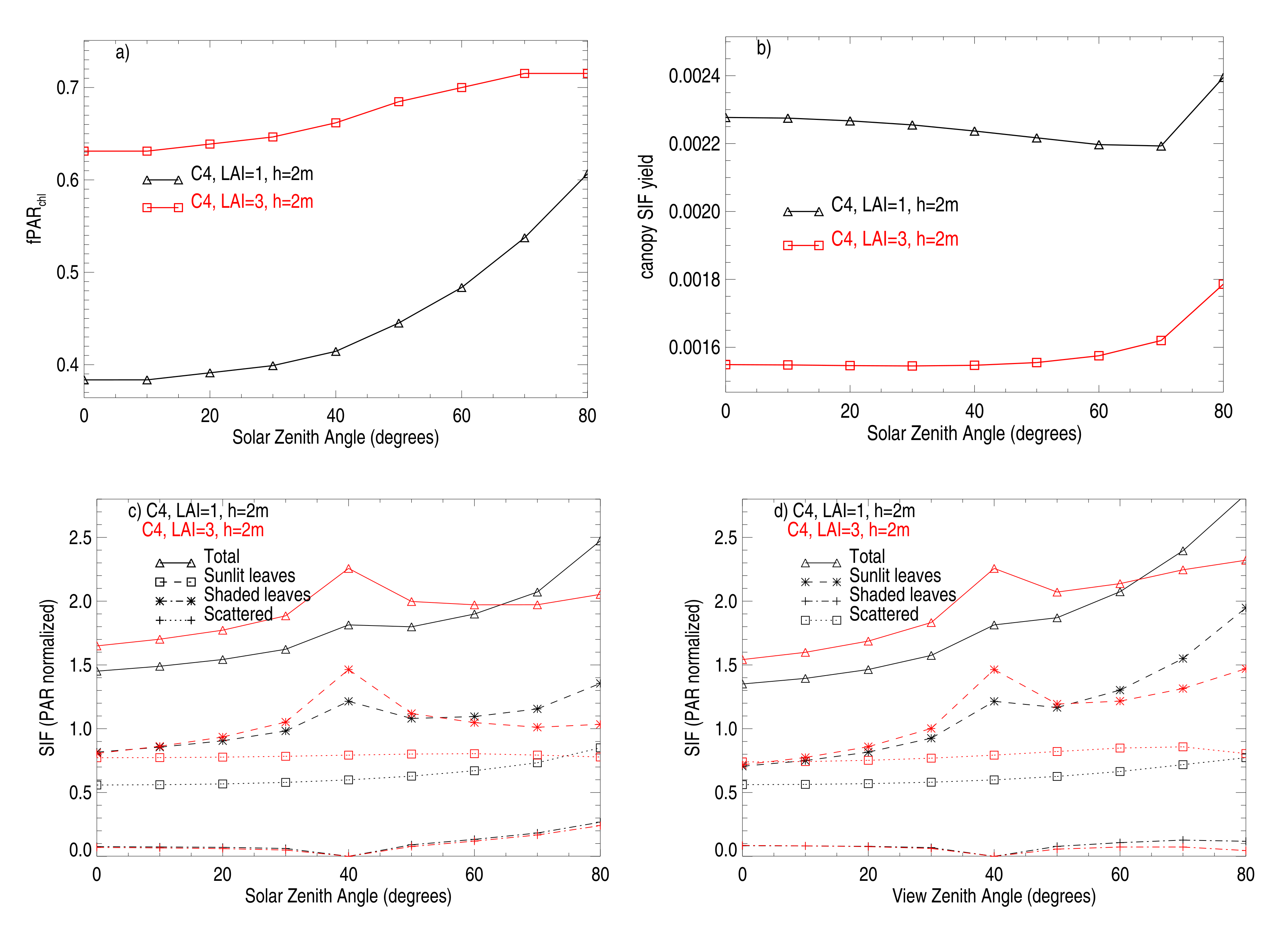
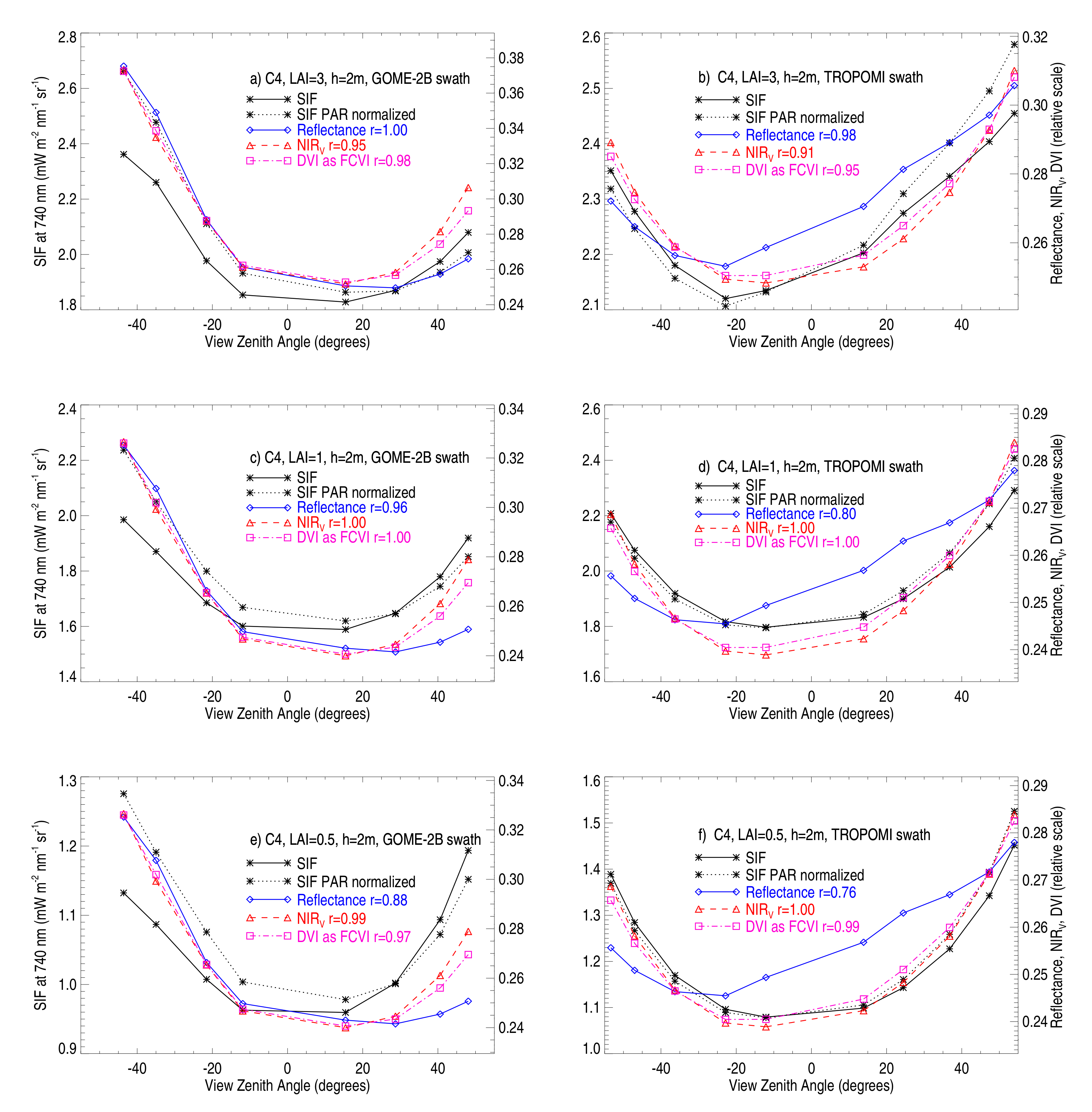
3.2. SCOPE Simulations

Figure 8 and Figure 9 show how the components of simulated top of canopy (TOC) SIF in Equation (1) vary with sun–satellite geometry that aid in the interpretation of the GOME-2 and TROPOMI SIF swath dependences. With SCOPE we were able to vary certain angles (e.g., VZA) while holding others (e.g., SZA) constant. We were not able to reproduce these analyses with GOME-2 and TROPOMI owing to the cross-track viewing geometry that varies systematically with SZA. Figure 8 shows SCOPE simulations of various radiation- and canopy-related parameters in Equation (1) that vary only as a function of SZA for the C4 canopy simulation with LAI = 3. APAR variations with SZA are dominated by PAR rather than fPAR.
Figure 8b shows the wavelength-integrated canopy SIF yield, defined as observed total SIF divided by APAR. A SIF emission efficiency factor, defined as the hemispherically averaged SIF at 740 nm divided by APAR chl , is also shown in Figure 8b. Both quantities are normalized by their maximum values. These show a very similar SZA dependence with the highest values at high SZAs. However, there is little diurnal variation in the simulated canopy SIF yield or emission efficiency through a large range of irradiances (SZA < ∼50 ).
Figure 9 shows for the same setup a SIF directional escape factor at 740 nm (i.e., in the direction of the observer), defined as TOC SIF at 740 nm divided by SIF emitted by all photosystems at 740 nm normalized by π . This quantity is shown as a function of SZA at a constant VZA (40 ) and as a function VZA for a constant SZA (40 ) for a range of RAA from 0 to 180 . The hemispherically averaged SIF divided by the SIF emitted by all photosystems is also shown with heavy black lines and only varies with SZA. The hot spot is visible at angles of 40 for the curves at or near the principal plane (e.g., the red solid line for the principal plane). The SIF directional escape variation with SZA is relatively small except in the principal plane (red solid curve) near the hot spot. The directional escape factor varies more with VZA, particularly near the hot spot.
Figure 10a shows for the same setup TOC SIF simulations as a function of SZA for VZA = 40 for the same range of RAA as in Figure 9. The TOC SIF variation with SZA is dominated by that of APAR. Figure 10b similarly shows TOC SIF as a function of VZA at SZA = 40 that is related to the escape factor.
Figure 11a shows simulated TOC SIF normalized by PAR (to a value of incident PAR equivalent to that at 45 SZA) as a function of SZA. PAR normalized SIF generally increases with SZA in contrast with the unnormalized SIF. This dependence is a result of the increasing fPAR and SIF yield with SZA as shown in Figure 10. Figure 11b shows how much of the total PAR normalized TOC SIF is coming from sunlit leaves, shaded leaves, and SIF scattered within the canopy. Here, we see that only a small fraction comes from shaded leaves and of the remainder, it is split similarly between scattered SIF and SIF from sunlit leaves, with an expected peak in SIF from sunlit leaves at the hotspot and a corresponding drop to zero from shaded leaves at the hotspot.
Figure 12a,b similarly shows SCOPE simulated TOC reflectance at 740 nm as a function of SZA and VZA as in Figure 10. This shows that SIF/PAR and 740 nm reflectance have similar geometrical dependence, both with a depicted hot spot.
Figure 13 shows how SIF/PAR and its components vary with LAI for the C4 setup. For the LAI = 1 case, fPAR chl is lower but increases more rapidly with SZA, producing a larger SZA dependence. The canopy yield is higher overall for the LAI = 1 case but has a similar SZA dependence as LAI = 3. SIF/PAR has a larger dependence on VZA and SZA for the LAI = 1 case. The larger VZA dependence for LAI = 1 is due to the effect of seeing more leaves and less ground at high VZA that is more important for lower LAI values. The magnitude of SIF from the sunlit leaves is similar in both cases but there is more scattered SIF from the LAI = 3 canopy. This leads to higher SIF for the LAI = 3 case in general as may be expected, though not at the highest SZAs and VZAs. Similar differences between the deeper canopy C3 LAI = 5 and LAI = 1 cases are shown in Figure A3.
Figure 14 shows SCOPE simulations of TOC SIF, SIF/PAR, R NIR , NIR V , and DVI as a function of VZA for SZAs and phase angles corresponding to typical swath sun–satellite geometries for GOME-2 and TROPOMI; VZAs with negative values correspond to the west sides of the satellite swaths. SCOPE calculations computed at 10 SZAs, 10 VZAs, and 19 RAAs were interpolated to the average geometries shown in Figure 3 for grasslands in the 30–40 latitude band corresponding to June 2018. TOC SIF is shown with and without normalization for incoming PAR. The PAR normalization produces cross-track SIF variations that are more similar to that of reflectance and reflectance-based indices for GOME-2, but overall PAR normalization does not much change the cross-track SIF variation. Similar cross-track behavior of SIF/PAR and reflectance-based indices are shown for the C4 case for geometries corresponding to the 50–60 latitude band in Figure A4 and for the deeper canopy C3 LAI = 5 and LAI = 1 cases in Figure A5.

4. Discussion

4.1. Comparison of GOME-2 and TROPOMI SIF

That the GOME-2 and TROPOMI SIF values overlap (to nearly within estimated uncertainties) when viewing conditions are similar (at the highest latitudes) provides confidence in the consistency of the relative calibration and retrievals from the two satellite-based instruments. It should be noted that the satellites do not sample the Earth in the same way; TROPOMI has greater sampling in general owing to smaller pixels that tend to have less cloud contamination. Also, TROPOMI, with its wider swath can provide greater sampling at the highest latitudes. It should also be noted that NIR reflectances from GOME-2 and TROPOMI are not reported at the same wavelength; GOME-2 reflectance is reported near 780 nm while TROPOMI reflectance is computed across its fitting window near 740 nm. This may contribute some of the differences in behaviors of SIF and reflectance between the two satellites.

4.2. Geometrical Dependencies of SIF and Reflectance

The SCOPE simulated variation in SIF from nadir to a VZA of −45 is substantial at ∼40% for the LAI = 3 case for the GOME-2 geometries and less so for the simulated TROPOMI swath and for the LAI = 1 and LAI = 0.5 cases as seen in Figure 14. The LAI = 1 and LAI = 0.5 cases show a distinctly more symmetric bowl-like cross-track dependence similar to that seen in the TROPOMI data for grasslands, particularly at the higher latitudes (above 40 N). From these simulations, LAI is shown to be an important factor in determining the cross-track SIF dependence in the satellite data. We note here again that the 1D SCOPE model may not capture all of the complexity in a 3D canopy as observed from satellite and the current version does not allow for inhomogeneity in the vertical structure.
Substantial cross-track asymmetry in both observed SIF/PAR and reflectance is shown for the deeper canopy forest PFTs that tend to have higher SIF/PAR and reflectances related to higher LAI values. For some of these canopies (forested) with particularly high SIF/PAR and reflectance, we can also see a well defined hot spot in both SIF and reflectance. This is particularly the case at the middle latitudes as phase angles approach zero. For TROPOMI, the hot spot occurs on the right (East) part of the swath and produces a peak in the cross-track SIF and reflectance (see for example, Figure 2 and Figure 7 for woody savanna and deciduous broadleaf, respectively, at latitudes between 30 N and 50 N). For GOME-2, the hotspot occurs near the western most edge of the swath, leading to a high degree of asymmetry across its swath for these PFTs and latitudes. This is generally captured in the SCOPE simulations (Figure 14a,c).
A bowl-like cross-track pattern that corresponds roughly to VZA with less asymmetry is observed by GOME-2 and TROPOMI for croplands, grasslands, and evergreen needleleaf forests. This variation is particularly apparent at the higher latitudes where SIF values tend to be lower in general, corresponding to lower values of LAI. This is explained by scattering processes affecting both SIF and reflected light within the canopy (i.e., mutual shadowing) and by the bidirectional gap fraction [37,46,70] and is captured in the SCOPE simulations (Figure 14a,c).
SCOPE simulations show that SIF/PAR, R NIR , NIR V , and DVI should all share a similar cross-track dependence for satellite instruments, particularly at higher values of LAI ( 1 < LAI < 5 ). However, SCOPE simulations also show that the SIF/PAR and R NIR cross-track variations begin to diverge at lower LAI values (0.5). For example, correlations between SIF/PAR and R NIR are near to one for LAI = 3 in Figure 14 but drop below 0.9 for the LAI = 0.5 case. The similarities between SIF/PAR and R NIR were explained by (e.g., Yang and van der Tol [39]) through the relationship between canopy scattering of SIF and reflectance (see also e.g., [43,44]). This relationship may be straight-forward under certain conditions that are more likely to hold for far-red SIF examined here than for SIF at red wavelengths. Derivations of straight-forward SIF-reflectance relationships are generally developed under the condition of “black soil”. In reality, soil (as well as other non-green components of the canopy such as woody branches) has a direct contribution to the observed reflectance through the single scattering effects, but does not directly contribute to SIF as long as the soil is not fluorescing (e.g., Yang and van der Tol [39], Colombo et al. [49]). The derived straight-forward relationship between canopy scattering of SIF and reflectance therefore will start to break down with increasing gap fraction. SCOPE simulations of NIR V and DVI show higher correlations with SIF/PAR, consistent with results of Zeng et al. [44] and Yang et al. [25].
This aspect of the SCOPE simulations is generally consistent with the observed correspondence (or lack thereof) between SIF/PAR, R NIR , NIR V , and DVI across the tracks of GOME-2 and TROPOMI. GOME-2 and TROPOMI measurements show similar cross-track behavior of SIF/PAR, R NIR , NIR V , and DVI for the deciduous broadleaf forests in Figure 7 and croplands with DVI values > ∼0.12 (typical for latitudes > 30N) in Figure 4. In contrast, TROPOMI and GOME-2 observations show more mixed results for cross-track correlations between SIF/PAR and reflectance-based parameters for grasslands and other PFTs that display lower values of SIF/PAR and DVI.
There are generally larger differences between SIF and reflectance for GOME2 and TROPOMI measurements than in SCOPE simulations. In addition, neither DVI nor NIR V has consistently higher correlations with SIF/PAR, particularly at lower values of DVI corresponding to lower LAI canopies. There are several possible explanations. We note that SCOPE simulates a homogeneous canopy, i.e., LAI is distributed evenly within a simulated scene. Therefore, the contribution of the directly scattered light from the soil surface to the reflectance is typically underestimated for sparse vegetation or scenes with larger gap fractions. While SCOPE would produce a larger divergence between SIF and reflectance at even lower LAI values (<0.5), the gap fraction would still likely be underestimated for inhomogeneous vegetation. It should also be noted that reflectances are more sensitive than SIF to the effects of clouds [69], and this could lead to some of the differences between the cross-track variations of SIF/PAR and reflectance-based indices. In addition, there may still be residual biases in the SIF/PAR retrievals as the signal to noise ratios are fairly low. Three dimensional effects that are not captured by SCOPE may play a role. Finally, we note that there could be variations in SIF yield as a function of local solar time (illumination). SCOPE simulations generally do not support that the large cross-track differences between SIF/PAR and reflectances for lower LAI scenes would result from SIF yield variations across the track.
Differences in the geometrical dependences of observed SIF/PAR and reflectance-based indices appear to be substantial in many cases corresponding to low DVI or LAI values. This is a concern for methods that rely upon reflectance or reflectance-based indices to normalize geometrical variations in SIF observations from wide swath instruments to estimate a more intrinsic property of SIF, such as SIF emitted at the photosystem level. While some approaches attempt to address the issue of soil reflectance (e.g., [43,44,45]), it is not clear to what extent and under which conditions these methodologies applied to satellite data can provide the needed accuracies for various applications. Yang et al. [25] found that FCVI, NIR V , and FCVI × NDVI (an attempt to improve upon FCVI to better account for soil effects) all showed errors in approximating Γ rt in the most challenging cases of sparse canopies with low LAI with SCOPE simulations. They suggest that errors of less than 30% could be obtained for cases of FCVI > 0.18. Our results are generally consistent with these conclusions. Further work is needed to evaluate these methods with satellite data under a variety of conditions including at different spatio-temporal scales. One method of evaluating such approaches will be to examine the resulting cross-track dependences of the derived intrinsic SIF components (for example normalizing SIF by PAR and fPAR). Averaging over and across large regions, as done here, is needed to mitigate the effect of retrieval noise, which is large even for the highest quality satellite SIF data currently available.
Ground-based measurements over various canopies at different geometries also show different bidirectional distributions of SIF including asymmetric bowl-like patterns for erectophile and spherical canopies and a more dome-like shape with a peak at the hotspot for phanophile canopy types [37,46]. These measurements showed varied amounts of correlation between SIF and NIR reflectance. Our satellite measurements for high LAI canopies are generally consistent with these observations. Biriukova et al. [46] also performed SCOPE simulations and showed that the bidirectionality of SIF is mainly controlled by the leaf inclination distribution function (LIDF); the magnitude and shape of the hotspot is controlled by the LAI and the ratio of leaf width to canopy height, with low ratios and high LAI leading to a stronger and more pronounced hotspot, as is present in our satellite measurements of deciduous broadleaf and mixed forests.
In summary, our analysis of GOME-2 and TROPOMI data show that for very dense canopies such as deciduous broadleaf forests and mature croplands, R NIR , NIR V , and DVI all show a very similar cross-track patterns as SIF/PAR. We are not able to discern if any of these reflectance-based indices provides a superior approximation of Γ rt . For sparse and even some moderately-vegetated canopies, the cross-track behavior of all of these parameters diverges substantially from that of SIF/PAR, in contrast to the SCOPE simulations. It is unclear how well the reflectance-based indices will work for scenarios in between these two extremes and if a single threshold value derived from the reflectances will apply generally. The fluorescence yield ( Φ F in Equation (1)) should be PAR dependent and different for sunlit and shaded leaves. As Φ F also varies with stress, the SIF yield derived for a particular geometry may vary from the canopy SIF yield. This may contribute to the differences between cross-track SIF and reflectance observations and 1D simulations and needs to be considered for interpretation of directional SIF.

4.3. Implications for the Use of Time Series of Gridded Averages from Large Swath Sensors

Many studies have utilized time series of gridbox SIF averages from wide-swath sensors including GOME-2 to investigate interannual variations such as the effects of drought (e.g., [13,71,72]). Our analysis of GOME-2 and TROPOMI SIF data indicates that some of the day-to-day SIF variability for a given location arises from daily changes in the illumination and viewing geometry as the orbits of host satellites do not follow a common ground track every day. The use of time-series of gridded SIF data from such sensors is valid so long as there is adequate and consistent sampling over the swath throughout the record of interest. This is generally the case for monthly data from GOME-2; a typical 0.5 gridbox over a month encompasses about 10–20 samples. Higher spatial and/or temporal resolution averages would be appropriate for TROPOMI.
One change in sampling of a long record SIF data set occurs with the GOME-2A (on MetOp-A); its observing mode changed from the nominal large swath to a reduced swath with smaller pixels in July 2013. To assess the impact of the change in sampling, we computed gridded SIF monthly means with GOME-2B using all swath positions and using only those with VZA < 35 similar to the small swath mode GOME-2A. The GOME-2B swath is the same width as that of GOME-2A in its earlier observation mode. The bias between the two samples is very small (restricted VZA averages lower by 0.02 mW m 2 nm 1 sr 1 , see Figure A6). This provides some confidence in time series analyses of monthly mean gridded data with GOME-2A (biases due to instrument degradation not withstanding).
Zhang et al. [40] pointed out that caution should be applied when using SIF from the various observation modes of the Orbiting Carbon Observatory 2 (OCO-2) that have different samplings of VZAs (not necessarily symmetric about the nadir view). Our results with TROPOMI span the range of observing conditions of OCO-2 and agree with the findings of Zhang et al. [40] that the different geometries sampled by the three observation modes (nadir, glint, and target) should produce systematic differences in SIF. The general caution on the use of different observing modes for scientific studies, supported by our results, also applies to OCO-3 as well as GOSAT; the latter underwent a change in its cross-track swath sampling during the mission.

5. Conclusions

We have shown that for low Earth orbit (LEO) sensors measuring far-red SIF, variations of sun–satellite geometry across the satellite swath are also related to local solar time of the observation, making it difficult to disentangle physiological effects, including those related to diurnal variations in light-use efficiency, from sun–satellite geometry effects. We show that there are substantial systematic variations in far-red SIF across the satellite swaths of GOME-2 and TROPOMI related to sun-sensor geometry and that these variations differ according to canopy properties, in particular the LAI. The variations are roughly consistent with those predicted using the SCOPE canopy radiative transfer model as well as previous ground-based measurements. SIF tends to increase with decreasing phase angle and increasing VZA and SZA. Cross track variations in SIF/PAR are highly correlated with R NIR , NIR V , and DVI for dense canopies such as deciduous broadleaf forests near the summer solstice and crops in a mature state as predicted by SCOPE simulations. This is encouraging as these parameters have been proposed as a means to account for the angular dependencies of SIF in order to extract the embedded physiological information. However, the observed differences in cross-track dependences of SIF are not well captured with any of the reflectance-based indices for sparsely vegetated canopies as well as some moderately vegetated canopies. We note that the physiological status of the vegetation is unknown, and this may affect the cross track correlations shown here as well. More testing of these methods needs to be applied to satellite- as well as ground-based data under a variety of conditions in order to develop reliable thresholds for which the proposed approaches would be applicable. We recommend that both NIR and red wavelength reflectances be provided with satellite SIF data sets if possible for further studies. We find that GOME-2 and TROPOMI far-red SIF values agree to nearly within their estimated uncertainties where their sun–satellite geometries are similar (high northern latitudes in summer). We also note that it is imperative to continue to identify biases and improve bias correction schemes within the SIF retrieval process.
SIF geometrical dependencies will also be important for SIF-capable sensors in geostationary Earth orbit (GEO). Several such sensors are planned to be launched over the next decade including the NASA Earth Ventures Tropospheric Emissions: Monitoring Pollution (TEMPO) and the Geostationary Carbon Observatory (GeoCarb) as well as the ESA Sentinel 4 ultraviolet visible near-infrared (UVN) sounder [73]. These sensors will face a different scenario as compared with those in LEO. For GEO sensors, VZAs at a given point on the ground will be fixed, while the SZA will change throughout the day. A significant portion of the GEO coverage will have moderate to high VZAs (latitudes higher than ∼30 ) [74] where the SIF dependence on SZA and phase angle will be substantial. There will also be a need to connect SIF measurements from the different GEO instruments as well as the GEO measurements from a single sensor at different locations and thus with different VZAs. SIF measurements from LEO will be helpful in this respect provided that the sun-sensor geometry can be accurately accounted for.

Author Contributions

Conceptualization, J.J. and Y.Y.; Methodology: J.J., Y.Y., C.v.d.T., P.Y., P.K., C.F., Y.S.; Software, J.J., Y.Y., C.v.d.T., P.Y., P.K., C.F., and L.G.; Formal analysis, J.J., Y.Y., P.Y., C.v.d.T., and P.C.; Investigation: J.J., Y.Y., C.v.d.T., and P.Y.; Visualization: J.J., Y.Y., C.v.d.T, and P.Y.; Writing—Original Draft Preparation: J.J. and Y.Y.; Writing—Review & Editing, J.J., Y.Y., C.v.d.T., P.Y., P.K., C.F., P.C., Y.S., L.G., and N.P.; Project Administration: N.P.; Funding Acquisition: N.P., C.F., P.K., J.J., Y.S.,and C.v.d.T.; Data Curation: J.J., P.K. and C.F. All authors have read and agreed to the published version of the manuscript.

Funding

This work was supported by the NASA Making Earth System Data Records for Use in Research Environments (MEaSUREs), Earth Science US Participating Investigator (ESUSPI), and Arctic-Boreal Vulnerability Experiment (ABoVE) and Multi-Source Land Imaging (MuSLI) programs, specifically grants ABoVE 80NSSC19M0110 and MuSLI 80NSSC18K0337. PY was funded by the Netherlands Organization for Scientific Research (NWO), project ALWGO.2018.018.

Acknowledgments

We thank EUMETSAT and ESA for making possible the distribution of the high quality GOME-2 and TROPOMI data sets, respectively, used in this study.

Conflicts of Interest

No potential conflict of interest was reported by the authors.The founding sponsors had no role in the design of the study; in the collection, analyses, or interpretation of data; in the writing of the manuscript, and in the decision to publish the results.

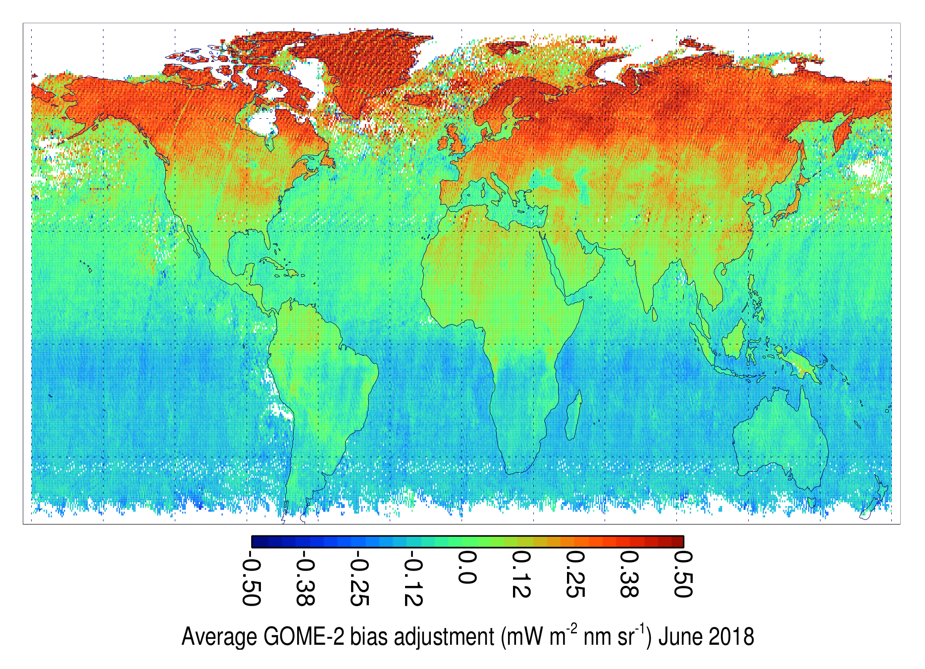
Appendix A. Neural Network Based GOME-2 Bias Adjustment

We implemented a new scheme for addressing biases in GOME-2 retrievals identified by Köhler et al. [55] as an update to that used in Joiner et al. [59]. The approach uses a three layer feed forward neural network that was constructed by trial and error within the interactive data language (IDL) set of routines. Both inputs and outputs were first scaled to produce a mean of zero and a standard deviation of unity. The activation function for the first layer is the so-called soft-sign, i.e.,
f ( x ) = x 1 + | x | ,
and for the second layer is a logistic function, i.e.,
f ( x ) = 1 1 + x x ,
and for the third layer was the so-called bent identity, i.e.,
f ( x ) = x 2 + 1 1 2 + x .
We used an adaptive moment estimation optimizer to minimize the error function with a learning rate of 0.1 and default values of β 1 and β 2 , parameters used by the algorithm (0.9 and 0.999, respectively). The main advantage of the neural network for bias correction is that it eliminated small discontinuities along latitude lines used as boundaries in the regression approach of Joiner et al. [59].
Figure A1 shows averaged SIF (gridded) bias adjustments computed for June 2018. The bias is seen to have a strong latitudinal gradient. Bias adjustments are larger on average over land in the northern hemisphere owing to higher average reflectances, particularly for Greenland.
Figure A1. Mean GOME-2 SIF bias corrections on a grid of 0.5 latitude by 0.5 longitude for the month of June 2018 using observations with effective cloud fractions < 0.3.
Remotesensing 12 02346 g0a1

Appendix B. Details of SCOPE Simulation

Table A1 provides a list of parameters used in the SCOPE model for the simulations shown in Section 3.2.
Table A1. Listing of SCOPE input parameters.
ParameterValueValueUnitDescription
PROSPECTC4C3
Cab7080 μ g cm 2 Chlorophyll AB content
Cca20 μ g cm 2 Carotenoid content
Cdm0.012 μ g cm 2 Dry matter content
Cw0.009 cmleaf water equivalent layer
Cs0 fractionsenescent material fraction
Cant0 μ g cm 2 Anthocyanins
N1.4 leaf thickness parameters
ρ thermal 0.01 broadband thermal reflectance
τ thermal 0.01 broadband thermal transmittance
Leaf_Biochemical
Vcmo6080 μ mol m 2 s 1 maximum carboxylation capacity
m8 stomatal conductance parameter
BallBerry00.01
Type10 Photochemical pathway: 0 = C3, 1 = C4
kV0.6396 extinction coefficient for Vcmax in the vertical
Rdparam0.015 Respiration = Rdparam*Vcmcax
Tyear15 Cmean annual temperature
beta0.507 fraction of photons partitioned to PSII
kNPQs0 s 1 rate constant of sustained thermal dissipation
qLs1 fraction of functional reaction centres
stressfactor1 stress factor to reduce Vcmax
Fluorescence
fqe0.01 fluorescence quantum yield efficiency at photosystem level
Soil
spectrumBSM1 Spectrum name or number
rss500 s m 1 soil resistance for evaporation from the pore space
rs thermal 0.06 thermal broadband soil reflectance (1- ϵ )
csl1.18E+03 J kg 1 K 1 specific heat capacity of the soil
rhosl1.80E+03 kg m 3 specific mass of the soil
lambdas1.55 J m 1 K 1 heat conductivity of the soil
SMC0.25 volumetric soil moisture content in the root zone
BSMBrightness0.5 soil brightness
BSMlat25 latitude
BSMlon45 longitude
Canopy
LAI1.31.5m 2 m 2 Leaf area index
hc230mvegetation height
LIDFa−0.35 leaf inclination
LIDFb−0.15 variation in leaf inclination
leafwidth0.2 mleaf width
Meteo
z1040mmeasurement height of meteorological data
Rin600 W m 2 broadband incoming shortwave radiation (0.4–2.5 μ m)
Ta20 Kair temperature
Rli300 W m 2 broadband incoming longwave radiation (2.5–50 μ m)
p970 hPaair pressure
ea15 hPaatmospheric vapor pressure
u2 m s 1 wind speed at height z
Ca380 ppmatmospheric CO 2 concentration
Oa209 per milleatmospheric O 2 concentration
Aerodynamic
zo0.2463.69mroughness length for momentum of the canopy
d1.3420.1mdisplacement height
Cd0.3 leaf drag coefficient
rb10 s m 1 leaf boundary resistance
CR0.35 Drag coefficient for isolated tree
CD120.6 fitting parameter
Psicor0.2 Roughness layer correction
CSSOIL0.01 Drag coefficient for soil
rbs10 s m 1 soil boundary layer resistance
rwc0 s m 1 within canopy layer resistance
Figure A2 shows three different methods of computing a solar zenith angle dependence within SCOPE. In the first simulation (blue line), the magnitude of the irradiance remains the same for all simulations, while the incident angle changes. The adjustment to the appropriate magnitude of irradiance was applied to the SCOPE-modelled SIF afterwards. In this scenario, SCOPE runs with an SZA-independent irradiance, and thus variations of Φ F due to irradiance were not accounted for by the model. This is what was done in the simulations shown in the main part of the paper. We tested the accuracy of this approach with two other simulations. The pink curve shows results when the magnitude of the irradiance was adjusted to the appropriate SZA before input into SCOPE. In this scenario, the model also simulates variations in Φ F due to SZA. This somewhat reduces the sensitivity to SZA, because the model predicts a lower Φ F when irradiance is high. However, the difference is not large, and this also suggests that there is not much signal of diurnal variation in Φ F in canopy level SIF. The black line shows SCOPE results using separate MODTRAN simulations (for a given aerosol loading, etc.) for each SZA as input to SCOPE instead of correcting the magnitude (with cosine of the SZA). This takes into account the fact that the contribution of diffuse radiation also changes with SZA. This has an even smaller effect than whether a correction is made to either inputs or outputs.
Figure A2. Three different approaches to account for the SIF solar zenith angle dependence in SCOPE showing very little differences in the approaches (see text for more details). In these simulations, the viewing geometry was nadir.
Remotesensing 12 02346 g0a2
Figure A3 and Figure A5 show SCOPE simulation results for the C3 setup, contrasting results for LAI = 1 and LAI = 5 cases. These figures have counterparts for the C4 setup in the main part of the paper and show similar differences between high and lower LAI cases. For example, the hotspot effect is smaller for the LAI = 1 case, but the VZA and SZA dependences are generally larger as shown in Figure A3, similar to those shown in Figure 13. The C3 cross-track dependence, shown in Figure A5 displays less asymmetry for the LAI = 1 case, similar to what was shown for C4 in Figure 14.
Figure A3. SCOPE simulations for the C3 setup comparing results for LAI = 5 and LAI = 1; (a) fPAR chl ; (b) wavelength integrated SIF yield; decomposition of total normalized SIF into that from sunlit leaves, shaded leaves, and from SIF scattered within the canopy as a function of (c) solar zenith angle and (d) view zenith angle.
Remotesensing 12 02346 g0a3
Figure A4. Similar to Figure 14 but for satellite geometry at 50–60 N; SCOPE simulations of SIF and reflectance for the C4 setup to mimic typical sun-sensor geometry across a swath (shown as a function of view zenith angle but at each angle for appropriate values of solar zenith angle and phase angle corresponding to the geometry for 50–60 N in June for LAI = 3: (a) GOME-2B and (b) TROPOMI; LAI = 1: (c) GOME-2B and (d) TROPOMI; and LAI = 0.5: (e) GOME-2B and (f) TROPOMI. SIF PAR normalized shows SIF normalized to a constant solar zenith angle representative of the center of the swath.
Remotesensing 12 02346 g0a4
Figure A5. Similar to Figure 14 but for the C3 setup; SCOPE simulations of SIF and reflectance for the C3 setup to mimic typical sun-sensor geometry across a swath (shown as a function of view zenith angle but at each angle for appropriate values of solar zenith angle and phase angle corresponding to the geometry for 30–40 N in June for LAI = 5: (a) GOME-2B (left) and (b) TROPOMI (right); and LAI = 1: (c) GOME-2B (left) and (d) TROPOMI (right). SIF PAR normalized shows SIF normalized to a constant solar zenith angle representative of the center of the swath.
Remotesensing 12 02346 g0a5

Appendix C. Monthly Means from GOME-2B with Different Samplings of VZA

To check whether the change in operations of GOME-2A from nominal to small swath mode in July 2013 produces a bias in the time series, we examined one month of GOME-2B data where we gridded the values using all swath positions versus only those pixels with VZA < 35 . The results are shown in Figure A6. The overall bias between the two different sampling schemes is very small. Therefore, the change in GOME-2 operations is not expected to cause substantial discontinuities in gridded SIF time series. None-the-less, the change in observation mode, leading to changes in swath width and viewing angles, should be mentioned when using GOME-2A time series SIF data for scientific studies.
Figure A6. Two dimensional histogram of monthly gridded means of SIF (data from August 2013) for gridboxes with monthly average using all data of >0.1 mW m 2 nm 1 sr 1 ; colors represent the number of gridboxes in a bin. The bias of 0.02 is computed as the mean difference between all data and data with VZA < 35 .
Remotesensing 12 02346 g0a6

References

  1. Meroni, M.; Rossini, M.; Guanter, L.; Alonso, L.; Rascher, U.; Colombo, R.; Moreno, J. Remote sensing of solar-induced chlorophyll fluorescence: Review of methods and applications. Remote Sens. Environ. 2009, 113, 2037–2051. [Google Scholar] [CrossRef]
  2. Mohammed, G.H.; Colombo, R.; Middleton, E.M.; Rascher, U.; van der Tol, C.; Nedbal, L.; Goulas, Y.; Pérez-Priego, O.; Damm, A.; Meroni, M.; et al. Remote sensing of solar-induced chlorophyll fluorescence (SIF) in vegetation: 50 years of progress. Remote Sens. Environ. 2019, 231, 111177. [Google Scholar] [CrossRef]
  3. Guanter, L.; Zhang, Y.; Jung, M.; Joiner, J.; Voigt, M.; Berry, J.A.; Frankenberg, C.; Huete, A.R.; Zarco-Tejada, P.; Lee, J.E.; et al. Global and time-resolved monitoring of crop photosynthesis with chlorophyll fluorescence. Proc. Natl. Acad. Sci. USA 2014, 111, E1327–E1333. [Google Scholar] [CrossRef] [PubMed] [Green Version]
  4. Joiner, J.; Yoshida, Y.; Vasilkov, A.P.; Schaefer, K.; Jung, M.; Guanter, L.; Zhang, Y.; Garrity, S.; Middleton, E.M.; Huemmrich, K.F.; et al. The seasonal cycle of satellite chlorophyll fluorescence observations and its relationship to vegetation phenology and ecosystem atmosphere carbon exchange. Remote Sens. Environ. 2014, 152, 375–391. [Google Scholar] [CrossRef] [Green Version]
  5. Parazoo, N.C.; Bowman, K.; Fisher, J.B.; Frankenberg, C.; Jones, D.B.A.; Cescatti, A.; Pérez-Priego, O.; Wohlfahrt, G.; Montagnani, L. Terrestrial gross primary production inferred from satellite fluorescence and vegetation models. Glob. Chang. Biol. 2014, 20, 3103–3121. [Google Scholar] [CrossRef] [PubMed]
  6. Zhang, Y.; Xiao, X.; Jin, C.; Dong, J.; Zhou, S.; Wagle, P.; Joiner, J.; Guanter, L.; Zhang, Y.; Zhang, G.; et al. Consistency between sun-induced chlorophyll fluorescence and gross primary production of vegetation in North America. Remote Sens. Environ. 2016, 183, 154–169. [Google Scholar] [CrossRef] [Green Version]
  7. Sun, Y.; Frankenberg, C.; Wood, J.D.; Schimel, D.S.; Jung, M.; Guanter, L.; Drewry, D.T.; Verma, M.; Porcar-Castell, A.; Griffis, T.J.; et al. OCO-2 advances photosynthesis observation from space via solar-induced chlorophyll fluorescence. Science 2017, 358, eaam5747. [Google Scholar] [CrossRef] [Green Version]
  8. Liu, L.; Guan, L.; Liu, X. Directly estimating diurnal changes in GPP for C3 and C4 crops using far-red sun-induced chlorophyll fluorescence. Agric. For. Meteorol. 2017, 232, 1–9. [Google Scholar] [CrossRef]
  9. Li, X.; Xiao, J.; He, B.; Altaf, A.M.; Beringer, J.; Desai, A.R.; Emmel, C.; Hollinger, D.Y.; Krasnova, A.; Mammarella, I.; et al. Solar-induced chlorophyll fluorescence is strongly correlated with terrestrial photosynthesis for a wide variety of biomes: First global analysis based on OCO-2 and flux tower observations. Glob. Chang. Biol. 2018, 24, 3990–4008. [Google Scholar] [CrossRef]
  10. Wieneke, S.; Burkart, A.; Cendrero-Mateo, M.; Julitta, T.; Rossini, M.; Schickling, A.; Schmidt, M.; Rascher, U. Linking photosynthesis and sun-induced fluorescence at sub-daily to seasonal scales. Remote Sens. Environ. 2018, 219, 247–258. [Google Scholar] [CrossRef]
  11. Damm, A.; Guanter, L.; Paul-Limoges, E.; van der Tol, C.; Hueni, A.; Buchmann, N.; Eugster, W.; Ammann, C.; Schaepman, M. Far-red sun-induced chlorophyll fluorescence shows ecosystem-specific relationships to gross primary production: An assessment based on observational and modeling approaches. Remote Sens. Environ. 2015, 166, 91–105. [Google Scholar] [CrossRef]
  12. Zhang, Y.; Guanter, L.; Berry, J.A.; van der Tol, C.; Yang, X.; Tang, J.; Zhang, F. Model-based analysis of the relationship between sun-induced chlorophyll fluorescence and gross primary production for remote sensing applications. Remote Sens. Environ. 2016, 187, 145–155. [Google Scholar] [CrossRef] [Green Version]
  13. Ma, X.; Huete, A.; Cleverly, J.; Eamus, D.; Chevallier, F.; Joiner, J.; Poulter, B.; Zhang, Y.; Guanter, L.; Meyer, W.; et al. Drought rapidly diminishes the large net CO2 uptake in 2011 over semi-arid Australia. Sci. Rep. 2016, 6, 37747. [Google Scholar] [CrossRef]
  14. Alden, C.B.; Miller, J.B.; Gatti, L.V.; Gloor, M.M.; Guan, K.; Michalak, A.M.; Laan-Luijkx, I.T.; Touma, D.; Andrews, A.; Basso, L.S.; et al. Regional atmospheric CO2 inversion reveals seasonal and geographic differences in Amazon net biome exchange. Glob. Chang. Biol. 2016, 22, 3427–3443. [Google Scholar] [CrossRef] [PubMed]
  15. Green, J.K.; Konings, A.G.; Alemohammad, S.H.; Berry, J.; Entekhabi, D.; Kolassa, J.; Lee, J.E.; Gentine, P. Regionally strong feedbacks between the atmosphere and terrestrial biosphere. Nat. Geosci. 2017, 10, 410–414. [Google Scholar] [CrossRef] [PubMed]
  16. Madani, N.; Kimball, J.S.; Jones, L.A.; Parazoo, N.C.; Guan, K. Global analysis of bioclimatic controls on ecosystem productivity using satellite observations of solar-induced chlorophyll fluorescence. Remote Sens. 2017, 9, 530. [Google Scholar] [CrossRef] [Green Version]
  17. Köhler, P.; Guanter, L.; Kobayashi, H.; Walther, S.; Yang, W. Assessing the potential of sun-induced fluorescence and the canopy scattering coefficient to track large-scale vegetation dynamics in Amazon forests. Remote Sens. Environ. 2018, 204, 769–785. [Google Scholar] [CrossRef] [Green Version]
  18. Berkelhammer, M.; Stefanescu, I.C.; Joiner, J.; Anderson, L. High sensitivity of gross primary production in the Rocky Mountains to summer rain. Geophys. Res. Lett. 2017, 44, 3643–3652. [Google Scholar] [CrossRef]
  19. Luus, K.A.; Commane, R.; Parazoo, N.C.; Benmergui, J.; Euskirchen, E.S.; Frankenberg, C.; Joiner, J.; Lindaas, J.; Miller, C.E.; Oechel, W.C.; et al. Tundra photosynthesis captured by satellite-observed solar-induced chlorophyll fluorescence. Geophys. Res. Lett. 2017, 44, 1564–1573. [Google Scholar] [CrossRef] [Green Version]
  20. Walther, S.; Voigt, M.; Thum, T.; Gonsamo, A.; Zhang, Y.; Köhler, P.; Jung, M.; Varlagin, A.; Guanter, L. Satellite chlorophyll fluorescence measurements reveal large-scale decoupling of photosynthesis and greenness dynamics in boreal evergreen forests. Glob. Chang. Biol. 2016, 22, 2979–2996. [Google Scholar] [CrossRef] [Green Version]
  21. Walther, S.; Guanter, L.; Heim, B.; Jung, M.; Duveiller, G.; Wolanin, A.; Sachs, T. Assessing the dynamics of vegetation productivity in circumpolar regions with different satellite indicators of greenness and photosynthesis. Biogeosciences 2018, 15, 6221–6256. [Google Scholar] [CrossRef] [Green Version]
  22. Monteith, J.L. Solar radiation and productivity in tropical ecosystems. J. Appl. Ecol. 1972, 9, 747–766. [Google Scholar] [CrossRef] [Green Version]
  23. Monteith, J.L. The management of inputs for yet greater agricultural yield and efficiency—Climate and the efficiency of crop production in Britain. Philos. Trans. R. Soc. Lond. B Biol. Sci. 1977, 281, 277–294. [Google Scholar] [CrossRef]
  24. Ač, A.; Malenovský, Z.; Olejníčková, J.; Gallé, A.; Rascher, U.; Mohammed, G. Meta-analysis assessing potential of steady-state chlorophyll fluorescence for remote sensing detection of plant water, temperature and nitrogen stress. Remote Sens. Environ. 2015, 168, 420–436. [Google Scholar] [CrossRef] [Green Version]
  25. Yang, P.; van der Tol, C.; Campbell, P.K.; Middleton, E.M. Fluorescence Correction Vegetation Index (FCVI): A physically based reflectance index to separate physiological and non-physiological information in far-red sun-induced chlorophyll fluorescence. Remote Sens. Environ. 2020, 240, 111676. [Google Scholar] [CrossRef]
  26. Verrelst, J.; Rivera, J.P.; van der Tol, C.; Magnani, F.; Mohammed, G.; Moreno, J. Global sensitivity analysis of the SCOPE model: What drives simulated canopy-leaving sun-induced fluorescence? Remote Sens. Environ. 2015, 166, 8–21. [Google Scholar] [CrossRef]
  27. van der Tol, C.; Rossini, M.; Cogliati, S.; Verhoef, W.; Colombo, R.; Rascher, U.; Mohammed, G. A model and measurement comparison of diurnal cycles of sun-induced chlorophyll fluorescence of crops. Remote Sens. Environ. 2016, 186, 663–677. [Google Scholar] [CrossRef]
  28. Migliavacca, M.; Perez-Priego, O.; Rossini, M.; El-Madany, T.S.; Moreno, G.; van der Tol, C.; Rascher, U.; Berninger, A.; Bessenbacher, V.; Burkart, A.; et al. Plant functional traits and canopy structure control the relationship between photosynthetic CO2 uptake and far-red sun-induced fluorescence in a Mediterranean grassland under different nutrient availability. New Phytol. 2017, 214, 1078–1091. [Google Scholar] [CrossRef] [Green Version]
  29. Yang, K.; Ryu, Y.; Dechant, B.; Berry, J.A.; Hwang, Y.; Jiang, C.; Kang, M.; Kim, J.; Kimm, H.; Kornfeld, A.; et al. Sun-induced chlorophyll fluorescence is more strongly related to absorbed light than to photosynthesis at half-hourly resolution in a rice paddy. Remote Sens. Environ. 2018, 216, 658–673. [Google Scholar] [CrossRef]
  30. Yang, P.; van der Tol, C.; Verhoef, W.; Damm, A.; Schickling, A.; Kraska, T.; Muller, O.; Rascher, U. Using reflectance to explain vegetation biochemical and structural effects on sun-induced chlorophyll fluorescence. Remote Sens. Environ. 2019, 231, 110996. [Google Scholar] [CrossRef]
  31. Porcar-Castell, A.; Tyystjärvi, E.; Atherton, J.; van der Tol, C.; Flexas, J.; Pfündel, E.E.; Moreno, J.; Frankenberg, C.; Berry, J.A. Linking chlorophyll a fluorescence to photosynthesis for remote sensing applications: Mechanisms and challenges. J. Exp. Bot. 2014, 65, 4065–4095. [Google Scholar] [CrossRef] [PubMed]
  32. Celesti, M.; van der Tol, C.; Cogliati, S.; Panigada, C.; Yang, P.; Pinto, F.; Rascher, U.; Miglietta, F.; Colombo, R.; Rossini, M. Exploring the physiological information of Sun-induced chlorophyll fluorescence through radiative transfer model inversion. Remote Sens. Environ. 2018, 215, 97–108. [Google Scholar] [CrossRef]
  33. Wittenberghe, S.V.; Alonso, L.; Verrelst, J.; Moreno, J.; Samson, R. Bidirectional sun-induced chlorophyll fluorescence emission is influenced by leaf structure and light scattering properties, A bottom-up approach. Remote Sens. Environ. 2015, 158, 169–179. [Google Scholar] [CrossRef]
  34. Van der Tol, C.; Verhoef, W.; Timmermans, J.; Verhoef, A.; Su, Z. An integrated model of soil-canopy spectral radiances, photosynthesis, fluorescence, temperature and energy balance. Biogeosciences 2009, 6, 3109–3129. [Google Scholar] [CrossRef] [Green Version]
  35. Guanter, L.; Frankenberg, C.; Dudhia, A.; Lewis, P.E.; Gómez-Dans, J.; Kuze, A.; Suto, H.; Grainger, R.G. Retrieval and global assessment of terrestrial chlorophyll fluorescence from GOSAT space measurements. Remote Sens. Environ. 2012, 121, 236–251. [Google Scholar] [CrossRef]
  36. Cogliati, S.; Verhoef, W.; Kraft, S.; Sabater, N.; Alonso, L.; Vicent, J.; Moreno, J.; Drusch, M.; Colombo, R. Retrieval of sun-induced fluorescence using advanced spectral fitting methods. Remote Sens. Environ. 2015, 169, 344–357. [Google Scholar] [CrossRef]
  37. Liu, L.; Liu, X.; Wang, Z.; Zhang, B. Measurement and analysis of bidirectional SIF emissions in wheat canopies. IEEE Trans. Geosci. Remote Sens. 2016, 54, 2640–2651. [Google Scholar] [CrossRef]
  38. He, L.; Chen, J.M.; Liu, J.; Mo, G.; Joiner, J. Angular normalization of GOME-2 Sun-induced chlorophyll fluorescence observation as a better proxy of vegetation productivity. Geophys. Res. Lett. 2017, 44, 5691–5699. [Google Scholar] [CrossRef]
  39. Yang, P.; van der Tol, C. Linking canopy scattering of far-red sun-induced chlorophyll fluorescence with reflectance. Remote Sens. Environ. 2018, 209, 456–467. [Google Scholar] [CrossRef]
  40. Zhang, Z.; Zhang, Y.; Joiner, J.; Migliavacca, M. Angle matters: Bidirectional effects impact the slope of relationship between gross primary productivity and sun-induced chlorophyll fluorescence from Orbiting Carbon Observatory-2 across biomes. Glob. Chang. Biol. 2018, 24, 5017–5020. [Google Scholar] [CrossRef] [Green Version]
  41. Verhoef, W.; van der Tol, C.; Middleton, E.M. Hyperspectral radiative transfer modeling to explore the combined retrieval of biophysical parameters and canopy fluorescence from FLEX—Sentinel-3 tandem mission multi-sensor data. Remote Sens. Environ. 2018, 204, 942–963. [Google Scholar] [CrossRef]
  42. He, L.; Chen, J.M.; Liu, J.; Zheng, T.; Wang, R.; Joiner, J.; Chou, S.; Chen, B.; Liu, Y.; Liu, R.; et al. Diverse photosynthetic capacity of global ecosystems mapped by satellite chlorophyll fluorescence measurements. Remote Sens. Environ. 2019, 232, 111344. [Google Scholar] [CrossRef]
  43. Liu, X.; Guanter, L.; Liu, L.; Damm, A.; Malenovský, Z.; Rascher, U.; Peng, D.; Du, S.; Gastellu-Etchegorry, J.P. Downscaling of solar-induced chlorophyll fluorescence from canopy level to photosystem level using a random forest model. Remote Sens. Environ. 2019, 231, 110772. [Google Scholar] [CrossRef]
  44. Zeng, Y.; Badgley, G.; Dechant, B.; Ryu, Y.; Chen, M.; Berry, J. A practical approach for estimating the escape ratio of near-infrared solar-induced chlorophyll fluorescence. Remote Sens. Environ. 2019, 232, 111209. [Google Scholar] [CrossRef] [Green Version]
  45. Zhang, Z.; Zhang, Y.; Porcar-Castell, A.; Joiner, J.; Guanter, L.; Yang, X.; Migliavacca, M.; Ju, W.; Sun, Z.; Chen, S.; et al. Reduction of structural impacts and distinction of photosynthetic pathways in a global estimation of GPP from space-borne solar-induced chlorophyll fluorescence. Remote Sens. Environ. 2020, 240, 111722. [Google Scholar] [CrossRef]
  46. Biriukova, K.; Celesti, M.; Evdokimov, A.; Pacheco-Labrador, J.; Julitta, T.; Migliavacca, M.; Giardino, C.; Miglietta, F.; Colombo, R.; Panigada, C.; et al. Effects of varying solar-view geometry and canopy structure on solar-induced chlorophyll fluorescence and PRI. Int. J. Appl. Earth Obs. Geoinf. 2020, 89, 102069. [Google Scholar] [CrossRef]
  47. Yang, P.; Verhoef, W.; van der Tol, C. The mSCOPE model: A simple adaptation to the SCOPE model to describe reflectance, fluorescence and photosynthesis of vertically heterogeneous canopies. Remote Sens. Environ. 2017, 201, 1–11. [Google Scholar] [CrossRef]
  48. Hernández-Clemente, R.; North, P.R.J.; Hornero, A.; Zarco-Tejada, P.J. Assessing the effects of forest health on sun-induced chlorophyll fluorescence using the FluorFLIGHT 3-D radiative transfer model to account for forest structure. Remote Sens. Environ. 2017, 193, 165–179. [Google Scholar] [CrossRef] [Green Version]
  49. Colombo, R.; Celesti, M.; Bianchi, R.; Campbell, P.K.E.; Cogliati, S.; Cook, B.D.; Corp, L.A.; Damm, A.; Domec, J.C.; Guanter, L.; et al. Variability of sun-induced chlorophyll fluorescence according to stand age-related processes in a managed loblolly pine forest. Glob. Chang. Biol. 2018, 24, 2980–2996. [Google Scholar] [CrossRef] [Green Version]
  50. Zhang, Y.; Xiao, X.; Zhang, Y.; Wolf, S.; Zhou, S.; Joiner, J.; Guanter, L.; Verma, M.; Sun, Y.; Yang, X.; et al. On the relationship between sub-daily instantaneous and daily total gross primary production: Implications for interpreting satellite-based SIF retrievals. Remote Sens. Environ. 2018, 205, 276–289. [Google Scholar] [CrossRef] [Green Version]
  51. Sun, Y.; Frankenberg, C.; Jung, M.; Joiner, J.; Guanter, L.; Köhler, P.; Magney, T. Overview of Solar-Induced chlorophyll Fluorescence (SIF) from the Orbiting Carbon Observatory-2: Retrieval, cross-mission comparison, and global monitoring for GPP. Remote Sens. Environ. 2018, 209, 808–823. [Google Scholar] [CrossRef]
  52. Zhang, Z.; Chen, J.M.; Guanter, L.; He, L.; Zhang, Y. From Canopy-Leaving to Total Canopy Far-Red Fluorescence Emission for Remote Sensing of Photosynthesis: First Results From TROPOMI. Geophys. Res. Lett. 2019, 46, 12030–12040. [Google Scholar] [CrossRef]
  53. Munro, R.; Lang, R.; Klaes, D.; Poli, G.; Retscher, C.; Lindstrot, R.; Huckle, R.; Lacan, A.; Grzegorski, M.; Holdak, A.; et al. The GOME-2 instrument on the Metop series of satellites: Instrument design, calibration, and level 1 data processing—An overview. Atmos. Meas. Tech. 2016, 9, 1279–1301. [Google Scholar] [CrossRef] [Green Version]
  54. Joiner, J.; Guanter, L.; Lindstrot, R.; Voigt, M.; Vasilkov, A.P.; Middleton, E.M.; Huemmrich, K.F.; Yoshida, Y.; Frankenberg, C. Global monitoring of terrestrial chlorophyll fluorescence from moderate-spectral-resolution near-infrared satellite measurements: Methodology, simulations, and application to GOME-2. Atmos. Meas. Tech. 2013, 6, 2803–2823. [Google Scholar] [CrossRef] [Green Version]
  55. Köhler, P.; Guanter, L.; Joiner, J. A linear method for the retrieval of sun-induced chlorophyll fluorescence from GOME-2 and SCIAMACHY data. Atmos. Meas. Tech. 2015, 8, 2589–2608. [Google Scholar] [CrossRef] [Green Version]
  56. Sanders, A.F.J.; Verstraeten, W.W.; Kooreman, M.L.; van Leth, T.C.; Beringer, J.; Joiner, J. Spaceborne sun-induced vegetation fluorescence time series from 2007 to 2015 evaluated with Australian flux tower measurements. Remote Sens. 2016, 8, 895. [Google Scholar] [CrossRef] [Green Version]
  57. Guanter, L.; Rossini, M.; Colombo, R.; Meroni, M.; Frankenberg, C.; Lee, J.E.; Joiner, J. Using field spectroscopy to assess the potential of statistical approaches for the retrieval of sun-induced chlorophyll fluorescence from ground and space. Remote Sens. Environ. 2013, 133, 52–61. [Google Scholar] [CrossRef]
  58. Chang, C.Y.; Guanter, L.; Frankenberg, C.; Köhler, P.; Gu, L.; Magney, T.S.; Grossmann, K.; Sun, Y. Systematic assessment of retrieval methods for canopy far-red solar-induced chlorophyll fluorescence (SIF) using high-frequency automated field spectroscopy. J. Geophys. Res. Biogeosci. 2020. [Google Scholar] [CrossRef]
  59. Joiner, J.; Yoshida, Y.; Guanter, L.; Middleton, E.M. New methods for the retrieval of chlorophyll red fluorescence from hyperspectral satellite instruments: Simulations and application to GOME-2 and SCIAMACHY. Atmos. Meas. Tech. 2016, 9, 3939–3967. [Google Scholar] [CrossRef] [Green Version]
  60. McPeters, R.D.; Bhartia, P.K.; Krueger, A.J.; Herman, J.R.; Wellemeyer, C.G.; Seftor, C.J.; Jaross, G.; Torres, O.; Moy, L.; Labow, G.; et al. Earth Probe Total Ozone Mapping Spectrometer (TOMS) Data Products User’s Guide; NASA Technical Publication: Lanham, MD, USA, 1998.
  61. Koelemeijer, R.B.A.; Stammes, P.; Hovenier, J.W.; de Haan, J.F. A fast method for retrieval of cloud parameters using oxygen A band measurements from the Global Ozone Monitoring Experiment. J. Geophys. Res. Atmos. 2001, 106, 3475–3490. [Google Scholar] [CrossRef] [Green Version]
  62. Stammes, P.; Sneep, M.; de Haan, J.F.; Veefkind, J.P.; Wang, P.; Levelt, P.F. Effective cloud fractions from the Ozone Monitoring Instrument: Theoretical framework and validation. J. Geophys. Res. Atmos. 2008, 113. [Google Scholar] [CrossRef] [Green Version]
  63. Lucht, W.; Schaaf, C.B.; Strahler, A.H. An algorithm for the retrieval of albedo from space using semiempirical BRDF models. IEEE Trans. Geosci. Remote Sens. 2000, 38, 977–998. [Google Scholar] [CrossRef] [Green Version]
  64. Schaaf, C.B.; Gao, F.; Strahler, A.H.; Lucht, W.; Li, X.; Tsang, T.; Strugnell, N.C.; Zhang, X.; Jin, Y.; Muller, J.P.; et al. First operational BRDF, albedo nadir reflectance products from MODIS. Remote Sens. Environ. 2002, 83, 135–148. [Google Scholar] [CrossRef] [Green Version]
  65. Schaaf, C. MCD43D62 MODIS/Terra+Aqua BRDF/Albedo Nadir BRDF-Adjusted Band1 Daily L3 Global 30ArcSec CMG V006, 2015; NASA EOSDIS Land Processes DAAC. Available online: https://ladsweb.modaps.eosdis.nasa.gov/missions-and-measurements/products/MCD43D62/ (accessed on 5 July 2020).
  66. Veefkind, J.; Aben, I.; McMullan, K.; Förster, H.; de Vries, J.; Otter, G.; Claas, J.; Eskes, H.; de Haan, J.; Kleipool, Q.; et al. TROPOMI on the ESA Sentinel-5 Precursor: A GMES mission for global observations of the atmospheric composition for climate, air quality and ozone layer applications. Remote Sens. Environ. 2012, 120, 70–83. [Google Scholar] [CrossRef]
  67. Köhler, P.; Frankenberg, C.; Magney, T.S.; Guanter, L.; Joiner, J.; Landgraf, J. Global Retrievals of Solar-Induced Chlorophyll Fluorescence With TROPOMI: First Results and Intersensor Comparison to OCO-2. Geophys. Res. Lett. 2018, 45, 10456–10463. [Google Scholar] [CrossRef] [Green Version]
  68. Friedl, M.; Sulla-Menashe, D. MCD12C1 MODIS/Terra+Aqua Land Cover Type Yearly L3 Global 0.05° CMG, 2015; NASA EOSDIS Land Processes DAAC. Available online: https://lpdaac.usgs.gov/news/decommissioning-modis-version-51-land-cover-type-data-products-january-7-2019/ (accessed on 5 July 2020).
  69. Guanter, L.; Aben, I.; Tol, P.; Krijger, J.M.; Hollstein, A.; Köhler, P.; Damm, A.; Joiner, J.; Frankenberg, C.; Landgraf, J. Potential of the TROPOspheric Monitoring Instrument (TROPOMI) onboard the Sentinel-5 Precursor for the monitoring of terrestrial chlorophyll fluorescence. Atmos. Meas. Tech. 2015, 8, 1337–1352. [Google Scholar] [CrossRef] [Green Version]
  70. Li, X.; Strahler, A.H. Geometric-optical bidirectional reflectance modeling of the discrete crown vegetation canopy: Effect of crown shape and mutual shadowing. IEEE Trans. Geosci. Remote Sens. 1992, 30, 276–292. [Google Scholar] [CrossRef]
  71. Yoshida, Y.; Joiner, J.; Tucker, C.; Berry, J.; Lee, J.E.; Walker, G.; Reichle, R.; Koster, R.; Lyapustin, A.; Wang, Y. The 2010 Russian drought impact on satellite measurements of solar-induced chlorophyll fluorescence: Insights from modeling and comparisons with parameters derived from satellite reflectances. Remote Sens. Environ. 2015, 166, 163–177. [Google Scholar] [CrossRef]
  72. Sun, Y.; Fu, R.; Dickinson, R.; Joiner, J.; Frankenberg, C.; Gu, L.; Xia, Y.; Fernando, N. Drought onset mechanisms revealed by satellite solar-induced chlorophyll fluorescence: Insights from two contrasting extreme events. J. Geophys. Res. Biogeosci. 2015, 120, 2427–2440. [Google Scholar] [CrossRef]
  73. Zoogman, P.; Liu, X.; Suleiman, R.M.; Pennington, W.F.; Flittner, D.E.; Al-Saadi, J.A.; Hilton, B.B.; Nicks, D.K.; Newchurch, M.J.; Carr, J.L.; et al. Tropospheric emissions: Monitoring of pollution (TEMPO). J. Quant. Spectrosc. Radiat. Transf. 2017, 186, 17–39. [Google Scholar] [CrossRef]
  74. Ruddick, K.; Neukermans, G.; Vanhellemont, Q.; Jolivet, D. Challenges and opportunities for geostationary ocean colour remote sensing of regional seas: A review of recent results. Remote Sens. Environ. 2014, 146, 63–76. [Google Scholar] [CrossRef] [Green Version]
Figure 1. GOME-2 (left column) and TROPOMI (right column) observations over single orbits on 28 June 2018.
Remotesensing 12 02346 g001
Figure 2. SIF/PAR (SIF normalized by cos(SZA), black solid line), near-infrared (NIR) reflectance (pink, not atmospherically corrected), DVI (blue), and NIR V (orange) as a function of local solar time or view zenith angles (gray numbers above the x axis where negative values denote the west side of the swath) with observations from GOME-2B on the left of each panel and TROPOMI on the right for woody savanna in latitude bins of 10 as indicated on the top of each panel. Error bars indicate the standard error, hatching shows additional estimated uncertainties due to systematic instrument and algorithmic effects. Also shown for reference are the cosines of SZA and phase ( γ ) angles. Correlation coefficients (r) for reflectance (near infrared), DVI, and NIR V with respect to SIF/PAR are provided for GOME-2. Only NIR reflectance is shown for comparison with TROPOMI SIF/PAR as reflectance at a red wavelength needed to compute DVI and NIR V was not available in the TROPOMI data set. SZA: solar zenith angle.
Remotesensing 12 02346 g002
Figure 3. Similar to Figure 2 in the main text but for grasslands.
Remotesensing 12 02346 g003
Figure 4. Similar to Figure 2 in the main text but for croplands.
Remotesensing 12 02346 g004
Figure 5. Similar to Figure 2 in the main text but for mixed forest.
Remotesensing 12 02346 g005
Figure 6. Similar to Figure 2 in the main text but for evergreen needleleaf forest.
Remotesensing 12 02346 g006
Figure 7. Similar to Figure 2 in the main text but for deciduous broadleaf forest.
Remotesensing 12 02346 g007
Figure 8. Soil-Canopy Observation Photosynthesis and Energy fluxes (SCOPE) simulations for the C4 (maize) leaf area index (LAI) = 3 setup showing various components of Equation (1) that vary only as a function of solar zenith angle; (a) radiation and structure related parameters and (b) Wavelength integrated SIF yield and a SIF emission efficiency factor at 740 nm (hemispherically averaged SIF divided by APAR chl ) normalized by their maximum values.
Remotesensing 12 02346 g008
Figure 9. SCOPE simulations for the C4 LAI = 3 setup showing a directional SIF escape factor at 740 nm from the canopy in the direction of the observer (top of canopy SIF divided by SIF emitted by all photosystems and normalized by π ) as a function of solar zenith angle for a constant view zenith angle of 40 (a) and as a function of view zenith angle for a constant solar zenith angle of 40 (b) for relative azimuth angles ranging from 0 to 180 (different colored and typed lines for each set of angles). The black lines show the hemispherically averaged SIF divided by the SIF emitted by all photosystems (a function of SZA only).
Remotesensing 12 02346 g009
Figure 10. Similar to Figure 9 (same C4 LAI = 3 case) but showing SCOPE simulations for (a) top of canopy SIF for a view zenith angle of 40 and range of relative azimuth angles (colored lines with different line types for each set of angles); (b) top of canopy SIF as a function of view zenith angle for a solar zenith angle of 40 . Hemispherically-averaged SIF (normalized by π ) is shown as a thick black line.
Remotesensing 12 02346 g010
Figure 11. (a) Similar to Figure 10 (same C4 LAI = 3 case) but showing SCOPE simulations of (a) top of canopy SIF normalized by incoming PAR along with hemispherically average SIF divided by PAR and π (thick black line) and (b) decomposition of normalized SIF into that from sunlit leaves, shaded leaves, and from SIF scattered within the canopy (solid black line, constant with RAA).
Remotesensing 12 02346 g011
Figure 12. SCOPE simulations of C4 LAI = 3 case showing 740 nm reflectance as a function of (a) solar zenith angles and (b) view zenith angles, both for different relative azimuth angles.
Remotesensing 12 02346 g012
Figure 13. SCOPE simulations for the C4 setup comparing results for LAI = 3 and LAI = 1; (a) fPAR chl ; (b) wavelength integrated SIF yield; decomposition of total normalized SIF into that from sunlit leaves, shaded leaves, and from SIF scattered within the canopy as a function of (c) solar zenith angle and (d) view zenith angle.
Remotesensing 12 02346 g013
Figure 14. SCOPE simulations of SIF, SIF/PAR, R NIR , NIR V , and DVI for a maize setup (C4) to mimic typical sun-sensor geometry across a swath (shown as a function of view zenith angle but at each angle for appropriate values of solar zenith angle and phase angle corresponding to the geometry for 30–40 N in June for (a,c,e) GOME-2B (left) and (b,d,f) TROPOMI (right) for LAI values of 3 (top), 1 (middle), and 0.5 (bottom). SIF/PAR shows SIF normalized to a constant solar zenith angle representative of the center of the swath. Correlations (r) between R NIR , NIR V , and DVI with respect to SIF/PAR are also displayed.
Remotesensing 12 02346 g014
Table 1. Observation and solar-induced fluorescence (SIF) retrieval characteristics of the MetOp-B Global Ozone Monitoring Experiment 2 (GOME-2B) and TROPOspheric Monitoring Instrument (TROPOMI) sensors aboard the MetOp-B and Sentinel 5P satellites, respectively.
AttributeGOME-2B (MetOp-B) v27 aTROPOMI (Sentinel 5P) b
Equator Crossing Time09:30 descending13:30 ascending
Swath Width1920 km2600 km
Pixel Size (nadir)40 km × 80 km (forward scan)7 km × 3.5 km
FWHM0.48 nm0.38 nm
Fitting window for SIF734–758 nm743–758 nm
a [54,59]; b [67].

