Abstract
Recently, the growing number of hyperspectral satellite sensors have increased the demand for a flexible and robust approach to their calibration. This paper proposes an operational method for the simultaneous correction of inter-sensor and inter-band biases in hyperspectral sensors via the soil line concept for spectral band adjustment. Earth Observing-1 Hyperion was selected as an example, with the Terra Moderate Resolution Imaging Spectroradiometer (MODIS) as a reference. The results over the Railroad Valley Playa calibration site indicated that the discrepancy in the analogous bands between Hyperion and MODIS during 2001–2008 was approximately 4–6% and 7–9% of the root-mean-square error in the top-of-atmosphere (TOA) radiance at the visible and near-infrared region and shortwave infrared region, respectively. For all Hyperion bands, the relative cross-calibration coefficients during this period were calculated (typically ranging from 0.9 to 1.1) to correct the Hyperion TOA radiance to be consistent with the MODIS and the other Hyperion bands. The application of the proposed approach could allow for more flexible cross-calibration of irregular-orbit sensors aboard the International Space Station.
1. Introduction
Recently, the increasing number of hyperspectral satellite sensor missions have revealed a wide range of applications in Earth observation [1]. For example, the spectral narrow-band feature of hyperspectral imagers in the solar reflective domain enables detailed exploration in the fields of ecology [2], agriculture [3], and geology [4]. The synergy between multiple satellite sensors offers further opportunities for long-term and broad-scale terrestrial monitoring but requires the sensors to be radiometrically consistent with each other (e.g., [5]).
For this purpose, researchers have developed various cross-calibration methods, including a comparison between sensors aboard the same satellite platform [6,7], those aboard different platforms but with near-simultaneous nadir overpass (SNO) [8,9,10], and those without SNO but with similar sensor and solar geometries [11], as well as a statistical comparison of pseudo-invariant calibration sites [12] and deep convective clouds [13]. Most approaches ensure that the selected image pairs are geometrically alike to minimize the uncertainty arising from the different illumination angles and bidirectional behaviors of the surface scatter. To compare sensors from different platforms, the SNO approach between sensors with similar spatial/spectral characteristics is the simplest and most preferable because it can also minimize the effect of altered atmospheric conditions during the acquisition of different images. However, the limited opportunity to find ideal matched pairs between spatially narrow-swath sensors is often an issue for hyperspectral sensors [1].
A promising solution is to compare a narrow-swath hyperspectral sensor with a well-calibrated wide-swath sensor [11], such as the Moderate Resolution Imaging Spectroradiometer (MODIS), to increase the number of temporally coincident image pairs. However, in this approach, the different spatial and spectral characteristics between the sensors result in cross-calibration uncertainty [6]. The influence of the different spatial resolutions between the sensors can be mitigated using a spatially homogeneous calibration site [e.g., 11] and/or considering the spatial response over the instantaneous field of view (IFOV) of the wide-swath sensor [6]. To mitigate the effect of different spectral characteristics in the analogous bands on the calibration accuracy [14], band adjustment considering the relative spectral response (RSRs) has been used. A well-known approach is based on the spectral band adjustment factor [15] derived from each sensor’s RSR and the target’s hyperspectral profile (obtained by satellite, airborne, or in situ measurements) [10,12,16,17]. A convenient method is to use the available hyperspectral data observed by a satellite, such as Earth Observing-1 (EO-1) Hyperion or Envisat Scanning Imaging Absorption Spectrometer for Atmospheric Chartography [12,15,16,17].
Another approach to the band adjustment is a physical or model-based approach that makes full use of the soil line concept [18] considering the atmospheric radiative transfer. The linear relationship of the surface reflectance between two spectral bands, i.e., the soil line, enables radiometric cross-calibration between the analogous bands of two sensors [6,7] as well as inter-band calibration within a sensor [19]. Ensuring inter-band consistency within one sensor is particularly important for sensors with abundant spectral bands (i.e., hyperspectral sensors), such as Hyperion. In fact, several research works have reported substantial band-to-band variation in Hyperion [5,11].
This research aims to develop an operational method based on the soil line concept for the simultaneous correction of inter- and intra-sensor biases of hyperspectral data with reference to SNO wide-swath multispectral data. Specifically, (1) cross-calibration between analogous bands of hyperspectral and multispectral data and (2) inter-band calibration using the corrected analogous bands of the hyperspectral data as a reference are implemented.
EO-1/Hyperion and Terra/MODIS have been selected as the hyperspectral and multispectral data examples, respectively. Hyperion continuously measures the spectral range of 0.4–2.5 μm at approximately 10 nm intervals, with a 30 m spatial resolution and a swath width of 7.5 km [2,20]. Vicarious calibration using a reflectance-based approach and cross-calibration with other multispectral sensors was conducted in previous studies [2,5,11,21,22,23,24], confirming the temporal stability of Hyperion. Terra/MODIS is a well-calibrated multispectral sensor whose [25] original spatial resolutions are 250, 500, and 1000 m depending on the spectral band, with a swath width of 2330 km [11]. The similar orbit of EO-1 and Terra [26] (the so-called “morning formation” [27]) makes inter-sensor comparison relatively straightforward. Another satellite platform (Aqua) is equipped with a MODIS sensor; however, it has a quite different overpass time from EO-1, making it difficult to compare them because of the different solar and sensor geometries and atmospheric conditions. In the interest of the public, both Hyperion and MODIS are open free. The combined application of the two [6,19] model-based spectral band adjustments to time series SNO pairs enables the determination of the relative cross-calibration coefficient (RCCC) [28] to correct the top-of-atmosphere (TOA) radiance in all solar reflective bands of Hyperion, with reference to MODIS. This application demonstrates a practical example of hyperspectral cross-calibration and contributes to creating a temporally and spectrally consistent hyperspectral dataset. It may also provide a practical method for the cross-calibration of future hyperspectral sensors using the other multispectral data in orbit at the time.
2. Materials and Methods
The overall calibration process for all Hyperion bands using MODIS as a reference is shown in Figure 1. In the diagram, the sensor to be calibrated (i.e., Hyperion) is referred to as CAL, and the sensor used as a reference is referred to as REF. The other notation conventions are summarized in Table 1. The first phase is cross-calibration between analogous bands, which includes two-way simulations of a radiative transfer model (RTM) and spectral band adjustment using the predefined soil lines. The output of the first phase is the corrected TOA radiance in the analogous bands of CAL, which is used as the input (i.e., reference bands) of the second phase, inter-band calibration; all other bands are calibrated in the second phase.
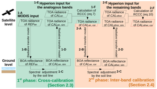
Figure 1.
Schematic diagram of the (1) cross-calibration and (2) inter-band calibration. The input and output data are indicated by black and red parallelograms, respectively. The Moderate Resolution Imaging Spectroradiometer (MODIS) top-of-atmosphere (TOA) radiance (1-A, Section 2.2), the reference for the cross-calibration, was converted into bottom-of-atmosphere (BOA) reflectance via the (1-B) radiative transfer model (RTM). The MODIS BOA reflectance was translated into that of the analogous Hyperion bands via spectral adjustment (1-C) using predetermined soil lines. The simulated BOA reflectance of Hyperion was converted into TOA radiance by the opposite-way RTM (1-D) and compared with the original Hyperion bands (1-E, Section 2.2) to calculate the relative cross-calibration coefficients (RCCCs) for the analogous bands (1-F) based on Equation (7). The first phase output, i.e., calibrated Hyperion bands (2-A) corresponding to MODIS bands, was then used as the reference bands of the second phase. The BOA reflectance of the reference bands was obtained via RTM (2-B) followed by the spectral band adjustment (2-C) to simulate the BOA reflectance of the remaining Hyperion bands. The simulated BOA reflectance was converted into TOA radiance via opposite-way RTM (2-D). By comparing them with the original remaining Hyperion bands (2-E, Section 2.2), the RCCCs (Equation (10)) for the remaining Hyperion bands were obtained (2-F).

Table 1.
Notation conventions.
The following subsections describe the site information (Section 2.1), satellite data for the cross-calibration (Section 2.2), and the detailed procedures of the cross-calibration (Section 2.3) and inter-band calibration (Section 2.4). The implementation of the overall process was performed solely by open-source software (GRASS GIS 7.4.0; QGIS 2.18; Python 3.6.9).
2.1. Site Information
The selected point of interest (38.50486°N, 115.69041°W) was the Railroad Valley Playa (RRVP) desert site, located in central Nevada, U.S. (Figure 2). The MODIS (1 km resolution) and Hyperion (30 m resolution) pixels that included the point were investigated for the calibration (see Section 2.2). The site is frequently used for vicarious and cross-calibration purposes [2,5,29] and is designated as a radiometric calibration network site by the Committee on Earth Observation Satellites [30]. The desert’s spatially homogenous feature helps to mitigate the uncertainty arising from sensor misregistration (even for sensors with a 1–10 km footprint) and discrepancy in sensor geometry, and the dry climate is expected to reduce the influence of atmospheric water vapor and cloud interruption on observations [5,6]. The RRVP site is equipped with stand-alone instruments to measure atmospheric parameters, including the column water vapor and ozone, and the aerosol optical thickness (AOT) at several spectral bands, all of which are available through the Aerosol Robotic Network (AERONET) [31].
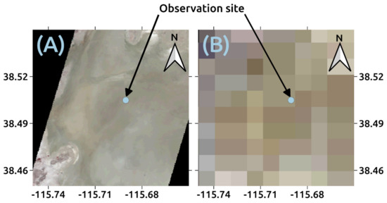
Figure 2.
True-color images of (A) Hyperion and (B) MODIS taken on 2005/08/28 over the Railroad Valley Playa (RRVP) site. The images are shown with geographic projection (latitude–longitude). The blue point indicates the point of interest wherein the in situ field campaigns were conducted.
The National Institute of Advanced Industrial Science and Technology conducted tfield campaigns from 2000 to 2017 (2001/06/14; 2002/06/17; 2003/07/06; 2012/06/28; 2016/06/23; 2017/06/24) to obtain the spectral profile of the soil surface [32], using a FieldSpec spectroradiometer (Malvern Panalytical Ltd., U.K.) and Spectralon standard reflector (Labsphere Inc., U.S.). Because spectral profiles were measured along two different incidence angles, except for 2012/06/28, 11 slightly perturbed soil profiles were obtained.
2.2. Satellite Data for Cross-Calibration
The MODIS daily calibrated radiance L1B (MOD021KM) and corresponding geolocation (MOD03) Collection 6.1 products [33] were downloaded through the Level-1 and Atmosphere Archive & Distribution System Distributed Active Archive Center website [34]. The data were provided with a 1 km spatial resolution and the HDF-EOS format. Although a higher-spatial-resolution product (MOD02HKM) was available, we chose MOD021KM because geometry information is not explicitly included with the former. The HDF-EOS to GeoTIFF conversion tool was used to transform the projection to the same as that of Hyperion (UTM zone 11). The nearest neighbor resampling method was used to conserve the original pixel values. As MODIS is primarily calibrated in reflectance, we converted the original digital number to TOA reflectance multiplied by the cosine of the solar zenith angle, using the provided scaling factor. The derived value was then converted into TOA radiance using the following equation:
where and are the TOA (i.e., at-sensor) radiance [W/(m2 str )] and reflectance, respectively; Esun is the detector-specific weighted solar irradiance [W/(m2 )]; d is the Earth–Sun distance [au]; and is the solar zenith angle [rad]. Esun was provided by the MODIS Characterization Support Team (MCST) [35], and d was found in the HDF files. These data were the references (i.e., REF) and corresponded to 1-A in Figure 1. The calibration uncertainty of Terra MODIS was less than 1.8% in reflectance for visible and near-infrared (VNIR) bands and 1.9–2.6% for shortwave infrared (SWIR) bands because of the crosstalk effect between bands 5 and 7 [25].
Terrain-corrected Hyperion data (L1T) provided by the United States Geological Survey (USGS) Earth Resources Observation and Science Center were downloaded through the EarthExplorer website [36], along with metadata describing the image acquisition time and sensor and solar geometries. Table 2 and Figure 3 show the spectral channels of Hyperion.
Table 2.
Band numbers and corresponding wavelengths of Hyperion. Figure 3 describes the band region for each column with different colors (*1: blue, *2: cyan, *3: green, *4: yellow, *5: orange, and *6: red).
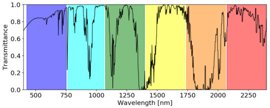
Figure 3.
Hyperion band regions shown in Table 2 and the total transmittance of U.S.-standard atmosphere.
The spatial resolution of Hyperion was 30 m, and the datum/projection was WGS84/UTM at zone 11. Using the USGS-provided scaling factors, the TOA radiance of bands 8–57 for the VNIR domain and 77–224 for the SWIR domain was obtained (the other uncalibrated bands were excluded):
where DN is the digital number for each pixel and the scaling factors are 40 and 80 for the VNIR and SWIR bands, respectively.
These data were to be calibrated, i.e., the analogous bands to MODIS were used as CALan in the cross-calibration (1-E in Figure 1) and the others were used as CALother in the inter-band calibration (2-E in Figure 1). According to previous calibration research [2,5,11,21,22,23,24], the radiometric uncertainty of Hyperion is approximately 5–10% (except for the spectral regions strongly affected by water vapor absorption) and confirmed to be temporally stable during the lifetime.
The cross-calibration uncertainty arising from the geometric discrepancy between sensors is assumed to be limited so long as a homogeneous calibration site is targeted. Furthermore, we selected SNO image pairs to minimize this type of uncertainty. In particular, the pairs were acquired on 18 dates (2001/06/14, 2001/07/16, 2002/06/17, 2002/08/20, 2003/07/22, 2003/10/26, 2003/11/27, 2004/06/06, 2004/06/22, 2004/07/08, 2004/10/12, 2005/08/21, 2005/08/28, 2005/09/29, 2006/11/12, 2007/08/25, 2008/06/01, and 2008/06/24) that ensured (1) a difference in overpass time within 40 min; (2) sensor view angles within 10°; (3) solar incidence angles within 6°; and (4) no cloud contamination, snow cover, or watery ground after heavy rain (checked by visual interpretation). These selection criteria were comparable with those in [8] and were relatively relaxed compared with those in [28]. The criteria were decided because strict criteria reduce not only the cross-calibration uncertainty for one day but also the available number of match-up pairs, particularly since mid-2005, when the orbit of EO-1 changed [11]. After 2011, changing the orbital precession for the mission end [21] substantially altered the temporal coincidence between EO-1 and Terra satellites, so we stopped trying to find pairs.
2.3. Cross-Calibration between Analogous Bands of Hyperion and MODIS
The cross-calibration between analogous bands (Table 3) of Hyperion and MODIS was conducted based on the SNO approach considering the model-based spectral band adjustment and spatial aggregation of Hyperion to match the spatial resolution of MODIS. Although the SNO approach mitigates the uncertainty arising from differences in the geometry and atmospheric conditions between sensors, differences in the RSR and spatial resolution of a pixel remained for this narrow-swath hyperspectral vs. wide-swath multispectral comparison. The difference in the RSR of the analogous bands between sensors (Figure 4) was adjusted based on soil lines, determined by the linear regression between different band-specific soil reflectance. The band-specific reflectance was calculated from the RSR and the soil reflectance profiles obtained multiple ground measurements over the RRVP, as follows:
where is the band k (k = 1, 2,…, 7 for MODIS, and k = 29, 50, 12, 21, 110, 149, or 198 for Hyperion) specific soil reflectance for the sensor m (can be MODIS or Hyperion) derived from , which is the soil reflectance profile along the wavelength () measured by the ith in situ observation (i = 1, 2,…, 11); RSRk,m is the RSR for band k and sensor m. The integration was conducted at the spectral resolution of the in situ observation (1 nm).
Table 3.
Correspondence of the bands between sensors. Each band number and centered wavelength with the full width at half maximum (FWHM) are described.
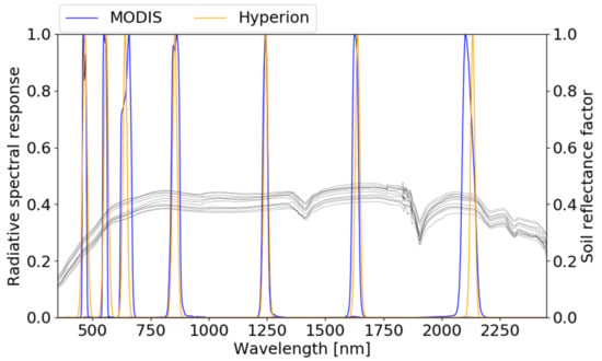
Figure 4.
Relative spectral responses (RSRs) of the analogous bands between sensors. Blue lines: MODIS, orange lines: Hyperion. The black lines are the in situ soil reflectance profiles of the RRVP obtained from the field campaigns (11 times in total).
The RSRs for MODIS were distributed by MCST. However, those for Hyperion could not be found, so they were simulated using a Gaussian function with a full width at half maximum (FWHM) that determined the standard deviation () of the function:
The 11 obtained samples of the band-specific soil reflectance between MODIS and Hyperion were applied to the linear regression via least squares fitting to determine the slope and intercept of each soil line. These parameters were used to translate the BOA reflectance of the MODIS bands into that of the analogous Hyperion bands (1-C in Figure 1).
To make use of the created soil lines, the BOA (i.e., surface) reflectance of each MODIS band at the point of interest was retrieved from the corresponding TOA radiance through the RTM (1-B in Figure 1) via the Second Simulation of a Satellite Signal in the Solar Spectrum—Vector (6SV) version 2.1 code. Since MODIS was the reference sensor (REFan), the original solar irradiance model stored in the 6SV code was altered to that distributed by the MCST, as in [6]. The required atmospheric parameters in 6SV were the column water vapor and ozone amount, AOT at 550 nm, and Junge parameter (i.e., we selected the Junge power-law distribution for the aerosol model). The column water vapor and ozone amount, AOT at 500 nm, and Angstrom parameter near the data acquisition time (within ~40 min) over the RRVP were obtained from AERONET. The AOT at 550 nm was calculated by the following power-law relation:
where AOT550 and AOT500 are the AOT at 550 and 500 nm, respectively, and α is the Angstrom parameter. The Junge parameter γ was approximated by:
and the maximum and minimum radii of the particles were set at 10 and 0.01 micrometers, respectively. Constant values for the real (1.44) and imaginary (0.005) parts of the refractive index were used [37,38].
The simulated surface reflectance of REFan was then translated into Hyperion-like (CALan,sim) surface reflectance using the corresponding soil lines (1-C in Figure 1). Then, the RTM was used along the inverse direction (1-D in Figure 1), with a minor change of the parameter settings regarding the sensor geometry and band response, to retrieve the TOA radiance of CALan,sim. The two-way RTM canceled the errors in the atmospheric parameters to some extent; as a result, the influence of the atmospheric conditions on the calibration result was expected to be limited [7]. We also estimated the uncertainty arising from the atmospheric conditions using the sensitivity analysis (see Appendix A).
Before comparing the TOA radiance of CALan,sim with the original Hyperion radiance, CALan, the Hyperion pixels within a MODIS pixel that included the point of interest were spatially aggregated. The spatial response of the MODIS IFOV [39] was used as the weighting function of the aggregation (Figure 5). Although the area around the point of interest was spatially homogeneous, this process enabled a further reduction in the uncertainty caused by discrepancies in the spatial resolution of the sensors.
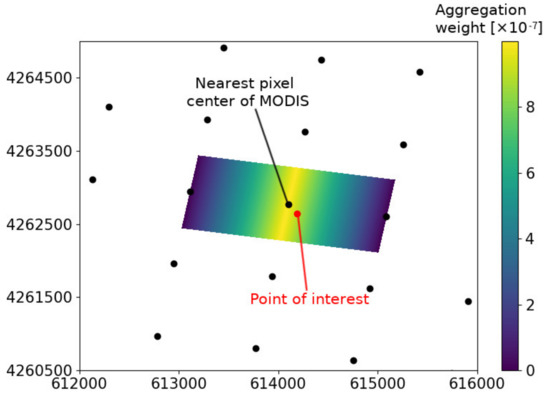
Figure 5.
Weighting function of Hyperion pixels within a MODIS instantaneous field of view (IFOV) on 2005/08/28. The black points indicate the pixel centers of the original MODIS image, and the red point is the point of interest. The x-y axes are the meter coordinates on the UTM (zone 11) projection.
By comparing CALan with CALan,sim, the RCCC (1-F in Figure 1) was defined by:
where Ik,CALan,sim and Ik,CALan are the band k TOA radiance of CALan,sim and spatially aggregated CALan, respectively, and RCCCk is the band k RCCC. Although [28] defined the RCCC in the reflectance domain, the radiance based RCCC was defined here because Hyperion was calibrated in the radiance domain.
To evaluate the consistency between Hyperion and MODIS, the relative mean bias () and the root-mean-square relative error (RMSEk) for each band k in unit of percent were calculated:
where i is the index of data acquisition days and N is the total number of data acquisition days (N = 18). The interpretation of the other variables was the same as in Equation (7).
2.4. Inter-Band Calibration of Hyperion
The corrected Hyperion bands (CALan,cor) from the previous phase were used as the reference bands in the inter-band calibration phase (2-A in Figure 1). This phase included similar procedures as the previous ones, i.e., a two-way RTM and band translation based on the soil lines. The major difference was that a large combination of bands (the seven reference bands multiplied by the other 191 bands, i.e., 1,337) had to be considered in the determination of the soil lines, and multiple bands (at most, seven analogous bands) could be used as the reference.
The selection of the reference bands seemed to introduce major uncertainty in the calibration results. Increasing the reference bands (and taking their average for the resultant RCCC) did not necessarily improve the calibration accuracy because the linear relationship was blurred when comparing spectrally far bands (Figure 6). Therefore, we selected the two spectrally closest analogous bands to the band to be calibrated (i.e., CALother) and used the average of the results to calculate the RCCC. For Hyperion bands beyond the range of the Hyperion analogous bands (i.e., bands 8–11 and 199–224), only the nearest reference band (i.e., band 12 or 198) was used.
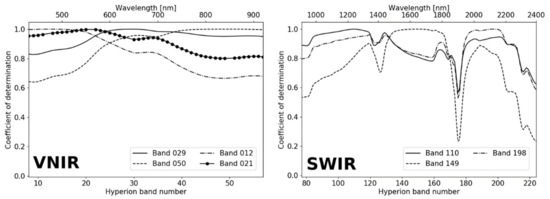
Figure 6.
Coefficient of determination (R2) for each Hyperion analogous band to MODIS for (left) visible and near-infrared (VNIR) bands and (right) shortwave infrared (SWIR) bands. At neighboring bands, R2 tended to show the highest value. Near water vapor absorption regions in SWIR, R2 substantially dropped.
The remaining process was similar to the previous phase: the reference band (CALan,cor) was converted into surface reflectance by the RTM (2-B in Figure 1), followed by band translation using the soil lines (2-C in Figure 1) and opposite-way RTM (2-D in Figure 1) to obtain the TOA radiance of CALother,sim. The RCCC for CALother (2-F in Figure 1) was defined by:
where Ik,CALother,sim and Ik,CALother are the band k TOA radiance of CALother,sim and CALother, respectively. No spatial aggregation was conducted in this phase because there was no discrepancy in the spatial resolution between CAL and REF.
3. Results
3.1. Cross-Calibration between the Analogous Bands of Hyperion and MODIS
Table 4 lists the relative mean bias () and RMSEk. The VNIR bands showed less in absolute value (approximately 3–5%) and less RMSEk (approximately 4–6%) than the SWIR bands (approximately 7–9% for both the absolute and RMSEk). The largest RMSEk in the VNIR region was found in the blue band (MODIS band 3) because of the underestimation of the TOA radiance by Hyperion, which also slightly overestimated the TOA radiance in the other three bands (green, red, and NIR). In the SWIR region, the TOA radiance in shorter-wavelength bands (MODIS bands 5 and 6) was underestimated, whereas that in the rest was overestimated. Among all the analogous bands of Hyperion, the shorter-wavelength SWIR (MODIS band 5 or Hyperion band 110) was the most biased, requiring substantial correction by the smallest RCCC. The RCCCs ranged approximately from 0.92 to 1.07, with 0.021–0.025 standard deviation. It could also be expressed as 2.2–2.7% standard deviation, comparable with McCorkel et al.’s [22] reported 2% standard deviation of vicarious calibration.
Table 4.
Radiometric consistency and RCCC between MODIS and Hyperion. The bottom row shows the temporal average of the RCCC with standard deviation.
Such characteristics were also confirmed in Figure 7, which compares the TOA radiance between CALan and CALan,sim. Less Hyperion radiance was observed in the blue and two of the shorter-wavelength SWIR bands, causing less slope in the linear regression than unity. Only one SWIR band showed larger slope than unity, reflecting the overestimation tendency of TOA radiance in Hyperion band 198 (Table 4). Every analogous band showed strong linearity (over 0.98 in R2).
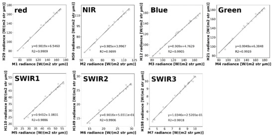
Figure 7.
Scatterplot of the TOA radiance between the MODIS and Hyperion analogous bands in red, NIR, blue, green, and SWIR bands.
The time series variation of the RCCC is shown in Figure 8. The variation range was approximately ±0.02 in RCCC, which was approximately consistent with the standard deviation results shown above. Slightly increasing temporal trends (i.e., a positive slope in the regression lines) were observed in most bands, some of which (Hyperion bands 21, 29, and 50) were statistically significant (p < 0.05). In contrast, the longest wavelength band (Hyperion band 198) showed no increasing tendency. This could be partially attributed to the relatively low solar radiation energy blurring meaningful signals over noise in the longest wavelength region rather than the inherent sensor feature.
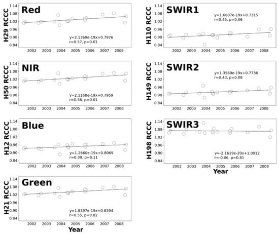
Figure 8.
Time series of the RCCC for each Hyperion analogous band to MODIS. The red, NIR, blue, green, and SWIR bands correspond to MODIS bands 1–7 and Hyperion bands 29, 50, 12, 21, 110, 149, and 198, respectively. The linear regression line was drawn, and its mathematical expression with the correlation coefficient (r) and p-value was described over the plots. The explanatory variable (x) in the linear regression is the Unix time of the data acquisition.
3.2. Inter-Band Calibration of Hyperion
Figure 9 compares the TOA radiance of CALother and CALother,sim simulated from each reference band using four typical days as examples. To some extent, a similar tendency as the previous cross-calibration results was observed: a slight overestimation in visible bands, except the blue band, and relatively large underestimation in the shorter-wavelength SWIR region. However, there was nonnegligible band-to-band variation, causing several different characteristics from those shown in the cross-calibration: overestimation in the shortest-wavelength visible spectral region, slight underestimation over the continuous NIR region, and almost identical TOA radiance in the longer-wavelength SWIR region. The original TOA radiance in the wavebands was much less than that in the simulated radiance, arguably because of atmospheric gas absorption (ca. oxygen at 760 nm, carbon dioxide at 2000 nm, and water vapor at 940 nm, 1140 nm, and regions masked by gray rectangles in Figure 9). Interestingly, the band-to-band variation patterns were similar from day to day, suggesting an inherent feature of each band. Since the solar elevation angle was low in autumn (2003/11/27), the absolute value of the TOA radiance was small (Figure 9B,F).
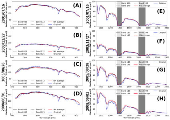
Figure 9.
Comparison of the TOA radiance between CALother and CALother,sim. The black lines are the CALother,sim TOA radiance simulated from each reference band, the red line is the averaged value of the nearest neighbor CALother,sim (see Section 2.4), and the blue line is the original Hyperion TOA radiance to be calibrated (CALother). (A–D) are the results for the VNIR region on the day indicated along the left axis, and (E–H) are those for the SWIR region. The gray masks show uncertain spectral regions due to strong water vapor absorption.
The difference among the TOA radiance simulations originating from different reference bands was generally small, except in the shortest-wavelength visible (blue) spectral region and several SWIR regions (black lines in Figure 9). This discrepancy became apparent when looking at the RCCCs along the wavelength (Figure 10). The Hyperion calibration is good enough soon after the launch (2001/07/16), except for the spectral edge and water absorption bands. After 2003, the band-to-band variation from unity increased. The temporal variation range was estimated by the temporal standard deviation in the RCCCs (dashed lines in Figure 10E,J). Similar to the cross-calibration result, the standard deviation of the RCCCs ranged from 0.02 to 0.03 in almost all VNIR bands (except the NIR edge region: ~0.04). The standard deviation in the SWIR region was typically less than 0.04, except for the water absorption bands and SWIR edge region (from Hyperion band 213 onward), probably because of the limitation of the sensor’s signal-to-noise ratio.
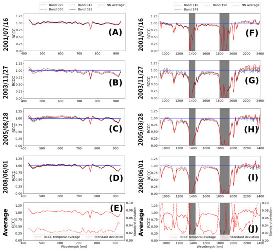
Figure 10.
RCCCs of CALother with reference to CALother,sim. (A–D) are the results for the VNIR region on the day indicated along the left axis, and (F–I) are the results for the SWIR region. The black lines are the RCCCs simulated from each reference band, the red solid line is the averaged value of the nearest neighbor CALother,sim (see Section 2.4), and the blue line shows the unity (i.e., the ideal quality in CALother). (E,I) describe the 18-day temporal average (solid lines) of the RCCCs and their temporal standard deviations (dashed lines) for the VNIR and SWIR regions, respectively. The gray masks show uncertain spectral regions due to strong water vapor absorption.
The mitigation of the band-to-band variation was also evaluated by checking the continuity of the TOA radiance within a narrow spectral region. Specifically, we applied linear regression to TOA radiances from several adjacent bands of Hyperion within 620–670, 841–876, 459–479, 545–565, 1230–1250, 1628–1652, and 2105–2155 nm (corresponding to the MODIS band regions) separately to remove the linear trend from the data within the narrow region. We then calculated the standard deviation of the trend-removed data and averaged it over the four example days in Figure 9 and Figure 10. Table 5 shows the result, revealing that the band-to-band variation was substantially mitigated for all regions corresponding to MODIS bands. Evaluating the spectrally smooth pattern in TOA radiance (Figure 9), the band-to-band variation in the other spectral regions is also likely to be mitigated.
Table 5.
Comparison of the band-to-band variation between the TOA radiance of the original Hyperion and that after our calibration. The standard deviation in the radiance unit [W/(m2 str )] was averaged over four days (2001/07/16, 2003/11/27, 2005/08/28, and 2008/06/01).
The time series patterns of the spectral RCCCs are shown as a heatmap (Figure 11). Obviously low RCCCs were observed near the water absorption bands. An apparently increasing temporal trend in a number of visible bands and several NIR bands was also observed, similar to the cross-calibration results. In contrast, few bands showed any significant temporal trend in the SWIR regions, except for the water absorption bands. These different temporal trends among the bands seemed to exaggerate the band-to-band variation over time, as partly shown in Figure 10. Consistent with the results in Section 3.1, the TOA radiance in the visible bands and longer-wavelength SWIR bands tended to be positively biased (RCCC > 1.0), whereas that in the shorter-wavelength SWIR bands tended to be negatively biased (RCCC < 1.0). Scatterplots and time series similar to those for cross-calibration were shown as examples in Figure 12 and Figure 13, for Hyperion bands with 200 nm steps within the range of MODIS analogous bands (500, 700, 900, 1100, 1300, 1500, 1700, and 2100 nm). The strong water absorption band (1900 nm) was excluded. In comparison to the cross-calibration results, less slope in the linear regression than unity and blurred linearity tended to be observed in the scatterplot (Figure 12) on the bands being slightly affected by atmospheric absorption (900, 1100, 1300, and 1500 nm). Other than those bands, good consistency between the original and the simulated Hyperion radiance was confirmed. In time series (Figure 13), a significant increasing trend at 500 nm was observed, confirming the tendency found in the heatmap (Figure 11).
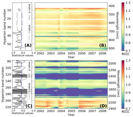
Figure 11.
Heatmap of the time series RCCCs for each Hyperion band (B,D) and the statistical significance in their temporal trends (A,C). (A,B) are for the VNIR bands, and (C,D) are for the SWIR bands. In (A,C), the correlation coefficient (r) and p-value of the linear regression of the RCCCs over time are shown. The blue line is the statistical significance level of the p-value (p < 0.05). Strong water absorption bands are masked by the gray rectangle in the SWIR region. In (B,D), the analogous bands used in the previous cross-calibration (Hyperion bands 12, 21, 29, 50, 110, 149, and 198) were excluded from the plot. The spline function interpolated the gaps between the image acquisitions.
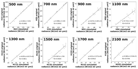
Figure 12.
Scatterplot of the TOA radiance between the simulated and the original Hyperion bands at wavelengths 500, 700, 900, 1100, 1300, 1500, 1700, and 2100 nm.
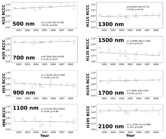
Figure 13.
Time series of the RCCC for Hyperion bands at wavelengths 500, 700, 900, 1100, 1300, 1500, 1700, and 2100 nm. The linear regression line was drawn, and its mathematical expression with the correlation coefficient (r) and p-value was described over the plots. The explanatory variable (x) in the linear regression is the Unix time of the data acquisition.
4. Discussion
The doubled use of the model-based spectral band adjustment approach provided simultaneous correction of the inter-sensor and intra-sensor (i.e., inter-band) biases of the hyperspectral sensor. The improvement of the inter-sensor consistency (correction of the bias shown in Table 4) could contribute to improving the accuracy of continuous Earth observation using multiple sensors [5,6,11,14,15], as well as spatiotemporal sensor fusion applications [40,41,42], that enable the creation of long-term, high-spatiotemporal-resolution datasets [43,44]. Since this is cross-calibration, unlike vicarious calibration such as a reflectance-based approach, the collection of the ground reflectance data that is temporally and geometrically coincident with the view of the site by the sensor [11] is not required.
Furthermore, an improvement in the inter-band consistency is the other important aspect of our work. Mitigating substantial (5–10%) band-to-band variation in Hyperion [11,22] could aid satellite-based monitoring in the fields of ecology [2], agriculture [3], and geology [4], which makes full use of the narrow-band nature of hyperspectral sensors. The quality-assured hyperspectral dataset also provides opportunities for a more accurate spectral band adjustment using spaceborne hyperspectral data (e.g., [10]).
The cross-comparison between analogous Hyperion and MODIS bands considering spectral band adjustment and spatial aggregation showed approximately 4–6% and 7–9% of the RMSEk in the TOA radiance [W/(m2 str )] at the VNIR and SWIR regions, respectively. The agreement levels were consistent with the previous cross-comparison research between Hyperion and MODIS [5,11], thus supporting the validity of our approach. The correction coefficient of the sensor bias, RCCC, ranged approximately from 0.92 to 1.07 with a standard deviation of 2.2–2.7% among all analogous Hyperion to MODIS bands.
The inter-band calibration provided RCCCs for all the spectral bands of Hyperion. The RCCCs typically ranged from 0.9 to 1.1 (i.e., within 10%-level biases), except for the water absorption bands, with a 0.02–0.03 temporal standard deviation in almost all VNIR bands (except the NIR edge region) and, typically, less than 0.04 temporal standard deviation in the SWIR region (except for the water absorption bands and spectral edge region, from Hyperion band 213 onward). The comparable or slightly larger standard deviation in the RCCCs for the remaining bands (0.02–0.03 in VNIR and <0.04 in SWIR; Figure 10) other than the analogous bands (0.021–0.025 in all regions; Table 4) that were directly derived from the reference sensor (MODIS) implied an accumulation of the uncertainty in the first (cross-calibration) and second phases (inter-band calibration). Based on the sensitivity analysis [6,19,45] and literature reviews about the solar irradiance model [46,47], uncertainty for each phase (CALan,sim and CALother,sim) was estimated in Table 6 and Table 7 (see Appendix A for detail). The uncertainty in the first phase’s results (CALan,cor;; 2.5–3.2% in the root sum of squares) was taken over in the second phase, resulting in the uncertainty in CALother,sim, which was identical to the uncertainty in the resultant calibrated radiance in the remaining Hyperion bands (CALother,cor). For all investigated bands, the overall uncertainty was within the radiometric accuracy in the original Hyperion (approximately 5–10% [2,5,11,21,22,23,24]); however, it ranges depending on the band from 2.5% to 4.8% in the root sum squares (Table 7). A substantial part of this variability can be explained by the impact of atmospheric condition variability on the bands being slightly affected by atmospheric absorption (900, 1100, and 1500 nm) in the inter-band calibration. This may relate to the blurred linearity in the scatterplot (Figure 12) and inconstant RCCCs in time series (Figure 13) on such bands. In contrast, atmospheric condition variability has a limited effect on cross-calibration, probably because of the canceled bias along the two-way radiative transfer simulation [7]. We could also confirm that the effect of the geolocation error was limited over RRVP because of the spatial homogeneity. Across all bands, uncertainties in the MODIS reflectance and solar irradiance model were predominant, whereas the soil line had secondary effects. Future research should consider such uncertainty features for the reference band selection in inter-band calibration. For the soil line, the RSR interpolation procedure and spectral resolution setting in the integration (Equation (3)) may also affect the uncertainty. Since the in situ soil spectra were mainly acquired in June and July, uncertainty in the soil line for the inter-band calibration in the other season is possibly large. This may be an explanation for the relatively good consistency among the results using different reference bands in June and July (black lines in Figure 9A,D and Figure 10A,D).
Table 6.
Error budget table for the cross-calibrated Hyperion bands. Each column shows relative uncertainty [%] in each MODIS analogous band (from MODIS bands 1 to 7). The estimation process was described in the Appendix A.
Table 7.
Error budget table for inter-band-calibrated Hyperion (CALother,sim). Relative uncertainty estimation [%] for eight band cases were shown as examples. The uncertainty in the cross-calibrated radiance of the Hyperion reference bands was considered from the results in Table 6 (combined uncertainty was calculated from those of the two nearest bands).
The band-to-band variation pattern became inherent over time (Figure 9 and Figure 10), roughly characterized by positive bias of Hyperion’s radiance at the spectral edge of the blue band, negative bias approximately 450 nm, slightly positive bias in most of the VNIR region (500–700 nm), negative bias in the NIR region (700–950 nm), and relatively large negative bias in the broad SWIR region (950–1,200 nm and 1,500–1,800 nm), except for the atmospheric absorption region and SWIR spectral edge. The observed pattern was consistent with the previous cross-comparison research on MODIS and Hyperion (Figure 5 in [11]).
However, the deviation from unity seemed to gradually exaggerate after the sensor launch, creating increasing temporal trends in the RCCCs for several bands (particularly in the visible region) during 2001–2008 (Figure 8 and Figure 11). This result was not consistent with that of the existing research [2,11,21,22,24], which has reported that Hyperion radiance data are temporally stable or even decreasing for some bands over their lifetime. One possible interpretation for this discrepancy is that the RCCCs may have been affected by the orbit change after 2005, making it difficult to find highly consistent (i.e., less differences in the acquisition time and sensor or solar angles) SNO pairs [11]. The relatively inconsistent pairs biased the recent RCCCs in the time series, resulting in the artificial increasing trends. As the outliers in Figure 8 tended to be found in the autumn (2003/10/26, 2003/11/27, 2006/11/12), a season with low solar elevation angles may also lead to an unreliable RCCC estimation. Moreover, uncertainty in the reference sensor (MODIS) [25] also affected the RCCC estimation.
Therefore, this apparent temporal trend obtained from the limited number of samples does not necessarily demonstrate the sensor degradation trend of Hyperion. Further investigation with a larger sample size is required to reveal this feature of the Hyperion dataset, particularly after 2005. Revealing the dataset’s spectral and temporal behavior in detail, especially for its analogous bands to MODIS, will help with the selection of the reference bands in inter-band calibration. The use of non-coincident pairs with similar geometry [11] or in consideration of BRDF [17,24] as well as the use of other multispectral satellites, including geostationary satellites, as references [13] could increase the sample size. Using other RadCalNet sites [30] or pseudo-invariant calibration sites [48] also helps to increase calibration opportunities. Such an attempt would also aid cross-calibration for sensors aboard the International Space Station that have irregular overpass times at specific calibration sites, such as the German Aerospace Center Earth Sensing Imaging Spectrometer (DESIS) [49] and Hyperspectral Imager SUIte (HISUI) [50]. Potentially, the first (cross-calibration) and second (inter-band calibration) steps of our approach are separately applicable. This feature could provide flexible calibration for future hyperspectral satellites. For example, we could conduct cross-calibration with coincident pairs of hyperspectral data and other available reference data over a suitable target first and, then, conduct inter-band calibration for all available hyperspectral data (including unpaired data with reference data) over the other calibration sites independently.
Overall, to improve inter-sensor consistency with MODIS and inter-band consistency within Hyperion, the provided RCCCs during 2001–2008 were useful, keeping the 0.02–0.03 VNIR and 0.04 SWIR temporal standard deviations in mind. Note that the RCCCs were highly uncertain near atmospheric absorption bands (Figure 10), both the wide water absorption bands [2] and the relatively narrow bands (e.g., oxygen at 760 nm, carbon dioxide at 2000 nm, and water vapor at 940 and 1140 nm [51]), as demonstrated by the low RCCC areas in the heatmap (Figure 11). The spectral edge region, particularly in NIR and SWIR, also showed high uncertainty (Figure 10). In the estimated error budget (Table 6 and Table 7), the uncertainty in the solar irradiance model was the second largest source of error [6,7,19] after the calibration uncertainty in the reference data (except atmospheric absorption regions). We used the solar irradiance model distributed by MCST considering the consistency with retrieved ancillary parameters in the reference sensor (MODIS) such as Esun. However, the uncertainty estimation in our approach arising from the selection of the solar irradiance model should be addressed in the future. The influence from the discrepancy in the geometry and atmospheric conditions between data acquisitions was limited as long as we used SNO pairs over a homogeneous calibration site with a two-way RTM, but it should be considered when using non-coincident or different-geometry pairs through investigating the effect of variation of acquisition time, and sensor and solar angles on RCCC estimation. Inter-comparison between various calibration approaches and our approach will also help to reveal the detailed potential and limitations of our approach, including checking whether the time series feature of Hyperion (Figure 8 and Figure 11) is observed by other approaches under the same study condition.
5. Conclusions
This study proposed an operational approach for the simultaneous correction of inter-sensor and intra-sensor (i.e., inter-band) biases in hyperspectral sensors, using EO-1 Hyperion and Terra MODIS as examples. The approach includes the double use of a model-based spectral band adjustment, which fully utilizes the soil line concept. The cross-comparison results over the RRVP calibration site showed that the discrepancy in the analogous bands between Hyperion and MODIS during 2001–2008 was approximately 4–6% and 7–9% of the RMSE in the TOA radiance at the VNIR and SWIR regions, respectively. For all bands, except the uncalibrated bands of Hyperion, the RCCCs were derived from the coincident Hyperion and MODIS pairs during 2001–2008. The RCCCs typically ranged from 0.9 to 1.1, with a standard deviation of 0.02–0.03 for VNIR and 0.04 for SWIR, except for the strong water absorption bands. The application of the proposed approach consolidated with non-coincident or different-geometry image pairs using BRDF correction as well as with other multispectral sensors, including geostationary satellite sensors, as references is a promising avenue to providing more flexible cross-calibration for irregular-orbit sensors aboard the International Space Station.
Author Contributions
H.M. established the basic research design, implemented the algorithm, conducted all analyses including software preparation, satellite data collection (MODIS and Hyperion), validation and visualization, and wrote the manuscript. K.O. developed the original concept of model-based spectral band adjustment. S.T., K.O., H.Y., conducted the field survey. H.M., S.T., K.O., H.Y., and S.Y. have contributed to the detailed research design and interpretation of the results, edited the manuscript, read, and agreed to the published version of the manuscript.
Funding
This research was funded by the Ministry of Economy, Trade and Industry of Japan (METI; no grant number).
Acknowledgments
The present study was supported by METI. The authors appreciate members of the Hyperspectral Imager SUIte (HISUI) calibration working group.
Conflicts of Interest
The authors declare no conflict of interest.
Appendix A
The uncertainties of cross-calibration and inter-band calibration were evaluated based on sensitivity analysis [6,19,45] and literature reviews [25,46,47]. For cross-calibration, we considered the impact of:
- (1)
- radiometric calibration uncertainty of MODIS,
- (2)
- variability in atmospheric conditions,
- (3)
- soil line influence,
- (4)
- geolocation error of Hyperion, and
- (5)
- solar irradiance model
on each MODIS analogous band of Hyperion. (1) The uncertainty of the MODIS reflectance was estimated in previous research [25] for each solar reflective band.
(2) Atmospheric conditions were evaluated by the sensitivity analysis. First, TOA radiances of MODIS and Hyperion were retrieved from temporally averaged in situ soil reflectance using the 6SV 2.1 code with temporally averaged atmospheric conditions over 18 observation days (Table A1). Then we conducted a two-way radiative transfer simulation using the 6SV code and band adjustment with atmospheric parameter sets perturbed around the averaged value, to translate the MODIS TOA radiance into Hyperion-like TOA radiance. In particular, three cases (mean minus standard deviation, mean, and mean plus standard deviation) for each parameter (AOT at 550 nm, the Junge parameter, the column water vapor, column ozone amount) were input in 6SV. The imaginary part of the refractive index also ranged in 0.001, 0.005, and 0.01. The perturbed output of the Hyperion-like TOA radiance was then compared with the original Hyperion TOA radiance obtained under the averaged atmospheric condition, calculating the relative bias (%) of them. We used the standard deviation of the relative bias to estimate the uncertainty arising from atmospheric conditions.
Table A1.
Mean and standard deviation of the atmospheric conditions among the observation images.
Table A1.
Mean and standard deviation of the atmospheric conditions among the observation images.
| AOT at 550 nm | Junge Parameter | Water Vapor (g/cm2) | Ozone (Dobson Unit) | |
|---|---|---|---|---|
| Mean | 0.074 | 3.25 | 0.81 | 296.3 |
| Standard deviation | 0.053 | 0.49 | 0.40 | 17.1 |
Uncertainty arising from (3) in situ soil spectrum was estimated as follows: 11 samples of BOA reflectance of MODIS were calculated from the in situ soil spectrum and translated into Hyperion-like BOA reflectance using the soil line. The Hyperion-like BOA reflectance was translated into Hyperion-like TOA radiance using the 6SV 2.1 code with an averaged atmospheric condition, which was compared with the original Hyperion TOA radiance. The standard deviation of the relative bias was used to estimate uncertainty of this factor.
Uncertainty arising from (4) geolocation error of Hyperion was estimated by conducting spatial aggregation with slightly shifted real Hyperion images [6,45]. According to [52], the MODIS absolute geolocation error was reported as <45 m. For the Hyperion L1T product, the terrestrial correction was based on shuttle radar topography mission data, with an absolute geolocation error of 12. 6 m [53]. Given those estimations, we assumed that the relative geolocation error was <60 m (two pixels of Hyperion). The real Hyperion images were shifted −2, 0, or +2 pixels along the x and/or y directions in the UTM projection, obtaining eight direction-shifted images for each day. Spatial aggregation within MODIS IFOV was conducted for the shifted images, and an absolute value of the relative difference between the original image (without shift) and the shifted image was calculated. The absolute values were averaged for all direction and observation days. The averaged value was the estimation of uncertainty arising from the geolocation error.
A more detailed background and the procedure of the sensitivity analyses were described in [6]. The last evaluated factor for the cross-calibration was uncertainty in the solar irradiance model. The MCST solar irradiance model is a combination of the data from Thuillier et al. [46] and Neckel and Labs [54]. The uncertainty of the model has been reported in [46,47], which were used to estimate uncertainty in the solar irradiance data for each analogous band of Hyperion.
For inter-band calibration, we evaluated the impact of:
- (1)
- the Hyperion reference bands,
- (2)
- variability in atmospheric conditions,
- (3)
- soil line influence, and
- (4)
- solar irradiance model
for several Hyperion calibration bands with 200 nm steps within the range of MODIS analogous bands (500, 700, 900, 1100, 1300, 1500, 1700, and 2100 nm) as examples. The strong water absorption band (1900 nm) was excluded from this evaluation. (1) Uncertainty in the Hyperion reference bands was estimated above. Note that we used the average of the two neighboring reference bands for the inter-band calibration. When we assume that the uncertainties in the two references are independent of each other, the combined uncertainty (sum) in the averaged result from the first reference (with uncertainty 1) and the second reference (with uncertainty 2) can be written as:
References
- Transon, J.; d’Andrimont, R.; Maugnard, A.; Defourny, P. Survey of hyperspectral earth observation applications from space in the Sentinel-2 context. Remote Sens. 2018, 10, 157. [Google Scholar] [CrossRef]
- Campbell, P.K.E.; Middleton, E.M.; Thome, K.J.; Kokaly, R.F.; Huemmrich, K.F.; Lagomasino, D.; Novick, K.A.; Brunsell, N.A. EO-1 Hyperion reflectance time series at calibration and validation sites: Stability and sensitivity to seasonal dynamics. IEEE J-STARS 2013, 6, 276–290. [Google Scholar] [CrossRef]
- Marshall, M.; Thenkabail, P. Advantage of hyperspectral EO-1 Hyperion over multispectral IKONOS, GeoEye-1, WorldView-2, Landsat ETM+, and MODIS vegetation indices in crop biomass estimation. ISPRS J. Photogramm. 2015, 108, 205–218. [Google Scholar] [CrossRef]
- Van der Meer, F.D.; van der Werff, H.M.A.; van Ruitenbeek, F.J.A.; Hecker, C.A.; Bakker, W.H.; Noomen, M.F.; van der Meijde, M.; Carranza, E.J.M.; de Smeth, J.B.; Woldai, T. Multi- and hyperspectral geologic remote sensing: A review. Int. J. Appl. Earth Obs. 2012, 14, 112–128. [Google Scholar] [CrossRef]
- Thome, K.J.; Biggar, S.F.; Wisniewski, W. Cross comparison of EO-1 Sensors and other earth resources sensors to Landsat-7 ETM+ using Railroad Valley Playa. IEEE Trans. Geosci. Remote Sens. 2003, 41, 1180–1188. [Google Scholar] [CrossRef]
- Obata, K.; Tsuchida, S.; Yamamoto, H.; Thome, K. Cross-calibration between ASTER and MODIS visible to near-infrared bands for improvement of ASTER radiometric calibration. Sensors 2017, 17, 1793. [Google Scholar] [CrossRef]
- Obata, K. Sensitivity analysis method for spectral band adjustment between hyperspectral sensors: A case study using the CLARREO Pathfinder and HISUI. Remote Sens. 2019, 11, 1367. [Google Scholar] [CrossRef]
- Heidinger, A.K.; Cao, C.; Sullivan, J.T. Using Moderate Resolution Imaging Spectrometer (MODIS) to calibrate advanced very high resolution radiometer reflectance channels. J. Geophys. Res. Atmos. 2002, 107. [Google Scholar] [CrossRef]
- Wu, A.; Xiong, X.; Cao, C. Terra and Aqua MODIS inter-comparison of three reflective solar bands using AVHRR onboard the NOAA-KLM satellites. Int. J. Remote Sens. 2008, 29, 1997–2010. [Google Scholar] [CrossRef]
- Barrientos, C.; Mattar, C.; Nakos, T.; Perez, W. Radiometric cross-calibration of the Chilean satellite FASat-C using RapidEye and EO-1 Hyperion data and a simultaneous nadir overpass approach. Remote Sens. 2016, 8, 612. [Google Scholar] [CrossRef]
- McCorkel, J.; Thome, K.; Lockwood, R.B. Absolute radiometric calibration of narrow-swath imaging sensors with reference to non-coincident wide-swath sensors. IEEE Trans. Geosci. Remote Sens. 2013, 51, 1309–1318. [Google Scholar] [CrossRef]
- Mishra, N.; Haque, M.O.; Leigh, L.; Aaron, D.; Helder, D.; Markham, B. Radiometric cross calibration of Landsat 8 Operational Land Imager (OLI) and Landsat 7 Enhanced Thematic Mapper Plus (ETM+). Remote Sens. 2014, 6, 12619–12638. [Google Scholar] [CrossRef]
- Yu, F.; Wu, X. Radiometric inter-calibration between Himawari-8 AHI and S-NPP VIIRS for the solar reflective bands. Remote Sens. 2016, 8, 165. [Google Scholar] [CrossRef]
- Teillet, P.M.; Fedosejevs, G.; Thome, K.J.; Barker, J.L. Impacts of spectral band difference effects on radiometric cross-calibration between satellite sensors in the solar-reflective spectral domain. Remote Sens. Environ. 2007, 110, 393–409. [Google Scholar] [CrossRef]
- Chander, G.; Mishra, N.; Helder, D.L.; Aaron, D.B.; Angal, A.; Choi, T.; Xiong, X.; Doelling, D.R. Applications of spectral band adjustment factors (SBAF) for cross-calibration. IEEE Trans. Geosci. Remote Sens. 2013, 51, 1267–1281. [Google Scholar] [CrossRef]
- Yuan, K.; Thome, K.; McCorkel, J. Radiometric cross-calibration of Terra ASTER and MODIS. In Proceedings of the SPIE Optical Engineering + Applications, San Diego, CA, USA, 9–13 August 2015; Volume 9607, p. 960724. [Google Scholar]
- Farhad, M.M.; Kaewmanee, M.; Leigh, L.; Helder, D. Radiometric cross calibration and validation using 4 angle BRDF model between Landsat 8 and Sentinel 2A. Remote Sens. 2020, 12, 806. [Google Scholar] [CrossRef]
- Baret, F.; Jacquemoud, S.; Hanocq, J.F. About the soil line concept in remote sensing. Adv. Space Res. 1993, 13, 281–284. [Google Scholar] [CrossRef]
- Obata, K.; Tsuchida, S.; Iwao, K. Inter-band radiometric comparison and calibration of ASTER visible and near-infrared bands. Remote Sens. 2015, 7, 15140–15160. [Google Scholar] [CrossRef]
- Ungar, S.G.; Pearlman, J.S.; Mendenhall, J.A.; Reuter, D. Overview of the earth observing one (EO-1) mission. IEEE Trans. Geosci. Remote Sens. 2003, 41, 1149–1159. [Google Scholar] [CrossRef]
- Franks, S.; Neigh, C.S.R.; Campbell, P.K.; Sun, G.; Yao, T.; Zhang, Q.; Huemmrich, K.F.; Middleton, E.M.; Ungar, S.G.; Frye, S.W. EO-1 data quality and sensor stability with changing orbital precession at the end of a 16 year mission. Remote Sens. 2017, 9, 412. [Google Scholar] [CrossRef]
- McCorkel, J.; Thome, K.; Ong, L. Vicarious calibration of EO-1 hyperion. IEEE J-STARS 2013, 6, 400–407. [Google Scholar] [CrossRef]
- Czapla-Myers, J.; Ong, L.; Thome, K.; McCorkel, J. Validation of EO-1 hyperion and advanced land imager using the radiometric calibration test site at railroad valley, Nevada. IEEE J-STARS 2016, 9, 816–826. [Google Scholar] [CrossRef]
- Jing, X.; Leigh, L.; Helder, D.; Pinto, C.T.; Aaron, D. Lifetime absolute calibration of the EO-1 Hyperion sensor and its validation. IEEE Trans. Geosci. Remote Sens. 2019, 57, 9466–9475. [Google Scholar] [CrossRef]
- Xiong, X.; Sun, J.; Wu, A.; Chiang, K.-F.; Esposito, J.; Barnes, W. Terra and Aqua MODIS calibration algorithms and uncertainty analysis. In Proceedings of the SPIE Remote Sensing, Bruges, Belgium, 19–22 September 2005; Volume 5978, p. 59780V. [Google Scholar]
- Yokoya, N.; Mayumi, N.; Iwasaki, A. Cross-calibration for data fusion of EO-1/Hyperion and Terra/ASTER. IEEE J-STARS 2013, 6, 419–426. [Google Scholar] [CrossRef]
- Ravi Shankar, D. Remote Sensing of Soils: Earth Observation Systems; Springer: Berlin/Heidelberg, Germany, 2017; p. 70. [Google Scholar]
- Lacherade, S.; Fougnie, B.; Henry, P.; Gamet, P. Cross calibration over desert sites: Description, methodology, and operational implementation. IEEE Trans. Geosci. Remote Sens. 2013, 51, 1098–1113. [Google Scholar] [CrossRef]
- Scott, K.P.; Thome, K.J.; Brownlee, M.R. Evaluation of the Railroad Valley Playa for use in vicarious calibration. In Proceedings of the SPIE’s 1996 International Symposium on Optical Science, Engineering, and Instrumentation, Denver, CO, USA, 4–9 August 1996; Volume 2818, pp. 158–166. [Google Scholar]
- Bouvet, M.; Thome, K.; Berthelot, B.; Bialek, A.; Czapla-Myers, J.; Fox, N.P.; Goryl, P.; Henry, P.; Ma, L.; Marcq, S.; et al. RadCalNet: A radiometric calibration network for Earth observing imagers operating in the visible to shortwave infrared spectral range. Remote Sens. 2019, 11, 2401. [Google Scholar] [CrossRef]
- Giles, D.M.; Sinyuk, A.; Sorokin, M.G.; Schafer, J.S.; Smirnov, A.; Slutsker, I.; Eck, T.F.; Holben, B.N.; Lewis, J.R.; Campbell, J.R.; et al. Advancements in the Aerosol Robotic Network (AERONET) Version 3 database—Automated near-real-time quality control algorithm with improved cloud screening for Sun photometer aerosol optical depth (AOD) measurements. Atmos. Meas. Tech. 2019, 12, 169–209. [Google Scholar] [CrossRef]
- Tsuchida, S.; Yamamoto, H.; Kouyama, T.; Obata, K.; Sakuma, F.; Tachikawa, T.; Kamei, A.; Arai, K.; Czapla-Myers, J.S.; Biggar, S.F.; et al. Radiometric degradation curves for the ASTER VNIR processing using vicarious and Lunar calibrations. Remote Sens. 2020, 12, 427. [Google Scholar] [CrossRef]
- Members of the MODIS Characterization Support Team. MODIS Level 1B Product User’s Guide; National Aeronautics and Space Administration, Goddard Space Flight Center: Greenbelt, MD, USA, 2017.
- LAADS DAAC. Available online: https://ladsweb.modaps.eosdis.nasa.gov (accessed on 13 March 2020).
- MODIS Characterization Support Team (MCST). Available online: https://mcst.gsfc.nasa.gov/calibration/parameters (accessed on 13 March 2020).
- Earth Explorer. Available online: http://earthexplorer.usgs.gov (accessed on 13 March 2020).
- Thome, K.J.; Arai, K.; Tsuchida, S.; Biggar, S.F. Vicarious calibration of ASTER via the reflectance-based approach. IEEE Trans. Geosci. Remote Sens. 2008, 46, 3285–3295. [Google Scholar] [CrossRef]
- Biggar, S.F.; Slater, P.N.; Gellman, D.I. Uncertainties in the in-flight calibration of sensors with reference to measured ground sites in the 0.4–1.1 μm range. Remote Sens. Environ. 1994, 48, 245–252. [Google Scholar] [CrossRef]
- Nishihama, M.; Wolfe, R.; Solomon, D.; Patt, F.; Blanchette, J.; Fleig, A.; Masuoka, E. MODIS Level 1A Earth Location:Algorithm Theoretical Basis Document Version 3.0; National Aeronautics and Space Administration, Goddard Space Flight Center: Greenbelt, MD, USA, 1997.
- Gao, F.; Masek, J.; Schwaller, M.; Hall, F. On the blending of the Landsat and MODIS surface reflectance: Predicting daily Landsat surface reflectance. IEEE Trans. Geosci. Remote Sens. 2006, 44, 2207–2218. [Google Scholar]
- Roy, D.P.; Ju, J.; Lewis, P.; Schaaf, C.; Gao, F.; Hansen, M.; Lindquist, E. Multi-temporal MODIS-Landsat data fusion for relative radiometric normalization, gap filling, and prediction of Landsat data. Remote Sens. Environ. 2008, 112, 3112–3130. [Google Scholar] [CrossRef]
- Belgiu, M.; Stein, A. Spatiotemporal image fusion in remote sensing. Remote Sens. 2019, 11, 818. [Google Scholar] [CrossRef]
- Gao, F.; Anderson, M.C.; Zhang, X.; Yang, Z.; Alfieri, J.G.; Kustas, W.P.; Mueller, R.; Johnson, D.M.; Prueger, J.H. Toward mapping crop progress at field scales through fusion of Landsat and MODIS imagery. Remote Sens. Environ. 2017, 188, 9–25. [Google Scholar] [CrossRef]
- Mizuochi, H.; Hiyama, T.; Ohta, T.; Fujioka, Y.; Kambatuku, J.R.; Iijima, M.; Nasahara, K.N. Development and evaluation of lookup-table-based approach to data fusion for seasonal wetlands monitoring: An integrated use of AMSR series, MODIS, and Landsat. Remote Sens. Environ. 2017, 199, 370–388. [Google Scholar] [CrossRef]
- Chander, G.; Helder, D.L.; Aaron, D.; Mishra, N.; Shrestha, A.K. Assessment of spectral, misregistration, and spatial uncertainties inherent in the cross-calibration study. IEEE Trans. Geosci. Remote Sens. 2013, 51, 1282–1296. [Google Scholar] [CrossRef]
- Thuillier, G.; Herse, M.; Simon, P.C.; Labs, D.; Mandel, H.; Gillotay, D.; Foujols, T. The visible solar spectral irradiance from 350 to 850 nm as measured by the SOLSPEC spectrometer during the ATLAS I Mission. Sol. Phys. 1998, 177, 41–61. [Google Scholar] [CrossRef]
- Thuillier, G.; Herse, M.; Labs, D.; Foujols, T.; Peetermans, W.; Gillotay, D.; Simon, P.C.; Mandel, H. The solar spectral irradiance from 200 to 2400 nm as measured by the SOLSPEC spectrometer from the Atlas and Eureca Missions. Sol. Phys. 2003, 214, 1–22. [Google Scholar] [CrossRef]
- Bacour, C.; Briottet, X.; Breon, F.M.; Viallefont-Robinet, F.; Bouvet, M. Revisiting pseudo invariant calibration sites (PICS) over sand desert for vicarious calibration of optical imagers at 20 km and 100 km scales. Remote Sens. 2019, 11, 1166. [Google Scholar] [CrossRef]
- Alonso, K.; Bachmann, M.; Burch, K.; Carmona, E.; Cerra, D.; de los Reyes, R.; Dietrich, D.; Heiden, U.; Holderlin, A.; Ickes, J.; et al. Data products, quality and validation of the DLR Earth Sensing Imaging Spectrometer (DESIS). Sensors 2019, 19, 4471. [Google Scholar] [CrossRef] [PubMed]
- Matsunaga, T.; Iwasaki, A.; Tsuchida, S.; Iwao, K.; Nakamura, R.; Yamamoto, H.; Kato, S.; Obata, K.; Kashimura, O.; Tanii, J.; et al. HISUI status toward FY2019 launch. In Proceedings of the IGARSS 2018–2018 International Geoscience and Remote Sensing Symposium, Valencia, Spain, 22–27 July 2018; pp. 160–163. [Google Scholar]
- Petty, G.W. A First Course in Atmospheric Radiation, 2nd ed.; Sundog Publishing: Madison, WI, USA, 2006; pp. 175–183. [Google Scholar]
- Qu, J.J.; Gao, W.; Kafatos, M.; Murphy, R.E.; Salomonson, V.V. (Eds.) Earth Science Satellite Remote Sensing Vol. 1: Science and Instruments; Tsinghua University Press: Beijing, China; Springer: Berlin, Germany, 2006; pp. 50–73. [Google Scholar]
- Rodriguez, E.; Morris, C.S.; Belz, J.E.; Chapin, E.C.; Martin, J.M.; Daffer, W.; Hensley, S. An Assessment of the SRTM Topographic Products; Jet Propulsion Laboratory: Pasadena, CA, USA, 2005; p. 22. [Google Scholar]
- Neckel, H.; Labs, D. The solar radiation between 3300 and 12500Å. Sol. Phys. 1984, 90, 205–258. [Google Scholar] [CrossRef]


© 2020 by the authors. Licensee MDPI, Basel, Switzerland. This article is an open access article distributed under the terms and conditions of the Creative Commons Attribution (CC BY) license (http://creativecommons.org/licenses/by/4.0/).