Abstract
Accurate information about the location and extent of irrigation is fundamental to many aspects of food security and water resource management. This study develops a new method for identifying irrigation in northeastern China by comparing canopy moisture between the cropland and adjacent natural ecosystems (i.e., forests). This method is based on two basic assumptions, which we validated using field survey data. First, the canopy moisture of irrigated cropland, indicated by a satellite-based land surface water index (LSWI), is higher than that of the adjacent forest. Second, the difference in LSWI between irrigation cropland and forest is larger in arid regions than in humid regions. Based on the field survey and statistical dataset, our method performed well in indicating spatial variations of irrigated areas. Results from this study suggest that our method is a promising tool for mapping irrigated areas, as it is a general and repeatable method that does not rely on training samples and can be applied to other regions.
1. Introduction
Irrigation is one of the most important cropland management measures and plays an important role in determining crop yield [1,2]. Numerous studies show that yields are generally higher under irrigated conditions as compared to rainfed fields [3,4]. For example, average crop yields of irrigated farms exceed the corresponding yields of dryland farms by 15% for soybeans, 30% for maize, 99% for barley, and 118% for wheat in the United States [5]. Irrigation is a prerequisite for crop production and serves to increase yields and attenuate the effects of droughts in arid regions [6]. Although only 18% of cultivated area is irrigated globally [7], 40% of global food production comes from irrigated agriculture [8]. Irrigation information is one of the most important forms of data for creating a crop growth model for simulating regional crop yield [9]. In addition, cropland irrigation consumes 70% of all water withdrawn worldwide from rivers and aquifers [10]; in developing countries, more than 90% of water withdrawal is for cropland irrigation [7]. Water resources management and allocation need to adequately consider irrigation demand. Therefore, spatial and temporal information about irrigation is very important for monitoring cropland yields and water resources [11].
Satellite-based methods offer strong potential for routine monitoring of irrigation, as satellite data can acquire continuous temporal and spatial information over vegetated surfaces [12]. A satellite-based method refers to a classification method that uses satellite data to automatically classify irrigated areas according to the spectral differences between irrigated and non-irrigated pixels. Several studies have attempted to show the extent and density of irrigated land at different scales [12,13,14,15,16,17,18]. Automated classification approaches are commonly used to identifying irrigated areas, including unsupervised classification [19], single- or multi-stage supervised classification [20], and decision tree [21,22] methods, as well as supervised learning models such as random forests or support vector machines [23,24]. All these methods exploit spectral differences—in terms of reflectance, spectral indices, or other derived features—between irrigated areas and other land cover types [25].
Satellite-based methods always require prior knowledge and ground observations; their success is highly dependent on the quantity and quality of training samples, which are costly and time-consuming to obtain through field surveys [11]. Classification results may be specific and lack repeatability, because differences in classifiers or training samples may significantly alter classification results. This drawback may limit the large-scale application of these methods [26], therefore more objective and convenient methods of irrigation information extraction must be developed [13,14].
A second class of methods for identifying irrigation is mostly based on the analysis of spectral index time series—these techniques aim to identify the specific temporal dynamics of irrigated crops. Liu et al. [27] indicated a strong regression relationship between the coefficient variation of the land surface water index (LSWI) and the planting fraction of paddy rice fields compared with other upland crops, due to the presence of flooding water during the growing season. An analysis of a SPOT-VEGETATION normalized difference vegetation index (SPOT-VGT NDVI) time series found multiple NDVI peaks in irrigated fields during the growing season, in contrast with the single peak of rainfed fields, which can be used for identifying the irrigation [28]. Based on fusing a 480 m time-series Moderate Resolution Imaging Spectrometer (MODIS) and Landsat imagery to a 30 m spatial resolution, Chen et al. [29] proposed a new approach that applied a Gaussian process and linear regression models to detect irrigation attributes, including irrigation extent, frequency, and timing. Dheeravath et al. [15] also introduced an approach in which they segmented a three year MODIS reflectance time series acquired at eight day intervals prior to a classification step performed using spectral matching techniques. Ozdogan and Gutman [13] used temporal analysis of the NDVI signal as a proxy for detecting crop type, and the data clearly revealed the differences between irrigated and non-irrigated crops. In addition, previous studies also indicated larger differences in canopy moisture between irrigated croplands and natural vegetation in arid regions than in humid regions. The contribution of irrigation to increased crop yield is more effective in arid regions than in humid regions [3,4].
Based on the above methods, several global and regional irrigation products have been generated. The first global dataset of irrigated areas was produced by the Food and Agriculture Organization of the United Nations and the University of Frankfurt (FAO/UF), published in 1999 [30]. It showed the areal fraction of 0.5 arc degree by 0.5 arc degree grid cells that was equipped for irrigation in the 1990s. Since then, the FAO/UF datasets have been updated several times and the map resolution has increased to 5 arc minutes by 5 arc minutes [31]. A dedicated product, the Global Irrigated Area Map (GIAM), was produced by the International Water Management Institute (IWMI) using multi-source data (AVHRR, SPOT-VGT, JERS-1 SAR, rainfall, temperature, and elevation) in an approach applying segmentation, unsupervised classification, spectral matching, decision tree, and spatial modeling steps [32]. The GlobCover product, derived from unsupervised clustering of 300 m Medium Resolution Imaging Spectrometer (MERIS) data and expert labeling rules, provided irrigation classes among other land cover types [33]. In addition, several regional irrigation maps have also been generated. For example, Zhu et al. [34] developed three irrigation potential indices and a spatial allocation model, then downscaled the census data on irrigation from administrative units to individual pixels and produced a new irrigation map of China around the year 2000.
In this study, we aim to develop a coupled method, combining the satellite-based method and spectral index time series analysis for identifying irrigated areas. This coupled method is developed based on analyzing spectral index time series from MODIS data with 500 m spatial resolution. The algorithm was to identify irrigated regions by comparing the satellite-based moisture index of cropland with that of the adjacent natural vegetation (i.e., forests). The coupled method will be validated using observation sites and statistical data at county, prefecture, and province levels. The area and spatial distribution of irrigated areas in northeastern China will be quantified.
2. Study Area
The study area is a part of Northeast China, one of the most important commodity grain production bases in China, which comprises three provinces: Heilongjiang, Jilin, and Liaoning (Figure 1). According to data from the National Bureau of Statistics of China, in 2017, the planting area of maize in the study area accounted for 64% of the total cultivated land in northeastern China, the planting area of rice accounted for 28%, the area of soybean, sorghum, potato, and wheat accounted for 6%, and the other accounted for 2% [35]. In this region, the period of crop growth is short, i.e., just 2–3 months. The study area contained 13.51% of the irrigated areas in China and produced 19.27% of the food production [35]. More than 31.77% of northeastern China’s crop land is irrigated [36]. There are three main sources of irrigation water: rivers, lakes, and groundwater. One-third of this region is flood plains and the rest mainly comprises hills and mountains. The Sanjiang, Songnen, and Liaohe plains lie between the Lesser Khingan Mountains and the Changbai Mountains. The study area has a temperate continental monsoon climate. The average annual precipitation varies widely—from 480 mm in the western plains to 900 mm along the eastern mountains. The annual accumulated air temperature greater than 10°C ranges from 1600 to 3600° days and the number of frost-free days varies between 140 days and 170 days. There is only a single season for crops in this region, due to the limitations imposed by temperature. In this study, we conducted the field survey from 8 July to 21 July, 2016 in Northeast China. Figure 1 shows the location of our validation samples in Northeast China.

Figure 1.
Land cover classes and validation samples in Northeast China.
3. Data and Methods
3.1. Methodology
The principle of our algorithm was to identify irrigated regions by comparing the satellite-based moisture index of cropland with adjacent natural vegetation (i.e., forests). The algorithm was based on two fundamental assumptions. First, we assumed that the moisture condition of irrigated croplands is larger than that of the adjacent forests [13,37]. If the distances between cropland and adjacent forests are small enough, the precipitation in those areas can be considered the same. Therefore, the moisture at irrigated croplands should be higher than forests and non-irrigated cropland. So, if we know the moisture difference between irrigated croplands and forests, the irrigated croplands can be identified. However, the moisture difference is not same on the regional scale. Therefore, we made the second assumption that the differences of moisture between irrigated croplands and forests are larger in arid regions.
In order to validate the first assumption, we used the land surface water index (LSWI) to indicate the land surface moisture conditions. LSWI was calculated as:
where ρnir and ρswir represent red and short wave infrared reflectances, respectively. LSWI can comprehensively represent the moisture conditions of plant and soil [38]. We calculated LSWI values (LSWIC) during the peak of growing season from the 201st to the 241st day of the year at all 123 investigated cropland sites (see Section 3.3 Method validation), including 47 irrigated and 76 non-irrigated sites, and compared LSWIC with those of adjacent forests. In general, LSWI strongly depends on the vegetation index (NDVI) and increases with NDVI [39,40]. Therefore, we compared the LSWI of cropland with that of forests where there were the same NDVI values, to exclude the impact of NDVI [38]. Around a given cropland site, we searched the nearest 30 forest pixels where their mean NDVI (NDVIF) value is close to the NDVI of croplands (NDVIC) (i.e., |NDVIC-NDVIF| < 0.05 × NDVIC). Then, we calculated the mean LSWI value of adjacent forests (LSWIF) and compared this with the LSWIC at all investigated croplands to examine the first assumption.
To examine the second assumption, at each prefecture, we collected and sorted all pixels by descending the differences between LSWIC and LSWIF (LSWIDiff =LSWIC-LSWIF). The pixels at the front of the queue had larger LSWIDiff values, and therefore a greater probability of being irrigated. Statistical data on irrigation areas at prefecture-level were used to determine the LSWIDiff thresholds. Prefecture-level statistical data were used to determine the number (N) of pixels with the largest LSWIDiff as irrigation at a given prefecture. The LSWIDiff value of the Nth is the threshold (LSWIDiff0) for differentiating the irrigation and non-irrigation. We selected 18 prefectures (half of the area prefectures) to examine the relationship between LSWIDiff0 and mean annual precipitation (MAP) proposed by the second assumption. In addition, we used the remaining 17 prefectures to examine this relationship. The results from examining the two assumptions are included in the Results section. If this assumption that there is strong correlation between LSWIDiff0 and MAP is verified, we can calculate LSWIDiff0 for each prefecture based on this correlation. Once the LSWIDiff0 is determined, then we can identify the cropland pixels where LSWIDiff value is larger than LSWIDiff0 as irrigation.
Based on these two assumptions, we developed the following process to identify the irrigated croplands.
- Step (1) The mean NDVI (NDVIC) and LSWI (LSWIC) values were calculated for each cropland pixel during the peak of the growing season, from the 201st to the 241st day.
- Step (2) The nearest 30 forest pixels for each cropland pixel were selected by comparing NDVIC and mean NDVI values of forest (NDVIF) as described above.
- Step (3) The LSWI difference (LSWIDIff) between the cropland pixel (LSWIC) and the adjacent forest pixels (LSWIF) was calculated for each cropland pixel.
- Step (4) Based on the relationship between LSWIDiff0 and MAP at the prefectures as described above, LSWIDiff0 was calculated at all prefectures using MAP.
- Step (5) At each prefecture, all pixels were sorted by descending LSWIDiff, and the pixels with LSWIDiff >LSWIDiff0 were identified as irrigation pixels.
3.2. MODIS Data and Precipitation Data Preprocessing
The eight day surface reflectance product (MOD09A1) of MODIS was used to calculate NDVI and LSWI. A method based on the Savitzky–Golay filter was used to smooth out noise in the time series of the vegetation indexes, especially noise related to cloud contamination and atmospheric variability [41]. The land cover type product (MCD12Q1) was used to search forest pixels. The land cover types were determined using the MCD12Q1 product reference to the International Geosphere-Biosphere Programme’s global vegetation classification system.
We used the gridded daily precipitation dataset provided by Yuan et al. (2015) [42]. This dataset was based on the meteorological observations from 735 stations from the National Climate Center of China Meteorological Administration, and was interpolated to a gridded climate dataset with a spatial resolution of 10 × 10 km using the thin plate smoothing splines [42]. In addition, we re-sampled the precipitation data to the same spatial resolution of MODIS data.
3.3. Method Validation
In this study, the 123 validation samples were obtained from three sources. The first source was the crop growth and soil moisture dataset provided by the China Meteorological Data Sharing Service System. These sites were used in our study, for a total of 70 non-irrigated and 10 irrigated samples. The other source was our field surveys, which we conducted from 8 July 2016 to 21 July 2016 in Northeast China—6 non-irrigated and 10 irrigated samples in all. The third source was the irrigation information on large irrigated areas provided by the China Irrigation and Drainage Development Center and collected by Google Earth. At all sampling sites, a survey was carried out and recorded on farmland irrigation times, well depth, pesticide and fertilizer use, and yield. In addition, we compared the estimated irrigation areas derived by this method with statistical data at the county, prefecture, and province levels. These data were obtained from the statistical yearbooks for Heilongjiang, Jilin, and Liaoning Provinces [43,44,45]. We compared our method with three widely used irrigation datasets: IWMI, FAO/UF, and Zhu datasets. We resampled the IWMI datasets and our new irrigation map to the same spatial resolution as the FAO/UF datasets because of the resolution differences among the three irrigation datasets.
4. Results
First, we examined the assumption that the LSWI values of irrigated cropland were larger than those of adjacent forests. Hence, we compared the LSWI values of the investigated sites with those of adjacent forests that have the same NDVI values as the cropland. A significant LSWI difference was found between the irrigated and non-irrigated croplands compared to the adjacent forest (ANOVA test, P < 0.01) (Figure 2a).
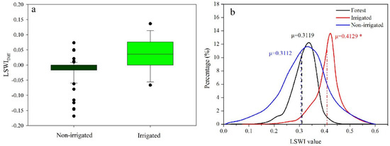
Figure 2.
The LSWI difference between non-irrigated (left) or irrigated (right) cropland pixels and their adjacent forests pixels. (a)The irrigated and non-irrigated cropland pixels were selected from field surveys. Histogram of LSWI values of adjacent forests pixels, irrigated croplands pixels and non-irrigated croplands pixels in northeastern China. (b)The Latin alphabet (μ) stands for the mean value of LSWI. The asterisk indicates the significant difference at the P < 0.01.
We examined the second assumption proposed in the previous section based on irrigation statistics and mean annual precipitation (MAP). We found a significant negative linear relationship between MAP and the LSWIDiff0 thresholds (difference in LSWI between irrigated cropland and forests) (P < 0.01) (Figure 3). The LSWIDiff0 thresholds decreased with increasing MAP, which indicated that larger a LSWI difference occurred in dry regions, affirming our second assumption. Therefore, we used regression to estimate the appropriate thresholds (LSWIDiff0) at all prefectures using MAP.
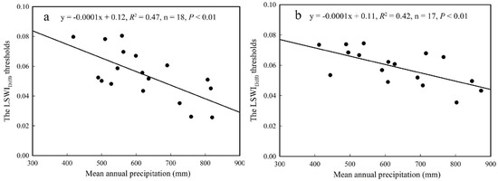
Figure 3.
The linear regression relationship between the (a) half of the area prefectures, (b) other half of the area prefectures LSWIDiff0 thresholds and the mean annual precipitation at the prefecture level in northeastern China.
The statistical data validated our method at the county, prefecture, and province levels, showing that the new method could accurately estimate irrigation areas compared to the statistical data over three scales (i.e., at the county, prefecture, and provincial levels) (Figure 4 and Table 1). The correlation coefficient (R2 values) between the identified irrigation areas and the statistical areas was 0.77 (Figure 4a) and 0.40 (Figure 4b) at the prefecture and county levels, respectively. Figure 4a provided the validation results of the second assumption. The identified irrigation areas were highly consistent with the statistical areas over the 18 prefecture prefectures used to develop the relationship between LSWIDiff0 and MAP, as shown Figure 3a. In addition, a good consistence between identified areas and statistical areas also was found over the remaining 17 prefecture prefectures (Figure 4a). At the province level, the relative errors of the identified irrigation areas were −26.41%, 26.34%, and 4.10% in Heilongjiang, Jilin, and Liaoning provinces, respectively (Table 1).

Figure 4.
Comparison of irrigated areas in Northeast China, as estimated by the proposed method and statistical areas at the prefecture (a) and county (b) levels. The dotted line is a 1:1 line. The black dots in Figure 4a indicate the 18 prefectures used for developing the relationship between LSWIDiff0 and MAP, and red dots indicate the remaining 17 prefectures for verification. Statistical area refers to the data of the irrigation area in a given administrative unit (such as a prefecture or a county) that were obtained from the statistical yearbooks for Heilongjiang, Jilin, and Liaoning.

Table 1.
Province-level comparison of estimated irrigated areas and statistical areas for 2016.
Based on the new method, we generated a map of irrigated fields in Northeast China in 2016 (Figure 5). Irrigated fields were distributed mainly on three alluvial plains (Songnen, Liaohe, and Sanjiang plains) and valleys along three rivers (the Songhua, Wusuli, and Heilongjiang Rivers). Due to the northward expansion of irrigated cropland over the past decade, Heilongjiang Province accounted for nearly 52.11% of the overall irrigation area in the three provinces, which is consistent with 2016 statistical data (Table 1) [43].

Figure 5.
Spatial distribution of estimated irrigated fields in Northeast China based on this method. Blue pixels indicate the irrigation areas.
5. Discussion
This study developed a new satellite-based method for identifying irrigation areas by comparing the satellite-based moisture index between croplands and adjacent forests. The results showed similar LSWI values for non-irrigated croplands and adjacent forests, but higher LSWI values for irrigated croplands (Figure 2b). Based on 123 surveyed sites, we compared the performance of this method with three other irrigation datasets: two global irrigation datasets (FAO/UF and IWMI) and an irrigation map of China derived by Zhu et al. [34] (see method). In general, the overall accuracy of our method was 77.24% and its kappa coefficient was 0.49; both measures were superior to the 47.15%, 62.60%, and 62.60% overall accuracies and 0.07, 0.23, and 0.11 kappa coefficients of the FAO/UF, IWMI, and Zhu datasets (Figure 6; Table 2). In general, the method identified correctly 26 irrigated samples out of total 47 irrigated samples, and identified correctly 76.67% non-irrigation samples (Figure 7; Table 2).
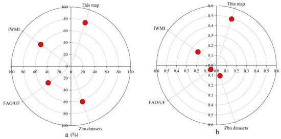
Figure 6.
Comparison of the performance of four datasets (this map, IWMI, FAO/UF, Zhu datasets) at 123 field sites. (a) overall accuracies (%); (b) Kappa coefficients.
Table 2.
Validation of four irrigation datasets at 123 field samples.
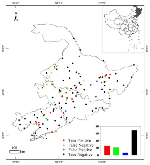
Figure 7.
Method validation proposed in this study at 123 field samples. True Positive: actual irrigated samples that were correctly classified as irrigated samples. True Negative: non-irrigated samples correctly classified as non-irrigated samples. False Positive: non-irrigated samples that were incorrectly labeled as irrigated samples. False Negative: irrigated samples that were incorrectly marked as non-irrigated samples. The inset indicates the site number of four categories.
Figure 3 showed the significant relationship between MAP and the LSWIDiff0 thresholds, which was used to identify the irrigation areas. Although there are some uncertainties, the relationship is statistically significant and indicates the reliable dependence of the threshold of LSWIDiff0 on MAP. Based on this relationship, we can identify the irrigation areas and avoid the systematic estimation errors compared to the constant threshold of LSWIDiff0. It is true that the estimation of irrigated areas performs well at the prefecture level (R2 = 0.77), rather than at the county level (R2=0.40) in Figure 4. Basically, there are large challenges in identifying the irrigation areas on a small scale (county) compared to on a large scale (prefecture). Many local environmental conditions will reduce the estimate accuracy [3,13,46]. For example, there are large estimation errors over the eastern regions of Jilin province because of the mountainous areas. Optical remotely sensed images in mountainous areas are subject to radiometric distortions induced by topographic effects, which need to be corrected before quantitative applications [47]. In addition, the moisture condition substantially changes with the topography and slope aspect, and precipitation is not the only factor which determines the moisture condition of croplands and the adjacent forests [48]. Therefore, further works need to improve the performance at mountainous areas.
The comparison suggests that the new irrigation map supports statistical areas at the prefecture-level and overall Northeast China. However, this study has underestimated Heilongjiang Province by 26.41% (Table 1). Major differences between irrigation patterns derived by the new map and the statistical data occurred in the Heilongjiang Farms & Land Reclamation Administration, which are mainly distributed in Heihe, Shuangyashan, and Jixi. Because the irrigation area data from the Heilongjiang Farms & Land Reclamation Administration are separately counted, they were not classified to prefectures, so statistics from this area were missing.
There are several limitations of this method which impacted its performance. First, this method identifies the irrigated croplands by comparing canopy moisture between cropland and adjacent forests. Therefore, it is important for the forests to be within a close enough distance for the forests to have the same precipitation as the croplands. Figure 8 shows that more than 50% of the croplands had forests within a distance of less than 25 km, which indicates that most croplands satisfy these conditions. However, in Songyuan and Baicheng of the Songnen Plain, the forests are relatively far away (>100km), and the precipitation conditions of croplands and its reference forests probably have large differences. Although this is only a small proportion (12%) [43,44,45], this will result in errors in the estimated irrigation areas.
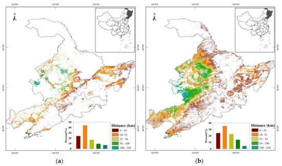
Figure 8.
Spatial distribution of the distance between cropland pixels and adjacent forests pixels in Northeast China. (a) the distance from forest to irrigated cropland pixels, (b) the distance from forest to non-irrigated cropland pixels.
Second, the method did not consider the differences of water storage between croplands and forests. In general, compared to the croplands, the adjacent forests green-up earlier [49,50]. Therefore, the forests can store more precipitation in the soil [51,52], which may result in the differences of soil moisture between the croplands and forests. In addition, previous studies showed that the capacity of plant transpiration and canopies to intercept water differs among ecosystems of the same leaf area index [53,54]. For example, at the same leaf area index (~2 m2 m−2), conifer forests typically store 20% of the precipitation, whereas the deciduous plants store 10% [54]. All crops in this study area are broadleaf, but the trees are broadleaf and needleleaf. The differences in the plant transpiration between croplands and forests may result in differences in soil moisture.
Third, this method relies on the regression relationship between LSWIDiff0 and MAP to identify irrigation areas (see method). In this study, we used regression coefficients, shown in Figure 3, over Northeast China, and the coefficients may change due to different climate backgrounds. Hence, if this method is applied to other regions, it is necessary to redefine the relationship between LSWIDiff0 and MAP.
Our method does not depend on field investigation and will be easy to popularize on a larger scale. The identification of irrigation pixels is consistent with actual irrigation samples in field surveys and statistical areas (Table 2). It is possible to supervise the distribution and the area of irrigation automatically using satellite-based datasets, avoiding visual interpretation [55,56,57] of high-resolution images [58] and much fieldwork, as well as substantially improving the method’s repeatability and applicability.
6. Conclusions
In this study, we developed a new method for identifying irrigation in cropland in northeastern China, based on the relationship between an area’s MAP and the LSWI difference between cropland and adjacent natural landscape pixels. We validated that the new method can be used to accurately map irrigation areas. In addition, we compared our method with three existing methods using site-based survey and county- to province-level statistical data. The results suggest that our method agrees with the patterns of irrigation distribution compared with the three current methods. Our method is a promising and effective tool for mapping irrigated regions. Moreover, it will be beneficial for studying water resource management and food security.
Author Contributions
Conceptualization, W.Y.; Data curation, X.Z.; Formal analysis, M.M.; Funding acquisition, W.Y.; Investigation, W.L. and J.D.; Methodology, K.X.; Resources, W.L.; Writing—original draft, K.X.; Writing—review & editing, W.Y.
Funding
This study was supported by National Key Basic Research Program of China (2016YFA0602701), National Youth Top-Notch Talent Support Program (2015-48), Changjiang Young Scholars Programme of China (Q2016161) and Training Project of Sun Yat-sen University (16lgjc53).
Acknowledgments
We thank Haicheng Zhang, Xiaoyuan Wang and Wenfang Xu for their help of data processing.
Conflicts of Interest
The authors declare no conflict of interest.
References
- Bruinsma, J. (Ed.) World Agriculture: Towards 2015/2030. An FAO Perspective; FAO and Earthscan Publ.: Rome, Italy; London, UK, 2003. [Google Scholar]
- Portmann, F.T.; Siebert, S.; Döll, P. MIRCA2000-Global monthly irrigated and rainfed crop areas around the year 2000: A new high-resolution data set for agricultural and hydrological modeling. Glob. Biogeochem. Cycles 2010, 24. [Google Scholar] [CrossRef]
- Yuan, W.; Liu, D.; Dong, W.; Liu, S.; Zhou, G.; Yu, G. Multiyear precipitation reduction strongly decreases carbon uptake over northern China. J. Geophys. Res. Biogeosciences 2014, 119, 881–896. [Google Scholar] [CrossRef]
- Ma, J.; Hoekstra, A.Y.; Wang, H.; Chapagain, A.K.; Wang, D. Virtual versus real water transfers within China. Philos. Trans. R. Soc. B 2006, 361, 835–842. [Google Scholar] [CrossRef]
- Veneman, A.M.; Jen, J.J.; Bosecker, R. Census of Agriculture-Farm and Ranch Irrigation Survey (2003), United States Department of Agriculture (USDA), National Agricultural Statistics Survey (NASS). Available online: http://www.usda.gov/nass/ (accessed on 4 April 2019).
- Yuan, W.; Liu, S.G.; Liu, W.; Zhao, S.Q.; Dong, W.J.; Tao, F.L.; Chen, M.; Lin, H. Opportunistic Market-Driven Regional Shifts of Cropping Practices Reduce Food Production Capacity of China. Earth’s Future 2018, 6, 634–642. [Google Scholar] [CrossRef]
- Food and Agriculture Organization of the United Nations (FAO): FAO Statistical Databases (FAOSTAT). Available online: http://faostat.fao.org/ (accessed on 4 April 2019).
- United Nations. United Nations Commission on Sustainable Development (UNCSD): Comprehensive Assessment of the Freshwater Resources of the World; Report E/CN.17/1997/9; Stockholm Environment Institute (SEI): Stockholm, Sweden.
- Popova, Z.; Kercheva, M. CERES model application for increasing preparedness to climate variability in agricultural planning—Risk analyses. Phys. Chem. Earth. 2005, 30, 117–124. [Google Scholar] [CrossRef]
- Shiklomanov, I.A. Appraisal and Assessment of World Water Resources. Water Int. 2000, 25, 11–32. [Google Scholar] [CrossRef]
- Ozdogan, M.; Yang, Y.; Allez, G.; Cervantes, C. Remote sensing of irrigated agriculture: Opportunities and challenges. Remote Sens. 2010, 2, 2274–2304. [Google Scholar] [CrossRef]
- Thenkabail, P.S.; Schull, M.; Turral, H. Ganges and Indus river basin land use/land cover (LULC) and irrigated area mapping using continuous streams of MODIS data. Remote Sens. Environ. 2005, 95, 317–341. [Google Scholar] [CrossRef]
- Ozdogan, M.; Gutman, G. A new methodology to map irrigated areas using multi-temporal MODIS and ancillary data: An application example in the continental US. Remote Sens. Environ. 2008, 112, 3520–3537. [Google Scholar] [CrossRef]
- Thenkabail, P.S.; Dheeravath, V.; Biradar, C.M.; Gangalakunta, O.R.P.; Noojipady, P.; Gurappa, C.; Velpuri, M.; Gumma, M.; Li, Y. Irrigated Area Maps and Statistics of India Using Remote Sensing and National Statistics. Remote Sens. 2009, 1, 50–67. [Google Scholar] [CrossRef]
- Dheeravath, V.; Thenkabail, P.S.; Chandrakantha, G.; Noojipady, P.; Reddy, G.P.O.; Biradar, C.M.; Gumma, M.K.; Velpuri, M. Irrigated areas of India derived using MODIS 500 m time series for the years 2001–2003. ISPRS J. Photogramm. Remote Sens. 2010, 65, 42–59. [Google Scholar] [CrossRef]
- Brown, J.F.; Pervez, M.S. Merging remote sensing data and national agricultural statistics to model change in irrigated agriculture. Agric. Syst. 2014, 127, 28–40. [Google Scholar] [CrossRef]
- Abuzar, M.; Mcallister, A.; Whitfield, D. Thresholds Derived from Landsat and ASTER Data in an Irrigation District of Australia. Photogramm. Eng. Remote Sens. 2015, 81, 229–238. [Google Scholar]
- Salmon, J.M.; Friedl, M.A.; Frolking, S.; Wisser, D.; Douglas, E.M. Global rain-fed, irrigated, and paddy croplands: A new high resolution map derived from remote sensing, crop inventories and climate data. Int. J. Appl. Earth Obs. Geoinf. 2015, 38, 321–334. [Google Scholar] [CrossRef]
- Biggs, T.W.; Thenkabail, P.S.; Gumma, M.K.; Scott, C.A.; Parthasaradhi, G.R.; Turral, H.N. Irrigated area mapping in heterogeneous landscapes with MODIS time series, ground truth and census data, Krishna Basin, India. Int. J. Remote Sens. 2006, 27, 4245–4266. [Google Scholar] [CrossRef]
- EL-Magd, I.A.; Tanton, T.W. Improvements in land use mapping for irrigated agriculture from satellite sensor data using a multi-stage maximum likelihood classification. Int. J. Remote Sens. 2003, 24, 4197–4206. [Google Scholar] [CrossRef]
- Simonneaux, V.; Duchemin, B.; Helson, D.; Er-Raki, S.; Olioso, A.; Chehbouni, A.G. The use of high-resolution image time series for crop classification and evapotranspiration estimate over an irrigated area in central Morocco. Int. J. Remote Sens. 2008, 29, 95–116. [Google Scholar] [CrossRef]
- Gumma, M.K.; Thenkabail, P.S.; Hideto, F.; Nelson, A.; Dheeravath, V.; Busia, D.; Rala, A. Mapping Irrigated Areas of Ghana Using Fusion of 30 m and 250 m Resolution Remote-Sensing Data. Remote Sens. 2011, 3, 816–835. [Google Scholar] [CrossRef]
- Löw, F.; Schorcht, G.; Michel, U.; Dech, S.; Conrad, C. Per-field crop classification in irrigated agricultural regions in middle Asia using random forest and support vector machine ensemble. Proc. SPIE 2012, 8538. [Google Scholar] [CrossRef]
- Lebourgeois, V.; Dupuy, S.; Vintrou, E.; Ameline, M.; Butler, S.; Bégué, A. A Combined Random Forest and OBIA Classification Scheme for Mapping Smallholder Agriculture at Different Nomenclature Levels Using Multisource Data (Simulated Sentinel-2 Time Series, VHRS and DEM). Remote Sens. 2017, 9, 259. [Google Scholar] [CrossRef]
- Bégué, A.; Arvor, D.; Bellon, B.; Betbeder, J.; Abelleyra, D.D.; Ferraz, R.P.D. Remote Sensing and Cropping Practices: A Review. Remote Sens. 2018, 10, 99. [Google Scholar] [CrossRef]
- Brown, J.C.; Kastens, J.H.; Coutinho, A.C.; Victoria, D.D.C.; Bishop, C.R. Classifying multiyear agricultural land use data from Mato Grosso using time-series MODIS vegetation index data. Remote Sens. Environ. 2013, 130, 39–50. [Google Scholar] [CrossRef]
- Liu, W.; Dong, J.; Xiang, K.; Wang, S.; Han, W.; Yuan, W. A sub-pixel method for estimating planting fraction of paddy rice in Northeast China. Remote Sens. Environ. 2018, 205, 305–314. [Google Scholar] [CrossRef]
- Kamthonkiat, D.; Honda, K.; Turral, H.; Tripathi, N.; Wuwongse, V. Discrimination of irrigated and rainfed rice in a tropical agricultural system using SPOT VEGETATION NDVI and rainfall data. Int. J. Remote Sens. 2005, 26, 2527–2547. [Google Scholar] [CrossRef]
- Chen, Y.L.; Lu, D.S.; Luo, L.F.; Pokhrel, Y.; Deb, K.; Huang, J.F.; Ran, Y.H. Detecting irrigation extent, frequency, and timing in a heterogeneous arid agricultural region using MODIS time series, Landsat imagery, and ancillary data. Remote Sens. Environ. 2018, 204, 197–211. [Google Scholar] [CrossRef]
- Döll, P.; Siebert, S.A. Digital Global Map of Irrigated Areas. ICID J. 1999, 49, 55–66. [Google Scholar]
- Siebert, S.; Henrich, V.; Frenken, K.; Burke, J. Update of the Digital Global Map of Irrigation Areas to Version 5.0; FAO: Rome, Italy, 2013. [Google Scholar]
- Thenkabail, P.S.; Biradar, C.M.; Noojipady, P.; Dheeravath, V.; Li, Y.; Velpuri, M.; Gumma, M.; Gangalakunta, O.R.P.; Turral, H.; Cai, X. Global irrigated area map (GIAM), derived from remote sensing, for the end of the last millennium. Int. J. Remote Sens. 2009, 30, 3679–3733. [Google Scholar] [CrossRef]
- Arino, O.; Gross, D.; Ranera, F.; Leroy, M.; Bicheron, P.; Brockman, C. GlobCover: ESA service for Global Land Cover from MERIS. In Proceedings of the 2007 IEEE International Geoscience and Remote Sensing Symposium, Barcelona, Spain, 23–28 July 2007. [Google Scholar]
- Zhu, X.; Zhu, W.; Zhang, J.; Pan, Y. Mapping Irrigated Areas in China From Remote Sensing and Statistical Data. IEEE Appl. Earth Obs. Remote Sens. 2015, 7, 4490–4504. [Google Scholar] [CrossRef]
- National Bureau of Statistics of China. China Statistical Yearbook 2017; China Statistics Press: Beijing, China, 2017. [Google Scholar]
- Wu, P.T.; Jin, J.M.; Zhao, X.N. Impact of climate change and irrigation technology advancement on agricultural water use in China. Clim. Change 2010, 100, 797–805. [Google Scholar] [CrossRef]
- Jin, N.; Tao, B.; Ren, W.; Feng, M.; Sun, R.; He, L.; Zhuang, W.; Yu, Q. Mapping Irrigated and Rainfed Wheat Areas Using Multi-Temporal Satellite Data. Remote Sens. 2016, 8, 207. [Google Scholar] [CrossRef]
- Boschetti, M.; Nutini, F.; Manfron, G.; Brivio, P.A.; Nelson, A. Comparative Analysis of Normalised Difference Spectral Indices Derived from MODIS for Detecting Surface Water in Flooded Rice Cropping Systems. PLoS ONE 2014, 9, e88741. [Google Scholar] [CrossRef] [PubMed]
- Chandrasekar, K.; Sesha Sai, M.V.R.; Roy, P.S.; Dwevedi, R.S. Land Surface Water Index (LSWI) response to rainfall and NDVI using the MODIS Vegetation Index product. Int. J. Remote Sens. 2010, 31, 3987–4005. [Google Scholar] [CrossRef]
- Xiao, X.; Boles, S.; Liu, J.; Zhuang, D.; Frolking, S.; Li, C.; Salas, W.; Moore, B. Mapping paddy rice agriculture in southern China using multi-temporal MODIS images. Remote Sens. Environ. 2005, 95, 480–492. [Google Scholar] [CrossRef]
- Chen, J.; Jönsson, P.; Tamura, M.; Gu, Z.; Matsushita, B.; Eklundh, L. A simple method for reconstructing a high-quality NDVI time-series data set based on the Savitzky-Golay filter. Remote Sens. Environ. 2004, 91, 332–344. [Google Scholar] [CrossRef]
- Yuan, W.; Xu, B.; Chen, Z.; Xia, J.; Xu, W.; Chen, Y. Validation of China-wide interpolated daily climate variables from 1960 to 2011. Theor. Appl. Climatol. 2015, 119, 689–700. [Google Scholar] [CrossRef]
- Heilongjiang Stastical Bureau. Heilongjiang Statistical Yearbook in 2016; China Statistics Press: Beijing, China, 2016. [Google Scholar]
- Jilin Statistical Bureau. Jilin Statistical Yearbook in 2016; China Statistics Press: Beijing, China, 2016. [Google Scholar]
- Liaoning Statistical Bureau. Liaoning Statistical Yearbook in 2016; China Statistics Press: Beijing, China, 2016. [Google Scholar]
- Wardlow, B.D.; Egbert, S.L. Large-area crop mapping using time-series MODIS 250 m NDVI data: An assessment for the US Central Great Plains. Remote Sens. Environ. 2008, 112, 1096–111. [Google Scholar] [CrossRef]
- Li, A.; Wang, Q.; Bian, J.; Lei, G. An Improved Physics-Based Model for Topographic Correction of Landsat TM Images. Remote Sens. 2015, 7, 6296–6319. [Google Scholar] [CrossRef]
- Qiu, Y.; Fu, B.; Wang, J.; Chen, L. Soil moisture variation in relation to topography and land use in a hillslope catchment of the Loess Plateau, China. J. Hydrol. 2001, 240, 243–263. [Google Scholar] [CrossRef]
- Wen, Z.; Wu, S.; Chen, J.; Lü, M.Q. NDVI indicated long-term interannual changes in vegetation activities and their responses to climatic and anthropogenic factors in the Three Gorges Reservoir Region, China. Sci. Total Environ. 2017, 574, 947–959. [Google Scholar] [CrossRef]
- Peng, D.; Wu, C.; Li, C.; Zhang, X.; Liu, Z.; Ye, H. Spring green-up phenology products derived from MODIS NDVI and EVI: Intercomparison, interpretation and validation using National Phenology Network and AmeriFlux observations. Ecol. Indic. 2017, 77, 323–336. [Google Scholar] [CrossRef]
- Hopmans, J.W.; Bales, R.C.; O’Geen, A.T.; Meadows, M.; Hartsough, P.C.; Kirchner, P.; Hunsaker, C.T.; Beaudette, D.; Bales, R.C. Soil moisture response to snowmelt and rainfall in a sierra nevada mixed-conifer forest. Vadose Zone J. 2012, 11, 786–799. [Google Scholar] [CrossRef]
- Mcintyre, P.J.; Thorne, J.H.; Dolanc, C.R.; Flint, A.L.; Flint, L.E.; Kelly, M. Twentieth-century shifts in forest structure in California: Denser forests, smaller trees, and increased dominance of oaks. Proc. Natl. Acad. Sci. USA 2015, 112, 1458–1463. [Google Scholar] [CrossRef]
- Szilagyi, J. Can a vegetation index derived from remote sensing be indicative of areal transpiration? Ecol. Model. 2000, 127, 65–79. [Google Scholar] [CrossRef]
- Waring, R.H.; Running, S.W. Forest Ecosystems: Analysis at Multiple Scales; Academic Press: New York, NY, USA, 1998. [Google Scholar]
- Zhong, L.; Gong, P.; Biging, G.S. Efficient corn and soybean mapping with temporal extendability: A multi-year experiment using Landsat imagery. Remote Sens. Environ. 2014, 140, 1–13. [Google Scholar] [CrossRef]
- Dong, J.; Xiao, X.; Kou, W.; Qin, Y.; Zhang, G.; Li, L.; Jin, C.; Zhou, Y.; Wang, J.; Biradar, C. Tracking the dynamics of paddy rice planting area in 1986–2010 through time series Landsat images and phenology-based algorithms. Remote Sens. Environ. 2015, 160, 99–113. [Google Scholar] [CrossRef]
- Zhu, C.; Lu, D.; Victoria, D.; Dutra, L. Mapping Fractional Cropland Distribution in Mato Grosso, Brazil Using Time Series MODIS Enhanced Vegetation Index and Landsat Thematic Mapper Data. Remote Sens. 2015, 8, 22. [Google Scholar] [CrossRef]
- Beltrán, C.M.; Belmonte, A.C. Irrigated crop area estimation using Landsat TM imagery in La Mancha, Spain. ISPRS J. Photogramm. Remote Sens. 2001, 67, 1177–1184. [Google Scholar]


© 2019 by the authors. Licensee MDPI, Basel, Switzerland. This article is an open access article distributed under the terms and conditions of the Creative Commons Attribution (CC BY) license (http://creativecommons.org/licenses/by/4.0/).