A Three-Stage Hybrid Learning Framework for Sustainable Multi-Energy Load Forecasting in Park-Level Integrated Energy Systems

Abstract

Accurate multi-energy load forecasting is essential for the low-carbon, efficient, and resilient operation of park-level Integrated Energy Systems (PIESs), where cooling, heating, and electricity networks interact closely and increasingly incorporate renewable energy resources. However, forecasting in such systems remains challenging due to complex cross-energy coupling, high-dimensional feature interactions, and pronounced nonlinearities under diverse meteorological and operational conditions. To address these challenges, this study develops a novel three-stage hybrid forecasting framework that integrates Recursive Feature Elimination with Cross-Validation (RFECV), a Multi-Task Long Short-Term Memory network (MTL-LSTM), and Random Forest (RF). In the first stage, RFECV performs adaptive and interpretable feature selection, ensuring robust model inputs and capturing meteorological drivers relevant to renewable energy dynamics. The second stage employs MTL-LSTM to jointly learn shared temporal dependencies and intrinsic coupling relationships among multiple energy loads. The final RF-based residual correction enhances local accuracy by capturing nonlinear residual patterns overlooked by deep learning. A real-world case study from an East China PIES verifies the superior predictive performance of the proposed framework, achieving mean absolute percentage errors of 4.65%, 2.79%, and 3.01% for cooling, heating, and electricity loads, respectively—substantially outperforming benchmark models. These results demonstrate that the proposed method offers a reliable, interpretable, and data-driven solution to support refined scheduling, renewable energy integration, and sustainable operational planning in modern multi-energy systems.

1. Introduction

Park-level Integrated Energy Systems (PIESs) enable cascade utilization of electricity, heating, and cooling through the coupling and conversion of multiple energy flows, thereby achieving overall system optimization. Although multi-energy complementarity significantly enhances energy efficiency, it simultaneously introduces a new set of technical challenges. On one hand, the strong coupling among different energy loads makes them difficult to predict independently and accurately; on the other hand, load sequences are influenced by complex interactions among meteorological conditions, equipment operating states, and spatiotemporal dependencies, exhibiting pronounced nonlinear and time-varying characteristics. Consequently, conventional forecasting methods struggle to cope with the combined challenges of high feature dimensionality, intricate coupling mechanisms, and strong nonlinearity. These challenges necessitate the development of new forecasting frameworks capable of deeply integrating temporal features with coupling mechanisms to support efficient operation and refined control of PIESs.

Traditional short-term load forecasting methods primarily include time series analysis and regression techniques. Time series methods utilize intrinsic temporal patterns in historical data for load forecasting. For short-term load forecasting, traditional approaches primarily include time-series analysis and regression-based methods. Time-series models exploit intrinsic temporal patterns within historical data to predict future loads. For example, the Autoregressive Integrated Moving Average (ARIMA) model and its double-seasonal extension (DSARIMA) characterize short-term variations by leveraging the continuity and periodic structure of load sequences [1,2]. However, because these models rely on linear assumptions, they often struggle to capture strong nonlinear patterns arising from weather fluctuations, holiday schedules, and user behavior. Their adaptability is further limited when confronted with the intricate coupling mechanisms inherent in multi-energy flow scenarios [3]. In contrast, machine learning methods—such as Support Vector Machines (SVMs), Artificial Neural Networks (ANNs), and RF—have been widely adopted due to their ability to model nonlinear relationships in short-term load forecasting. For instance, SVMs employ kernel functions to map load data into high-dimensional feature spaces and thereby capture nonlinear dependencies [4]. Nevertheless, as renewable energy penetration increases, demand-side interactions intensify, and multi-source coupling effects become more pronounced, shallow learning models face growing challenges in capturing long-range temporal dependencies and high-level feature interactions. Consequently, their forecasting accuracy and generalization capability tend to plateau under complex and strongly coupled load conditions [5,6]. The rise of deep learning offers new pathways for improving forecasting accuracy. Long Short-Term Memory (LSTM) networks, which alleviate the vanishing gradient problem and effectively capture temporal dependencies, have become a mainstream method. By extracting temporal features from power load sequences, LSTMs have achieved satisfactory results in ultra-short-term load forecasting [7]. Convolutional Neural Networks (CNNs) also excel in high-dimensional feature extraction; for instance, 1D-CNNs can mine local characteristics in load data and are suitable for load modeling under multiple influencing factors [8]. Nevertheless, individual deep learning models possess inherent shortcomings: LSTMs are prone to forgetting critical information when input sequences are excessively long [9]; CNNs are ineffective at modeling long-range dependencies in sequential data [10]; and model performance depends heavily on hyperparameter tuning and input feature quality, resulting in insufficient robustness [11]. To overcome the limitations of single models, hybrid models have become a key research focus. One approach uses Complete Ensemble Empirical Mode Decomposition with Adaptive Noise (CEEMDAN) to decompose load sequences, reconstructs components via sample entropy, and subsequently applies LSTM for forecasting. This method effectively addresses the autocorrelation issue of decomposed components and reduces the RMSE by approximately 30% compared to standard LSTM [12]. Another hybrid model combining CNNs, LSTM, and an attention mechanism uses CNNs for high-dimensional feature extraction, LSTM to capture temporal patterns, and attention to optimize information weighting. This architecture improved forecasting accuracy by 5.7–7.3% compared to a standalone LSTM in a Combined Heat and Power (CHP) system [13]. Furthermore, hybrid frameworks integrating stacked ensemble learning and deep reinforcement learning have shown potential for enhancing forecasting stability in distributed IES [14]. Such hybrid models, by combining the strengths of different algorithms, demonstrate superior performance in modeling nonlinear load characteristics. However, some designs suffer from structural complexity and high computational cost, hindering their application to real-time forecasting in large-scale parks [15].

While the aforementioned hybrid models focus primarily on improving the forecasting accuracy of individual load sequences, explicitly modeling the coupling relationships among multiple energy flows remains a more fundamental and intrinsic challenge for PIES. Some studies continue to adopt the traditional paradigm of separately modeling cooling, heating, and electricity loads—for example, regional thermal load forecasting based on multiple linear regression [16] and cooling load prediction using nonlinear autoregressive neural networks [17]. Although such approaches are methodologically straightforward and easy to implement, they overlook the synergistic interactions and physical constraints inherent among multi-energy flows, often resulting in system-level forecasting deviations. To incorporate energy-flow coupling information, several indirect modeling strategies have been explored. One approach introduces other energy loads as auxiliary inputs through feature engineering—such as incorporating thermal and cooling load data into electricity load forecasting models to implicitly reflect inter-load dependencies [18]. Another strategy constructs single-task, multi-output models capable of forecasting multiple loads within a unified framework; however, substantial differences in load magnitudes, dynamic behaviors, and variation patterns frequently cause training instability and poor convergence performance [19]. Multi-Task Learning (MTL) provides a promising alternative for addressing these challenges. By learning shared representations across tasks while preserving task-specific output branches, MTL can explicitly capture coupling mechanisms among multiple loads. For instance, deep multi-task architectures combining Deep Belief Networks (DBNs) with multi-task regression layers achieve an average accuracy improvement of approximately 2.7% over single-task models [20]. Similarly, integrating MTL with Least-Squares Support Vector Machines (LSSVMs) and optimizing cross-task weights yields an 18.6% enhancement in forecasting accuracy [21]. In addition, a “shared autoregressive–specific dual-dilated convolutional self-attention” architecture has been proposed, in which a shared AR module extracts linear correlations among turbines while task-specific attention modules capture nonlinear turbine-level features, effectively addressing power forecasting challenges for newly constructed wind farms with limited data [22]. These studies collectively demonstrate the advantages of MTL in explicitly modeling temporal coupling relationships among multi-energy loads. Nevertheless, existing MTL frameworks often fail to adequately prioritize different load tasks, limiting their ability to satisfy the differentiated forecasting requirements of core loads [23]. In recent years, more forward-looking deep learning architectures have been widely applied to load forecasting tasks in IES and regional energy networks. Graph Neural Networks (GNNs) and their spatiotemporal extensions—such as ST-GCN and GAT-based models—explicitly leverage the topological structure of park-level energy networks or multi-building clusters, demonstrating strong capability in modeling cross-regional energy flow interactions and consistently outperforming traditional sequence-based models in regional IES load forecasting [24]. Meanwhile, Transformer-based architectures, benefiting from self-attention mechanisms for long-range temporal dependency modeling, have achieved remarkable progress in tasks such as electricity load forecasting and net-load prediction [25]. Ensemble frameworks that integrate gradient boosting models with deep neural networks have also shown improved robustness and adaptability in residential demand response and building energy consumption forecasting [26]. Beyond load forecasting itself, deep learning methods have also been extensively adopted in renewable energy prediction, providing crucial support for developing more sustainable park-level energy systems. For example, hybrid models combining graph convolutional networks and recurrent neural networks have been employed for short-term photovoltaic and wind power forecasting, demonstrating clear advantages in distributed energy scenarios [27]. Recent studies on hybrid renewable energy systems (HRES) have further integrated LSTM, Bi-LSTM, and MLP models to perform multi-source forecasting of solar, wind, and biomass generation, and have combined such forecasts with load prediction to support energy mix optimization, operational strategy design, and carbon emission assessment [28]. However, as the variability of renewable energy, the coupling of multi-energy flows, and the complexity of system operation mechanisms continue to increase, these models must handle more diverse and structurally complex input information in practical applications, imposing higher requirements on the forecasting framework.

Whether in advanced hybrid models or MTL frameworks, high-quality feature inputs remain fundamental to achieving reliable predictive performance. As the range of influencing factors continues to expand, load forecasting is increasingly challenged by a rapidly growing feature dimensionality. Meteorological variables, user behavior patterns, equipment operating states, and other load attributes collectively form a high-dimensional input space—particularly in renewable energy scenarios such as photovoltaic (PV) and wind power systems, where irradiance, humidity, wind speed, and cloud cover exhibit strong volatility and complex coupling. Directly feeding such features into forecasting models not only results in substantial computational overhead but may also introduce redundant or noisy variables, ultimately reducing model generalizability [29]. Traditional feature selection methods exhibit clear limitations. Pearson-correlation-based filtering can only capture linear relationships and is incapable of modeling the more common nonlinear interactions between loads and environmental or behavioral variables [30]. Experience-driven feature selection is inherently subjective and fails to adapt to evolving system characteristics [31]. One-time static feature sets also struggle to accommodate the dynamic changes in operational conditions [32]. These limitations are particularly evident in PV power forecasting; for example, recent findings in solar power plant studies show that different combinations of meteorological inputs can significantly affect forecasting accuracy, and fixed feature sets are often unable to reflect rapidly changing weather conditions [33]. To address these shortcomings, automated and dynamic feature selection mechanisms have gained increasing attention. The integration of Recursive Feature Elimination (RFE) with deep Bidirectional Long Short-Term Memory (BiLSTM) networks enables continuous updates to feature importance, thereby improving the model’s sensitivity to time-varying factors [34]. Multi-layer weather classification combined with hierarchical regression has also been developed to reduce redundant features in PV scenarios by structuring inputs according to weather conditions [35]. Meanwhile, more advanced feature expansion strategies have emerged. Deep spatiotemporal attention models, for instance, explicitly capture temporal and spatial dependencies between loads and meteorological variables, offering greater adaptability to complex multi-energy coupling characteristics than traditional Copula-based approaches [36]. The fusion of Spatiotemporal Graph Attention Networks (ST-GAT) with multi-stage feature selection further demonstrates strong potential in dynamic feature identification for commercial building cooling load forecasting [37]. Additionally, Bayesian-optimized LSTM architectures that jointly refine input structures and hyperparameters have shown enhanced robustness and sensitivity to key meteorological features in PV power forecasting [38]. Despite these advances, achieving an optimal balance between real-time feature selection efficiency and forecasting accuracy in practical PIESs remains an essential challenge for future research.

In summary, while existing research offers diverse methodological approaches for IES load forecasting, several limitations persist for practical park-level applications: hybrid models demonstrate insufficient capability in explicitly addressing multi-energy coupling and dynamic feature selection, while nonlinear components within forecasting residuals remain inadequately compensated. To systematically overcome these challenges, this paper proposes a hybrid forecasting framework that intelligently integrates RFECV, an MTL-LSTM network, and RF. The proposed framework employs a structured three-stage methodology: initially, RFECV performs dynamic feature selection; subsequently, MTL-LSTM simultaneously forecasts multiple load types while capturing their coupling relationships through shared mechanisms; finally, RF is implemented to correct the residuals generated by the primary forecasting model. This modular, phased strategy is designed to significantly enhance both forecasting accuracy and robustness for PIES, while maintaining desirable model interpretability.

2. Materials and Methods

2.1. IES Load Characteristic Analysis

PIESs serve as complex multi-energy networks in which electricity, heat, and cooling interact through coupling and conversion. As illustrated in Figure 1, a typical commercial-park PIES architecture achieves the coupling, conversion, and coordination of multiple energy forms through key energy conversion and storage devices, including heat pumps, electric chillers, absorption chillers, and energy storage units.

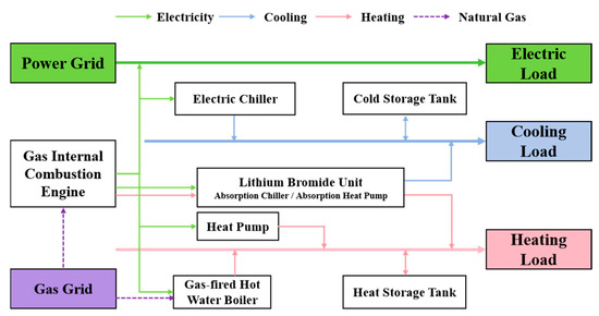
Figure 1. Typical IES architecture of a commercial park.

In general, the load of a commercial PIES exhibits pronounced temporal and nonlinear characteristics, with variations jointly driven by multiple factors such as meteorological conditions, human-flow fluctuations, and scheduled commercial activities within the park [39,40,41,42]. Compared with conventional commercial buildings, the system investigated in this study possesses a distinctive feature: its energy consumption is primarily driven by meteorological conditions and prearranged commercial activity schedules, while demonstrating low sensitivity to real-time changes in human flow. This arises from its operation mode, which incorporates reservation and flow control mechanisms to maintain a relatively stable number of occupants within the park, thereby mitigating the impact of instantaneous pedestrian fluctuations on the overall system load.

2.2. Expert-Knowledge-Guided RFECV Feature Selection

In PIES load forecasting, the input features typically span multiple dimensions, including multi-energy coupling data, meteorological parameters, and historical load sequences. While a high-dimensional feature space provides abundant information, it may also introduce redundancy and noise, adversely affecting model performance and computational efficiency. To address this issue, this study proposes an expert-knowledge-guided RFECV strategy. The approach embeds time-series cross-validation into the recursive-elimination process to evaluate the performance of feature subsets, thereby accommodating the temporal dependencies inherent in the data and preventing information leakage. Ultimately, it ensures both the effectiveness and efficiency of the selected feature set while preserving physical interpretability.

To account for the temporal structure of the dataset and to prevent information leakage, a TimeSeriesSplit cross-validation scheme is adopted. Let the chronologically ordered dataset be denoted as

$$\{\left({\mathrm{x}}_{\mathrm{t}},{\mathrm{y}}_{\mathrm{t}}\right){\}}_{\mathrm{t}=1}^{\mathrm{N}}$$

(1)

where ${\mathrm{x}}_{\mathrm{t}}\in {\mathrm{R}}^{\mathrm{D}}$ denotes the D-dimensional input feature vector at hour t, and ${\mathrm{y}}_{\mathrm{t}}={\left[{\mathrm{y}}_{1,t},{\mathrm{y}}_{2,t},{\mathrm{y}}_{3,t}\right]}^{\mathrm{T}}$ represents the cooling load, heating load, and electricity load.

For a total of K folds, the training and validation index sets for the r-th fold are defined as

$${\mathrm{I}}_{\mathrm{t}\mathrm{r}}^{\left(\mathrm{r}\right)}=\{1,\dots ,\lfloor {\displaystyle \frac{\mathrm{r}\mathrm{N}}{\mathrm{K}+1}}\rfloor \}$$

(2)

$${\mathrm{I}}_{\mathrm{v}\mathrm{a}\mathrm{l}}^{\left(\mathrm{r}\right)}=\left\{\lfloor {\displaystyle \frac{\mathrm{r}\mathrm{N}}{\mathrm{K}+1}}\rfloor +1,\dots ,\lfloor {\displaystyle \frac{(\mathrm{r}+1)\mathrm{N}}{\mathrm{K}+1}}\rfloor \right\}$$

(3)

Accordingly, the training and validation subsets are

$${\mathrm{D}}_{\mathrm{t}\mathrm{r}}^{\left(\mathrm{r}\right)}=\left\{\left({\mathrm{x}}_{\mathrm{t}},{\mathrm{y}}_{\mathrm{t}}\right)\right|\mathrm{t}\in {\mathrm{I}}_{\mathrm{t}\mathrm{r}}^{\left(\mathrm{r}\right)}\}$$

(4)

$${\mathrm{D}}_{\mathrm{v}\mathrm{a}\mathrm{l}}^{\left(\mathrm{r}\right)}=\left\{\left({\mathrm{x}}_{\mathrm{t}},{\mathrm{y}}_{\mathrm{t}}\right)\right|\mathrm{t}\in {\mathrm{I}}_{\mathrm{v}\mathrm{a}\mathrm{l}}^{\left(\mathrm{r}\right)}\}$$

(5)

For any candidate feature subset S ⊆ Sfull, the time-series cross-validation loss is computed as

$$\mathrm{J}\left(\mathrm{S}\right)={\displaystyle \frac{1}{\mathrm{K}}}\sum _{\mathrm{r}=1}^{\mathrm{K}}{\mathrm{L}}_{\mathrm{v}\mathrm{a}\mathrm{l}}^{\left(\mathrm{r}\right)}\left(\mathrm{S}\right)$$

(6)

where ${\mathrm{L}}_{\mathrm{v}\mathrm{a}\mathrm{l}}^{\left(\mathrm{r}\right)}\left(\mathrm{S}\right)$ denotes the mean squared error (MSE) obtained using only the features in S on validation fold r.

A RF regressor is used as the base estimator for feature importance evaluation. For the t-th decision tree in the forest, the importance of feature j is quantified using the variance reduction achieved at split nodes [43]:

$${\mathrm{I}}_{\mathrm{t}}\left(\mathrm{j}\right)=\sum _{\mathrm{m}\in {\mathrm{M}}_{\mathrm{t}}\left(\mathrm{j}\right)}{\mathsf{\omega }}_{\mathrm{m}}\left[\mathrm{V}\mathrm{a}\mathrm{r}\left({\mathrm{D}}_{\mathrm{m}}\right)-\left({\displaystyle \frac{\left|{\mathrm{D}}_{\mathrm{m}}^{\mathrm{L}}\right|}{\left|{\mathrm{D}}_{\mathrm{m}}\right|}}\mathrm{V}\mathrm{a}\mathrm{r}\left({\mathrm{D}}_{\mathrm{m}}^{\mathrm{L}}\right)+{\displaystyle \frac{\left|{\mathrm{D}}_{\mathrm{m}}^{\mathrm{R}}\right|}{\left|{\mathrm{D}}_{\mathrm{m}}\right|}}\mathrm{V}\mathrm{a}\mathrm{r}\left({\mathrm{D}}_{\mathrm{m}}^{\mathrm{R}}\right)\right)\right]$$

(7)

and the aggregated importance over all T trees is

$$\mathrm{I}\left(\mathrm{j}\right)={\displaystyle \frac{1}{\mathrm{T}}}\sum _{\mathrm{t}=1}^{\mathrm{T}}{\mathrm{I}}_{\mathrm{t}}\left(\mathrm{j}\right)$$

(8)

where ${\mathrm{M}}_{\mathrm{t}}\left(\mathrm{j}\right)$ denotes the collection of internal nodes in the t-th tree where feature j is used to perform splits. For each such node $\mathrm{m}\in {\mathrm{M}}_{\mathrm{t}}\left(\mathrm{j}\right)$, ${\mathrm{D}}_{\mathrm{m}}$ represents the parent node sample set, while ${\mathrm{D}}_{\mathrm{m}}^{\mathrm{L}}$ and ${\mathrm{D}}_{\mathrm{m}}^{\mathrm{R}}$ denote its left-child and right-child subsets, respectively; $|·|$ denotes the cardinality of the corresponding sample set. The term ${\mathsf{\omega }}_{\mathrm{m}}=\left|{\mathrm{D}}_{\mathrm{m}}\right|/\mathrm{N}$ is the normalized node weight, ensuring that node contributions are proportional to their sample sizes. The operator $\mathrm{V}\mathrm{a}\mathrm{r}(·)$ denotes the sample variance of the target load values, reflecting the impurity of each node [44].

Let P denote the set of expert-anchored features that must always be retained, and let ${\mathrm{S}}^{\left(0\right)}={\mathrm{S}}_{\mathrm{f}\mathrm{u}\mathrm{l}\mathrm{l}}\setminus \mathrm{P}$ be the set of features subject to elimination. At iteration r, the feature with the lowest importance is removed according to

$${\mathrm{j}}^{\mathrm{*}}=\arg \underset{\mathrm{j}\in {\mathrm{S}}^{\left[\mathrm{r}\right]}}{\min }\mathrm{I}\left(\mathrm{j}\right)$$

(9)

$${\mathrm{S}}^{(\mathrm{r}+1)}={\mathrm{S}}^{\left(\mathrm{r}\right)}\setminus \left\{{\mathrm{j}}^{\mathrm{*}}\right\}$$

(10)

For each subset ${\mathrm{S}}^{\left(\mathrm{r}\right)}$, the cross-validation loss $\mathrm{J}\left({\mathrm{S}}^{\left(\mathrm{r}\right)}\right)$ is computed via (6).

The optimal feature subset is then identified as

$${\mathrm{S}}^{\mathrm{o}\mathrm{p}\mathrm{t}}=\arg \underset{{\mathrm{S}}^{\left(\mathrm{r}\right)}}{\min }\mathrm{J}\left({\mathrm{S}}^{\left(\mathrm{r}\right)}\right)$$

(11)

The final selected feature set is constructed by combining the expert-anchored features and the optimal subset obtained from RFECV:

$${\mathrm{S}}^{\mathrm{f}\mathrm{i}\mathrm{n}\mathrm{a}\mathrm{l}}=\mathrm{P}\cup {\mathrm{S}}^{\mathrm{o}\mathrm{p}\mathrm{t}},\hspace{1em}{\tilde{\mathrm{x}}}_{\mathrm{t}}\in {\mathrm{R}}^{{\mathrm{D}}_{\mathrm{s}}}$$

(12)

where ${\mathrm{D}}_{\mathrm{s}}$ denotes the dimension of the final selected feature vector ${\tilde{\mathrm{x}}}_{\mathrm{t}}$.

This expert-knowledge-guided RFECV framework selects features that are both physically meaningful and statistically robust, thereby enhancing the interpretability and predictive capacity of the subsequent hybrid MTL-LSTM-RF forecasting model.

2.3. Construction of the MTL-LSTM-RF Forecasting Model

To precisely characterize the multi-source coupling characteristics and temporal evolution patterns of cooling, heating, and electricity loads in PIES, this study develops a hybrid forecasting model that integrates an MTL-LSTM network with a RF-based residual correction mechanism. Building upon the results of feature selection, the proposed MTL-LSTM-RF model adopts a two-stage strategy—deep temporal modeling followed by residual compensation—to achieve coordinated and high-accuracy forecasts across the three types of energy loads.

In the first stage, the MTL-LSTM serves as the primary forecasting architecture. A shared LSTM layer learns common temporal dynamics and energy-flow coupling relationships among the different loads, while task-specific output layers generate the initial predictions for cooling, heating, and electricity loads, respectively. In the second stage, to mitigate the accuracy degradation of the primary model when facing abrupt disturbances and local non-stationary patterns, an RF-based residual correction module is introduced. This module takes the preliminary predictions from the MTL-LSTM together with a set of screened key input features as inputs to learn the nonlinear residual structures not fully captured by the primary model, thereby performing error compensation and refining the final outputs.

2.3.1. Multi-Task Learning Forecasting Layer

The MTL-LSTM network serves as the primary forecasting structure of the proposed hybrid model. Compared with training independent single-task models, the MTL-LSTM simultaneously learns shared temporal dependencies and energy flow coupling relationships, while task-specific output layers capture the unique dynamics of each load type. This approach enhances generalization and coordination among the prediction tasks for cooling, heating, and electricity loads within the PIES, as illustrated in Figure 2.

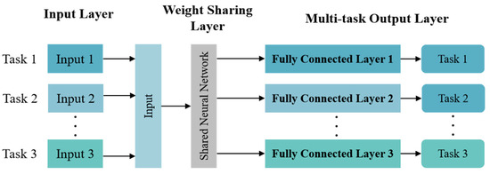
Figure 2. Conceptual framework of the MTL architecture.

Let ${\tilde{\mathrm{x}}}_{\mathrm{t}}\in {\mathrm{R}}^{{\mathrm{D}}_{\mathrm{s}}}$ denote the selected input feature vector at hour t, where ${\mathrm{D}}_{\mathrm{s}}$ is the dimension of the screened feature set. A look-back window of length T is constructed as

$${\mathrm{X}}_{\mathrm{t}}=[{\tilde{\mathrm{x}}}_{\mathrm{t}-\mathrm{T}+1},\dots ,{\tilde{\mathrm{x}}}_{\mathrm{t}}]$$

(13)

The shared LSTM layer processes the input sequence $\{{\tilde{\mathrm{x}}}_{\mathrm{t}},\mathrm{T}+1,\dots ,{\tilde{\mathrm{x}}}_{\mathrm{t}}\}$ and updates its internal states using the standard gating mechanism. At each time step t, the forget gate ${\mathrm{f}}_{\mathrm{t}}$, input gate ${\mathrm{i}}_{\mathrm{t}}$, candidate cell state ${\tilde{\mathrm{c}}}_{\mathrm{t}}$, cell state ${\mathrm{c}}_{\mathrm{t}}$, output gate ${\mathrm{o}}_{\mathrm{t}}$, and hidden state ${\mathrm{h}}_{\mathrm{t}}$ are given by

$${\mathrm{f}}_{\mathrm{t}}=\mathsf{\sigma }\left({\mathrm{W}}_{\mathrm{f}}\right[{\mathrm{h}}_{\mathrm{t}-1},{\mathrm{x}}_{\mathrm{t}}]+{\mathrm{b}}_{\mathrm{f}})$$

(14)

$${\mathrm{i}}_{\mathrm{t}}=\mathsf{\sigma }\left({\mathrm{W}}_{\mathrm{i}}\right[{\mathrm{h}}_{\mathrm{t}-1},{\mathrm{x}}_{\mathrm{t}}]+{\mathrm{b}}_{\mathrm{i}})$$

(15)

$${\tilde{\mathrm{c}}}_{\mathrm{t}}=\tanh ({\mathrm{W}}_{\mathrm{c}}[{\mathrm{h}}_{\mathrm{t}-1},{\mathrm{x}}_{\mathrm{t}}]+{\mathrm{b}}_{\mathrm{c}})$$

(16)

$${\mathrm{c}}_{\mathrm{t}}={\mathrm{f}}_{\mathrm{t}}\odot {\mathrm{c}}_{\mathrm{t}-1}+{\mathrm{i}}_{\mathrm{t}}\odot {\tilde{\mathrm{c}}}_{\mathrm{t}}$$

(17)

$${\mathrm{o}}_{\mathrm{t}}=\mathsf{\sigma }\left({\mathrm{W}}_{\mathrm{o}}\right[{\mathrm{h}}_{\mathrm{t}-1},{\mathrm{x}}_{\mathrm{t}}]+{\mathrm{b}}_{\mathrm{o}})$$

(18)

$${\mathrm{h}}_{\mathrm{t}}={\mathrm{o}}_{\mathrm{t}}\odot \tanh ({\mathrm{c}}_{\mathrm{t}})$$

(19)

On top of the shared representation ${\mathrm{h}}_{\mathrm{t}}$, three task-specific fully connected layers produce the initial predictions for cooling, heating, and electricity loads:

$${\widehat{\mathrm{y}}}_{\mathrm{k},\mathrm{t}}^{\mathrm{M}\mathrm{T}\mathrm{L}}={\mathrm{W}}_{\mathrm{k}}{\mathrm{h}}_{\mathrm{t}}+{\mathrm{b}}_{\mathrm{k}},\mathrm{k}\in \{\mathrm{1,2},3\}$$

(20)

where ${\mathrm{W}}_{\mathrm{k}}$ and ${\mathrm{b}}_{\mathrm{k}}$ are the parameters of the task-specific output heads. These ${\widehat{\mathrm{y}}}_{\mathrm{k},\mathrm{t}}^{\mathrm{M}\mathrm{T}\mathrm{L}}$ values constitute the primary forecasts that will be further refined by the RF residual correction described in Section 2.3.2.

For each task k, the prediction error is measured using the mean squared error (MSE):

$${\mathrm{L}}_{\mathrm{k}}={\displaystyle \frac{1}{{\mathrm{N}}_{\mathrm{t}\mathrm{r}}}}{\sum _{\mathrm{t}\in {\mathsf{\Omega }}_{\mathrm{t}\mathrm{r}}}\left({\mathrm{y}}_{\mathrm{k},\mathrm{t}}-{\overline{\mathrm{y}}}_{\mathrm{k},\mathrm{t}}^{\mathrm{M}\mathrm{T}\mathrm{L}}\right)}^2$$

(21)

where ${\mathsf{\Omega }}_{\mathrm{t}r}$ represents the set of training time indices.

To avoid manually defining fixed task weights and to accommodate different uncertainty levels and magnitudes across the three loads, an uncertainty-based weighting mechanism is adopted. The total loss is expressed as

$${\mathrm{L}}_{\mathrm{t}\mathrm{o}\mathrm{t}\mathrm{a}\mathrm{l}}={\displaystyle \frac{1}{2}}\sum _{\mathrm{k}=1}^3\left[\exp (-{\mathrm{s}}_{\mathrm{k}}){\mathrm{L}}_{\mathrm{k}}+{\mathrm{s}}_{\mathrm{k}}\right]$$

(22)

where each ${\mathrm{s}}_{\mathrm{k}}$ is a learnable log-variance parameter optimized jointly with the network parameters. This formulation automatically balances the contributions of the three tasks based on their inherent noise levels and predictive difficulty, improving robustness and multi-task coordination.

Through the combination of shared temporal representation learning, task-specific output layers, and uncertainty-based multi-task optimization, the MTL-LSTM model generates consistent and physically meaningful initial forecasts, which serve as the foundation for the RF-based residual correction stage.

2.3.2. Random Forest Residual Correction Layer

Although the MTL-LSTM network effectively captures nonlinear temporal dependencies and coupling relationships among multiple energy loads, its forecasting accuracy may deteriorate under conditions characterized by abrupt disturbances, operational transients, or locally non-stationary behaviors. To further enhance robustness and precision, a RF-based residual correction layer is introduced as the second stage of the proposed hybrid model. As the second stage, this layer compensates for the systematic bias and local prediction errors of the MTL-LSTM by modeling the residual components through an ensemble learning approach. The fundamental structure of the RF algorithm is illustrated in Figure 3.

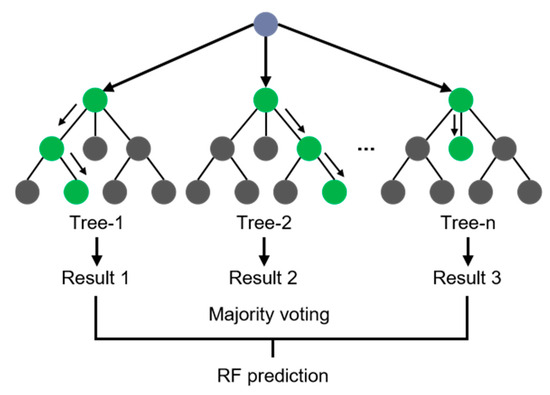
Figure 3. Schematic diagram of the RF ensemble learning principle.

For each task $\mathrm{k}\in \{\mathrm{1,2},3\}$, the residual at hour t is defined as:

$${\mathrm{e}}_{\mathrm{k},\mathrm{t}}={\mathrm{y}}_{\mathrm{k},\mathrm{t}}-{\widehat{\mathrm{y}}}_{\mathrm{k},\mathrm{t}}^{\mathrm{M}\mathrm{T}\mathrm{L}}$$

(23)

These residuals contain systematic deviations that typically exhibit short-term and episodic patterns. Although RF is not a recurrent model, combining the MTL-LSTM outputs with the RF input structure enables the tree-based model to effectively learn conditional residual dynamics.

To construct the RF input vector, the final RFECV-selected feature vector ${\tilde{\mathbf{x}}}_t$ is augmented with the preliminary predictions from the MTL-LSTM. The resulting input is expressed as

$${\mathrm{z}}_{\mathrm{t}}={\left[\begin{array}{cccc}{\tilde{\mathrm{x}}}_{\mathrm{t}}^{\mathrm{\top }},& {\widehat{\mathrm{y}}}_{1,\mathrm{t}}^{\mathrm{M}\mathrm{L}},& {\widehat{\mathrm{y}}}_{2,\mathrm{t}}^{\mathrm{M}\mathrm{T}\mathrm{L}},& {\widehat{\mathrm{y}}}_{3,\mathrm{t}}^{\mathrm{M}\mathrm{T}\mathrm{L}}\end{array}\right]}^{\mathrm{\top }}$$

(24)

which preserves essential information regarding exogenous conditions and embeds the long-term temporal dependencies extracted by the LSTM. This enriched input allows RF to capture localized residual structures that are conditioned on both environmental variables and the deep model’s internal temporal representation.

Given the input ${\mathrm{z}}_t$, a separate RF regressor is trained for each task k. Let ${\mathrm{f}}_{\mathrm{m},\mathrm{k}}(·)$ denote the prediction of the m-th regression tree in the ensemble, and let M be the total number of trees. The RF residual estimator is then defined as

$${\widehat{\mathrm{e}}}_{\mathrm{k},\mathrm{t}}={\displaystyle \frac{1}{\mathrm{M}}}\sum _{\mathrm{m}=1}^{\mathrm{M}}{\mathrm{f}}_{\mathrm{m},\mathrm{k}}\left({\mathrm{z}}_{\mathrm{t}}\right)$$

(25)

The final corrected prediction for each task is obtained by adding the estimated residual to the MTL-LSTM preliminary forecast:

$${\widehat{\mathrm{y}}}_{\mathrm{k},\mathrm{t}}^{\mathrm{f}\mathrm{i}\mathrm{n}\mathrm{a}\mathrm{l}}={\widehat{\mathrm{y}}}_{\mathrm{k},\mathrm{t}}^{\mathrm{M}\mathrm{T}\mathrm{L}}+{\widehat{\mathrm{e}}}_{\mathrm{k},\mathrm{t}}$$

(26)

This residual correction mechanism allows the RF to capture nonlinear residual structures that are not fully characterized by the deep learning model, thus improving the final prediction accuracy. By combining the temporal feature learning capability of the MTL-LSTM with the ensemble-based nonlinear modeling strength of the RF, the hybrid MTL-LSTM-RF model achieves robust and high-precision multi-energy loads forecasting under IES operating conditions.

3. Experimental Design and Data Processing

3.1. Data Sources and Preprocessing

This study used a complete historical operational dataset from a typical PIES located in eastern China for the full year of 2021. The dataset comprises three types of energy loads—electricity, cooling, and heating—recorded by the park’s Building Energy Management System, along with the corresponding meteorological variables obtained from the local meteorological monitoring station of the industrial park. All data were collected at hourly intervals, resulting in 8760 valid samples representing a full year of load variations. To facilitate model training and evaluation, the dataset was divided into training, validation, and testing sets in an 8:1:1 ratio.

To ensure the quality of the model input data, anomalies and missing values were first detected using the Interquartile Range (IQR) method. A time-context-aware mean imputation strategy was subsequently employed to correct them, which aims to maximally preserve the inherent temporal patterns of the load data. For a missing or anomalous value ${\mathrm{x}}_{\mathrm{t}}$ at time t, the imputed value is calculated as

$${\mathrm{x}}_{\mathrm{t}}={\displaystyle \frac{1}{\mathrm{N}}}\sum _{\mathrm{i}=1}^{\mathrm{N}}{\mathrm{x}}_{\mathrm{t}-24\mathrm{i}}$$

(27)

To eliminate scale differences among heterogeneous variables and stabilize the optimization of the MTL-LSTM, all numerical features involved in sequence modeling were standardized before training. A Z-score normalization was applied to the input sequences using the mean and standard deviation calculated exclusively from the training set, and the same scaling parameters were subsequently used to normalize the validation and test sets. This prevents information leakage and ensures consistent feature scaling across all experimental stages. The normalized inputs serve as the basis for constructing the multivariate time-series sequences fed into the MTL-LSTM.

3.2. Input Feature Construction and Selection

To explore the complex relationships between cooling, heating, and electricity loads and their external driving factors within the IES, this study conducted a quantitative analysis using Spearman’s rank correlation coefficient (SRCC). The results, presented in Figure 4, reveal that temperature exhibits a strong positive correlation with cooling (0.90) and electricity (0.62) loads, but a negative correlation with the heating load (−0.84). This indicates that cooling and electricity demands tend to increase with higher temperatures, while heating demand decreases. Humidity and wind speed, however, show weak correlations, suggesting that they exert only marginal influences on the loads during specific periods. Humidity and wind speed generally show weak correlations, exerting only marginal influences on the loads during specific periods. Regarding load couplings, electricity and cooling loads are highly positively correlated (0.74), reflecting the direct impact of electric-driven cooling systems on electricity consumption. Conversely, cooling-heating and electricity-heating pairs are generally negatively correlated, indicating the dynamic balance and trade-offs between energy conversion paths in a combined cooling and heating supply context.

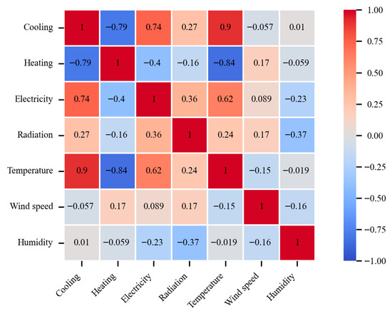
Figure 4. Correlation analysis between IES loads and meteorological factors.

Based on the correlation analysis and the operational characteristics of PIES, a comprehensive feature construction and selection strategy was formulated. The preliminary feature set was systematically constructed from three principal dimensions: temporal attributes, meteorological parameters, and multi-energy loads profiles. The constructed feature set contains D = 84 input features, as summarized in Table 1. Temporal attributes consisted of hour of day, day of week, and week index, which were cyclically encoded (sine–cosine) to represent daily and weekly regularities in energy-use patterns. Load-related features were built from historical cooling, heating, and electricity loads, with short-term lags from t−1 to t−24 and a weekly lag at t−168 for each load, yielding 25 autoregressive terms per load to capture system inertia and cross-energy coupling. Meteorological variables included air temperature, relative humidity, solar radiation, and wind speed. To account for the delayed response of loads to thermal conditions, air temperature was represented by three lagged values (t−1, t−3, t−6), reflecting the cumulative influence of recent temperature history on current demand. In contrast, humidity, radiation, and wind speed were introduced using their most recent value (t−1), which is sufficient to describe their immediate impact on the loads.

Table 1. Overview of the Constructed Input Features and Their Lag Structures.

Feature	Type	Lag	Number of Lags
Hour/Day/Week	Temporal	data	3
Cooling Load	Load-related	t-1 to t-24, t-168	25
Heating Load		t-1 to t-24, t-168	25
Electricity Load		t-1 to t-24, t-168	25
Temperature	Meteorological	t-1, t-3, t-6	3
Humidity		t-1	1
Radiation		t-1	1
Wind Speed		t-1	1
Total	-	-	84

Guided by expert knowledge of IES energy flow mechanisms, several physically meaningful features were retained before applying RFECV to ensure that features known to exert essential physical influences were not removed during recursive elimination. These expert-retained features include the temporal descriptors (hour, day of week, and week index), which capture the intrinsic daily and weekly periodicity of commercial energy-use behaviors; the lagged air-temperature features at t−1, t−3, and t−6, identified by the SRCC results as the dominant meteorological drivers and representing both immediate and accumulated thermal effects; and the key autoregressive load features at lags t−1 and t−24 for cooling, heating, and electricity, which describe short-term inertia and strong daily recurrence associated with building thermal characteristics and equipment operating cycles. Preserving these features enhances interpretability and maintains consistency with the known thermodynamic and operational behavior of PIES. After fixing these expert-retained features, the remaining features were evaluated using RFECV with a five-fold TimeSeriesSplit. A value of K = 5 was adopted because it provides a widely used balance between temporal coverage and validation stability for time-series forecasting while preserving the chronological structure of the load data, ensuring that each fold contains sufficient consecutive observations for reliable training and evaluation.

The RFECV process iteratively removed the least contributing variables, with the final subset determined by the highest cross-validation score. Figure 5a–c present the importance ranking of the autoregressive lag terms. The cooling load is dominated by recent lags, with cooling-t−1 having a weight far exceeding others, while t−2 and t−3 still contribute significantly, reflecting the short-term inertia and rapid response of the cooling load. The heating load shows a bimodal importance at heating-t−1 and t−23, indicating its dependence on both the immediate previous state and the corresponding period from the previous day, consistent with the thermal storage effect of buildings and the time delay in pipeline transmission. The electricity load is dominated by electricity-t−24, demonstrating the strongest daily periodicity, which aligns with production schedules and the rhythmic operation of electric-driven equipment.

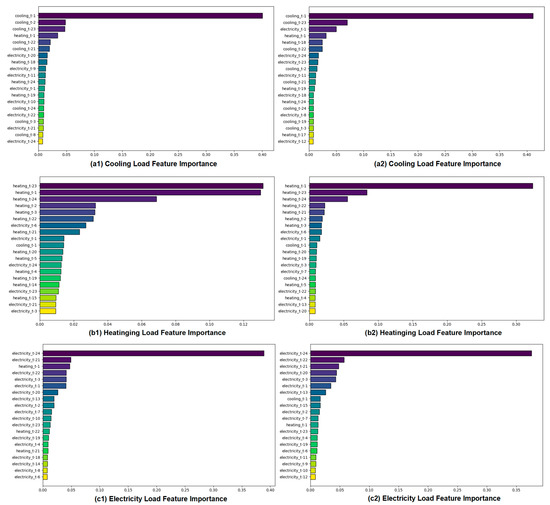
Figure 5. Importance ranking of preliminary input features for cooling, heating, and electricity loads under different operating conditions.

Furthermore, it is noteworthy that the feature rankings from RFECV are not solely dominated by a load’s own autoregressive terms. Lagged terms from other energy flows also exhibit non-negligible importance. For instance, in cooling load prediction, heating-t−1 and electricity-t−2 retain considerable weights, suggesting that short-term variations in heating and electricity loads influence the transient response of the cooling system, consistent with the energy flow interactions in a combined cooling and heating system. In heating load prediction, the importance of cooling-t−2 and electricity-t−3 increases, reflecting the indirect feedback of chiller operation on waste heat recovery and the thermal network dynamics. For electricity load prediction, several lagged terms from cooling and heating loads also enter the feature subset, revealing that electricity consumption not only reflects the periodicity of user behavior but is also co-modulated by the operational characteristics of cooling and heating equipment.

These results demonstrate that RFECV not only identifies the dominant autoregressive drivers for each load but also uncovers meaningful cross-load lag dependencies that reflect the intrinsic coupling mechanisms within the system. More importantly, the comparison of feature-importance rankings under two representative operating conditions reveals that the selection pattern exhibits both stability and adaptiveness. Core autoregressive features (e.g., cooling_t−1, heating_t−1, electricity_t−24) consistently remain the most influential across conditions, highlighting the robustness of the feature-selection process. At the same time, notable shifts in the rankings of secondary cross-load features—such as cooling–heating and heating–electricity lag terms—indicate that RFECV can dynamically adjust to changes in thermal–electric interaction intensity caused by varying weather, equipment scheduling, or seasonal operating modes. This combination of stability in the primary drivers and adaptive adjustment of secondary features provides strong evidence that the RFECV procedure does not overfit to any single operating state but instead yields feature subsets that remain physically meaningful and predictive across diverse system conditions. Consequently, the selected features offer reliable and informative inputs for the shared representation layer in the subsequent MTL framework, further supporting accurate modeling of multi-energy coupling behaviors.

3.3. Evaluation Metrics

To quantitatively assess the forecasting performance of the proposed MTL-LSTM-RF model and its counterparts, this study employs four widely used evaluation metrics: the Root Mean Square Error (RMSE), Mean Absolute Error (MAE), Mean Absolute Percentage Error (MAPE), and the coefficient of determination (R²). These metrics jointly characterize different aspects of prediction accuracy by measuring absolute deviation, squared deviation, relative deviation, and goodness-of-fit between the predicted and true load values. The metrics are formally defined as follows

$$\mathrm{R}\mathrm{M}\mathrm{S}\mathrm{E}=\sqrt{{\displaystyle \frac{1}{{\mathrm{N}}_{\mathrm{t}\mathrm{e}}}}\sum _{\mathrm{t}\in {\mathsf{\Omega }}_{\mathrm{t}\mathrm{e}}}({\mathrm{y}}_{\mathrm{k},\mathrm{t}}-{\widehat{\mathrm{y}}}_{\mathrm{k},\mathrm{t}}{)}^2}$$

(28)

$$\mathrm{M}\mathrm{A}\mathrm{E}={\displaystyle \frac{1}{{\mathrm{N}}_{\mathrm{t}\mathrm{e}}}}\sum _{\mathrm{t}\in {\mathsf{\Omega }}_{\mathrm{t}\mathrm{e}}}|{\mathrm{y}}_{\mathrm{k},\mathrm{t}}-{\widehat{\mathrm{y}}}_{\mathrm{k},\mathrm{t}}|$$

(29)

$$\mathrm{M}\mathrm{A}\mathrm{P}\mathrm{E}={\displaystyle \frac{1}{N_{\mathrm{t}\mathrm{e}}}}\sum _{\mathrm{t}\in {\mathsf{\Omega }}_{\mathrm{t}\mathrm{e}}}\left|{\displaystyle \frac{{\mathrm{y}}_{\mathrm{k},\mathrm{t}}-{\mathrm{y}}_{\mathrm{k},\mathrm{t}}}{{\mathrm{y}}_{\mathrm{k},\mathrm{t}}}}\right|\times 100\mathrm{\%}$$

(30)

$${\mathrm{R}}^2=1-{\displaystyle \frac{\sum _{\mathrm{t}\in {\mathsf{\Omega }}_{\mathrm{v}}}({\mathrm{y}}_{\mathrm{k},\mathrm{t}}-{\widehat{\mathrm{y}}}_{\mathrm{k},\mathrm{t}}{)}^2}{\sum _{\mathrm{t}\in {\mathsf{\Omega }}_{\mathrm{e}}}({\mathrm{y}}_{\mathrm{k},\mathrm{t}}-{\overline{\mathrm{y}}}_{\mathrm{k}}{)}^2}}$$

(31)

4. Results and Discussion

4.1. Hyperparameter Configuration

To thoroughly validate the performance of the proposed hybrid model, this section details the hyperparameter configurations for the developed model and all baseline models. All experiments were conducted under identical hardware and software environments to ensure the comparability of the results.

The MTL-LSTM model was implemented to forecast cooling, heating, and electricity loads using a sliding input window of 24 time steps, enabling the extraction of daily cyclical patterns and short-term temporal dependencies. The shared temporal encoder consisted of two stacked LSTM layers, each with 128 hidden units, followed by a dropout layer with a rate of 0.2 applied before the task-specific output heads. The model was trained using the Adam optimizer with an initial learning rate of 0.001, a batch size of 64, and a maximum of 200 epochs. A dynamic task-weighting mechanism was employed, allowing the relative importance of the three forecasting tasks to be adaptively adjusted throughout the training process.

Training stability and generalization were further enhanced through a collection of regularization and optimization strategies. Gradient clipping was applied to the recurrent layers with a maximum norm of 5 to avoid exploding gradients. An adaptive learning-rate scheduler (ReduceLROnPlateau) was used with a patience of 10 epochs to refine the optimization process when validation loss improvements slowed. Early stopping was employed to terminate training when validation performance failed to improve for 20 consecutive epochs, thereby preventing overfitting. In addition, L2 weight decay with a coefficient of 0.0001 was incorporated into the Adam optimizer to constrain model complexity.

For the second-stage residual correction, an individual RF model was trained for each energy loads. The RF models used the RFECV-selected feature subsets concatenated with the preliminary MTL-LSTM forecasts to learn the residual patterns that the deep network did not fully capture. The primary RF hyperparameters—including the number of trees, maximum depth, and minimum samples per leaf—were determined through grid search combined with a rolling time-series cross-validation procedure. This residual-learning configuration enables the RF to model localized fluctuations and non-stationary behaviors present in the residual sequences.

All experiments were conducted on a personal workstation equipped with a 12th Gen Intel Core i5-12600KF CPU (3.70 GHz), 16 GB of RAM, and an NVIDIA GeForce RTX 4060 Ti GPU with 8 GB of dedicated memory. The implementation was developed in Python 3.9.10, with the deep learning components built using PyTorch 2.0.1 and the RF models implemented via scikit-learn 1.6.1. This hardware–software configuration ensures stable computational performance and reproducibility across all experiments.

4.2. Experimental Results

To comprehensively evaluate the performance of the proposed hybrid RFECV + MTL-LSTM-RF model in park-level energy station load forecasting, a comparative analysis was conducted against four benchmark models: RFECV + MTL-LSTM, Pearson-Correlation-Filtered MTL-LSTM (Pearson + MTL-LSTM), MTL-LSTM, and the conventional LSTM. All models were trained and tested on identical datasets, using the same input features, normalization procedures, and hyperparameter configurations to ensure fair comparability.

Table 2 summarizes the forecasting performance of all models in terms of MAPE, RMSE, and MAE for cooling, heating, and electricity loads. The results demonstrate that the proposed RFECV + MTL-LSTM-RF model consistently outperforms the other approaches across all three load types. Specifically, the multi-task shared-representation structure of the MTL-LSTM model yields markedly better accuracy than the single-task LSTM, confirming that inter-task knowledge transfer effectively enhances forecasting precision. With the incorporation of Pearson-correlation-based feature filtering, the Pearson + MTL-LSTM model achieves further reduction in prediction errors, indicating that removing linearly redundant variables helps lower noise in the input space and improves model expressiveness. When the RFECV feature-selection mechanism is introduced, redundant variables are removed and the input dimensionality is optimized, thereby reducing noise interference caused by irrelevant features. Consequently, the RMSE values for cooling, heating, and electricity loads decrease to 1.428 GJ/h, 2.374 GJ/h, and 1.934 kW, respectively. Finally, by incorporating the RF-based residual-correction module, the forecasting errors are further mitigated, with the RMSE reduced to 1.159 GJ/h, 2.081 GJ/h, and 1.641 kW for the three loads, respectively. These results validate the effectiveness of the model’s modular and staged design.

Table 2. Performance comparison of different models.

Model	MAPE (%)			RMSE			MAE			R2
	Cooling GJ/h	Heating GJ/h	Electric kW	Cooling GJ/h	Heating GJ/h	Electric kW	Cooling GJ/h	Heating GJ/h	Electric kW	Cooling GJ/h	Heating GJ/h	Electric kW
LSTM	7.38	5.11	5.76	1.859	3.357	2.809	1.531	2.942	2.397	0.875	0.868	0.877
MTL-LSTM	6.17	3.89	3.97	1.519	2.636	1.991	1.281	2.228	1.651	0.894	0.887	0.869
Pearson + MTL-LSTM	5.92	3.42	3.91	1.475	2.462	1.964	1.229	1.949	1.612	0.904	0.891	0.908
RFECV + MTL-LSTM	5.69	3.28	3.79	1.428	2.374	1.934	1.175	1.862	1.563	0.916	0.903	0.918
RFECV + MTL-LSTM-RF	4.65	2.79	3.01	1.159	2.081	1.641	0.945	1.587	1.264	0.932	0.926	0.936

To further improve the reliability of the evaluation, a nonparametric bootstrap procedure with 1000 resampling iterations was used to estimate the 95% confidence intervals (CIs) of MAPE, RMSE, and MAE for each model. The results show that the RFECV + MTL-LSTM-RF model consistently produces narrower intervals compared with the other models. For example, its cooling-load RMSE CI lies between approximately 1.13 and 1.20 GJ/h, which is clearly tighter than that of the Pearson + MTL-LSTM model (about 1.39–1.48 GJ/h) and much narrower than that of the baseline MTL-LSTM (around 1.57–1.65 GJ/h). Similar patterns of CI contraction are also observed for the heating and electricity loads. These findings indicate that the improvements of the proposed hybrid framework are statistically robust rather than a result of sampling variability.

Figure 6 illustrates the comparison between predicted and actual values for the three energy loads across a representative week. As shown in the figure, the MTL-LSTM model provides a basic level of fit, while the Pearson + MTL-LSTM variant achieves visibly closer alignment with the actual profiles by improving the tracking of peak–valley patterns and local fluctuations. After applying RFECV-based feature refinement, the RFECV + MTL-LSTM model further suppresses noise-induced oscillations and enhances the smoothness and stability of the predicted curves. With the addition of RF-based residual correction, the final RFECV + MTL-LSTM-RF model attains the closest match to the measured loads—particularly during periods of intensive fluctuations and peak demand—where the amplitude of prediction deviation is significantly reduced.

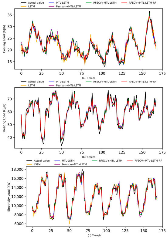
Figure 6. Comparison between predicted and actual values for cooling, heating, and electricity loads. (a) Cooling load; (b) Heating load; (c) Electricity load.

To further confirm that the performance improvement stems from a genuine enhancement in distributional accuracy—rather than spurious fits at isolated points—Figure 7 presents the daily prediction curves together with the corresponding box-plot distributions of relative errors. In the typical daily load profile, the Pearson + MTL-LSTM model already exhibits visibly better alignment with the actual load trajectory, reducing local biases and capturing peak–valley transitions more accurately. The RFECV + MTL-LSTM model further narrows the deviation band and mitigates short-term overshooting or undershooting, indicating that feature refinement contributes to more stable temporal behavior. Building on these advantages, the RFECV + MTL-LSTM-RF model delivers the closest overall fit to the true load profile throughout the day, with the smallest discrepancies during periods of rapid load variation. The box plots reveal the same progressive improvement. Compared with Pearson + MTL-LSTM, the RFECV + MTL-LSTM model exhibits a noticeably reduced interquartile range (IQR) and shorter whiskers, reflecting contractions in both central dispersion and tail variability. On this basis, the RFECV + MTL-LSTM-RF model achieves the smallest IQR, the shortest whiskers, and the fewest extreme deviations among the three models. Quantitatively, the average relative errors for cooling, heating, and electricity loads decrease from 0.0535, 0.0329, and 0.0433 under Pearson + MTL-LSTM to 0.0503, 0.0299, and 0.0378 under RFECV + MTL-LSTM, and are further reduced to 0.0329, 0.0250, and 0.0279 with RFECV + MTL-LSTM-RF. This contraction in both error magnitude and variance indicates that prediction uncertainty is effectively suppressed, confirming that the model yields more stable and reliable results overall. These findings demonstrate that the residual-correction layer not only mitigates random fluctuations and upper-tail deviations but also achieves a bidirectional optimization of the error distribution, reinforcing the robustness of the final hybrid model.

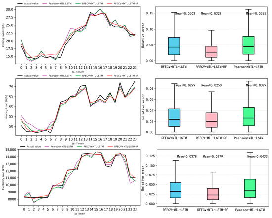
Figure 7. Forecasting performance and error distribution before and after residual correction on a typical day. (a) Cooling load; (b) Heating load; (c) Electricity load.

To further examine the model’s generalization capability and stability, residual scatter analysis was performed for all forecasting tasks, as shown in Figure 8a–c. In these plots, the horizontal axis represents the predicted values, the vertical axis denotes the residuals, and the standard deviation (σ) is introduced to quantify residual dispersion. Among the baseline models, the Pearson + MTL-LSTM variant already produces slightly more compact and less biased residual clouds than the original MTL-LSTM, reflecting the benefits of removing linearly redundant features. The RFECV + MTL-LSTM model further reduces tail fluctuation and attenuates large-magnitude deviations, suggesting that feature refinement contributes to more stable error behavior. The RFECV + MTL-LSTM-RF model exhibits the most concentrated and symmetric residual distribution around zero, markedly outperforming the baseline models. Its residual points cluster densely near the horizontal axis with visibly fewer extreme departures, indicating consistently lower prediction uncertainty across the entire range of load conditions. Numerically, the residual standard deviations for cooling, heating, and electricity loads are 1 GJ/h, 1.83 GJ/h, and 445.05 kW, respectively—approximately 30% lower on average than those of the Pearson + MTL-LSTM and RFECV + MTL-LSTM models. This hierarchical reduction in σ—from MTL-LSTM to Pearson + MTL-LSTM, then to RFECV + MTL-LSTM, and finally to RFECV + MTL-LSTM-RF—demonstrates the stepwise effectiveness of correlation-based filtering, feature refinement, and residual correction. This confirms that the residual correction module effectively enhances forecasting stability and generalization across varying load magnitudes and operating conditions.

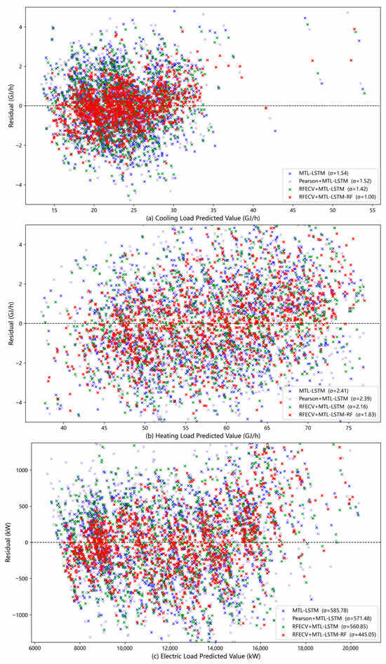
Figure 8. Residual scatter distributions of different models for cooling, heating, and electricity loads.

The above results systematically verify the superiority of the proposed framework from the perspectives of forecasting accuracy, residual-distribution characteristics, and generalization performance. Nevertheless, the computational efficiency of the model is equally critical for evaluating its suitability in engineering applications, as practical deployment requires not only accurate predictions but also manageable offline computation and sufficiently fast online forecasting. Assessing these aspects helps to clarify whether the proposed multi-stage architecture can operate effectively within real IES scheduling environments. Table 3 summarizes the time consumption of each model across the feature-selection, training, residual-correction, and single-step forecasting stages.

Table 3. Comparison of Training Cost and Forecasting Efficiency Across Different Models.

Model	Feature Selection Time (s)	Training Time (s)	RF Correction Time (s)	Total Offline Cost (s)	Forecasting Time (s)
LSTM	-	327.28	-	327.28	0.2352
MTL-LSTM	-	176.35	-	176.35	0.0913
Pearson + MTL-LSTM	2	168.73	-	170.73	0.0852
RFECV + MTL-LSTM	267.82	158.83	-	426.65	0.0822
RFECV + MTL-LSTM-RF	267.82	158.83	13.57	440.22	0.0868

The conventional single-task LSTM requires independent training for cooling, heating, and electricity loads, whereas the MTL-LSTM jointly learns all three tasks within a unified temporal representation. This shared-learning mechanism substantially reduces redundant feature extraction and yields a baseline training time of 176.35 s for the multi-task model. Incorporating Pearson-based filtering further decreases the input dimensionality and shortens the training time by approximately 4% relative to the MTL-LSTM baseline, reflecting the benefit of removing linearly redundant predictors and stabilizing the subsequent learning process. RFECV, in turn, provides a more comprehensive feature-refinement mechanism by iteratively eliminating weakly relevant variables under a cross-validation scheme. This procedure reduces the effective feature space before multi-task learning and contributes to improved model conditioning. Although RFECV requires 267.82 s for feature selection and increases the total offline cost relative to the MTL baseline, the RFECV-enhanced hybrid models deliver notable gains in forecasting accuracy and exhibit consistently improved residual stability, as evidenced in Table 2. These performance improvements provide a clear justification for the additional offline computation. Moreover, the RFECV + MTL-LSTM-RF model maintains a forecasting latency that is slightly faster than that of the MTL-LSTM baseline, indicating that the enhanced model retains efficient inference capability despite its more elaborate training pipeline.

Taken as a whole, the analyses of forecasting accuracy, residual-distribution characteristics, and computational efficiency presented in this section consistently demonstrate that the proposed hybrid framework delivers reliable predictive performance across all load types while maintaining stable error behavior under both typical and volatile conditions. These results underscore the universality and robustness of the multi-layer integrated architecture, indicating that the gains in accuracy and stability are achieved with a computational cost that remains acceptable for practical IES applications. Building on these empirical findings, the following discussion further examines the underlying mechanisms that contribute to the effectiveness of the proposed approach.

4.3. Discussion

The experimental results provide several insights into the mechanisms underlying the performance of the proposed hybrid RFECV + MTL-LSTM-RF framework. The multi-task architecture enables the model to leverage shared temporal patterns among cooling, heating, and electricity loads, which often respond jointly to weather and operational conditions. This shared representation helps the model capture synchronized fluctuations that single-task approaches tend to miss.

The RFECV-based feature refinement further stabilizes the forecasting process by removing redundant or weakly relevant features, thereby reducing noise transmission into the learning pipeline. This effect is particularly evident when comparing Pearson + MTL-LSTM with RFECV-enhanced models, suggesting that systematic data-driven feature screening provides more consistent benefits than simple correlation-based filtering alone. Additionally, the RF residual-correction layer effectively addresses nonlinear and heteroscedastic components of forecasting errors, yielding more compact residual distributions and improving robustness during periods of rapid load variation.

These observations also have implications for sustainable IES. As the proportion of renewable resources such as photovoltaics and wind power continues to grow, reliable short-term load forecasting becomes increasingly important for maintaining operational stability and supporting flexible scheduling. The modular structure of the proposed framework makes it well suited for future extension toward multi-energy prediction and renewable-integration scenarios.

While the proposed framework demonstrates strong predictive capability, it still operates as an open-loop forecasting model under assumed system conditions and does not explicitly account for the physical and economic constraints inherent to real IES operation. Physically, equipment capacity limits, ramping capabilities, and dynamic response characteristics define the feasible region of short-term load variations, meaning that actual loads cannot freely follow weather-driven signals or historical inertia. Economically, time-of-use tariffs, demand-response incentives, and renewable-driven dispatch adjustments reshape load profiles through price- and cost-driven behavioral changes. Incorporating such physical and economic constraints into future forecasting frameworks would shift the task from predicting the most likely load trajectory to generating feasible trajectories that reflect both operational limitations and market-responsive behavior.

Nonetheless, the discussion should acknowledge that the model has not yet incorporated renewable generation dynamics, energy storage behavior, or cross-site validation. These aspects are essential for fully supporting next-generation sustainable energy station operation and represent important directions for future work.

Looking forward, future integration of renewable energy forecasting will enable the proposed framework to operate in a more unified multi-energy setting. In such scenarios, RFECV can be extended to simultaneously select informative predictors for both load-side and generation-side variables—for example, irradiance-, cloud-cover-, and temperature-related features for PV generation, and wind-speed-, turbulence-, and direction-related features for wind power. This unified feature-selection process would allow the model to identify cross-dependencies not only among cooling, heating, and electricity loads, but also between loads and renewable outputs. Likewise, embedding renewable generation forecasting tasks into the MTL-LSTM architecture would allow the shared temporal encoder to learn broader multi-energy interactions, capturing correlations such as load–PV coupling under high-irradiance conditions or wind–electricity complementarity during rapid weather changes. Such an extension would further enhance the framework’s applicability to renewable-rich IES and support integrated forecasting and scheduling needs in future sustainable energy stations.

5. Conclusions

This study presents a hybrid RFECV + MTL-LSTM-RF forecasting framework for cooling, heating, and electricity loads in park-level energy stations. By integrating multi-task temporal representation learning, data-driven feature refinement, and residual-based error correction, the proposed framework achieves significant and consistent accuracy improvements over benchmark models. The hybrid approach benefits from the complementary strengths of its components: shared representations across correlated energy loads, optimized and noise-reduced feature inputs, and an additional correction layer capable of capturing complex residual structures, while the overall computational cost of the hybrid architecture remains acceptable and its forecasting latency stays well within the sub-second range, supporting real-time applicability in practical IES operations.

Methodologically, the work contributes a structured and interpretable modeling pipeline, in which feature selection, sequence prediction, and residual learning are tightly coupled. The RFECV procedure effectively removes redundant meteorological and operational variables, thereby enhancing learning stability. The MTL-LSTM architecture exploits cross-load dependencies to better capture joint fluctuations and common temporal patterns. Finally, the RF-based residual module addresses nonlinear and heteroscedastic error components that conventional neural networks may overlook, leading to improved distributional fidelity and reduced extreme deviations.

Beyond its methodological contributions, the proposed framework holds practical value for sustainable IES. Accurate short-term load prediction supports refined scheduling, reduced auxiliary energy consumption, and improved utilization of distributed resources. As renewable energy penetration continues to increase—particularly photovoltaics and wind power—the hybrid architecture offers a scalable basis for integrating renewable generation forecasting and multi-energy coordination. The enhanced robustness and reduced uncertainty achieved by the framework contribute directly to the efficient and low-carbon operation of modern park-level energy stations.

Several limitations should be acknowledged. The analysis is based on data from a single energy station, and broader validation across multiple sites with diverse climatic and operational conditions is needed. The current framework focuses solely on load-side forecasting and does not incorporate renewable outputs, energy storage behavior, or cross-site generalization. Moreover, physical constraints—such as equipment capacity limits, ramping capabilities, and dynamic response characteristics—and economic dispatch factors, including time-of-use pricing and demand-response incentives, were not explicitly modeled. Future work will extend the framework toward holistic multi-energy forecasting by integrating renewable generation prediction and storage dynamics. Such an extension would enable RFECV to conduct unified feature selection over both load-side and generation-side variables, while allowing the MTL-LSTM architecture to learn broader cross-energy dependencies. Together, these developments will further enhance the practicality and scalability of the proposed method for real-world sustainable and resilient energy systems.

References

- Mado, I.; Rajagukguk, A.; Triwiyatno, A.; Fadllullah, A. Short-term electricity load forecasting model based dsarima. Int. J. Electr. Energy Power Syst. Eng. 2022, 5, 6–11. [Google Scholar] [CrossRef]
- Pełka, P. Analysis and forecasting of monthly electricity demand time series using pattern-based statistical methods. Energies 2023, 16, 827. [Google Scholar] [CrossRef]
- Luo, H.; Tong, C.; Gu, W.; Li, Z. Time-Series Imaging for Improving the Accuracy of Short-Term Load Forecasting. Energy 2025, 333, 137282. [Google Scholar] [CrossRef]
- Li, X.; Jiang, M.; Cai, D.; Song, W. A hybrid forecasting model for electricity demand in sustainable power systems based on Support Vector Machine. Energies 2024, 17, 4377. [Google Scholar] [CrossRef]
- Dakheel, F.; Çevik, M. Optimizing Smart Grid Load Forecasting via a Hybrid LSTM-XGBoost Framework: Enhancing Accuracy, Robustness, and Energy Management. Energies 2025, 18, 2842. [Google Scholar] [CrossRef]
- Liu, H. The forecast of household power load based on genetic algorithm optimizing BP neural network. J. Phys. Conf. Ser. 2021, 1871, 12110. [Google Scholar] [CrossRef]
- Yang, M.; Liu, D.; Su, X.; Wang, J.; Cui, Y. Ultra-short-term load prediction of integrated energy system based on load similar fluctuation set classification. Front. Energy Res. 2023, 10, 1037874. [Google Scholar] [CrossRef]
- Wu, L.; Kong, C.; Hao, X.; Chen, W. A short-term load forecasting method based on GRU-CNN hybrid neural network model. Math. Probl. Eng. 2020, 2020, 1428104. [Google Scholar] [CrossRef]
- Guo, X.; Zhao, Q.; Zheng, D.; Ning, Y.; Gao, Y. A short-term load forecasting model of multi-scale CNN-LSTM hybrid neural network considering the real-time electricity price. Energy Rep. 2020, 6, 1046–1053. [Google Scholar] [CrossRef]
- Chiu, M.C.; Hsu, H.W.; Chen, K.S.; Wen, C.Y. A hybrid CNN-GRU based probabilistic model for load forecasting from individual household to commercial building. Energy Rep. 2023, 9, 94–105. [Google Scholar] [CrossRef]
- Peng, L.L.; Fan, G.F.; Yu, M.; Chang, Y.C.; Hong, W.C. Electric load forecasting based on wavelet transform and random forest. Adv. Theory Simul. 2021, 4, 2100334. [Google Scholar] [CrossRef]
- Li, K.; Huang, W.; Hu, G.; Li, J. Ultra-short term power load forecasting based on CEEMDAN-SE and LSTM neural network. Energy Build. 2023, 279, 112666. [Google Scholar] [CrossRef]
- Wan, A.; Chang, Q.; Khalil, A.L.B.; He, J. Short-term power load forecasting for combined heat and power using CNN-LSTM enhanced by attention mechanism. Energy 2023, 282, 128274. [Google Scholar] [CrossRef]
- Liu, H.; Li, H.J.; Liu, Y.W.; Zou, Q. Power load forecasting method based on VMD and GWO-SVR. Mod. Electron. Technol. 2020, 43, 175–180. [Google Scholar]
- Ouyang, T.; Huang, H.; He, Y.; Tang, Z. Chaotic wind power time series prediction via switching data-driven modes. Renew. Energy 2020, 145, 270–281. [Google Scholar] [CrossRef]
- Dudek, G. A comprehensive study of random forest for short-term load forecasting. Energies 2022, 15, 7547. [Google Scholar] [CrossRef]
- Haq, I.U.; Khalid, M.; Manzoor, U. A comparative analysis of deep learning models for short-term load forecasting. In Proceedings of the 2023 IEEE 19th International Conference on Automation Science and Engineering (CASE), Auckland, New Zealand, 26–30 August 2023; IEEE: Piscataway, NJ, USA, 2023; pp. 1–7. [Google Scholar]
- Zhang, L.; Shi, J.; Wang, L.; Xu, C. Electricity, heat, and gas load forecasting based on deep multitask learning in industrial-park integrated energy system. Entropy 2020, 22, 1355. [Google Scholar] [CrossRef] [PubMed]
- Niu, D.; Yu, M.; Sun, L.; Gao, T.; Wang, K. Short-term multi-energy load forecasting for integrated energy systems based on CNN-BiGRU optimized by attention mechanism. Appl. Energy 2022, 313, 118801. [Google Scholar] [CrossRef]
- Xuan, W.; Shouxiang, W.; Qianyu, Z.; Shaomin, W.; Liwei, F. A multi-energy load prediction model based on deep multi-task learning and ensemble approach for regional integrated energy systems. Int. J. Electr. Power Energy Syst. 2021, 126, 106583. [Google Scholar] [CrossRef]
- Tang, Y.; Yang, K.; Zhang, S.; Zhang, Z. Wind power forecasting: A hybrid forecasting model and multi-task learning-based framework. Energy 2023, 278, 127864. [Google Scholar] [CrossRef]
- Sun, Q.; Wang, X.; Zhang, Y.; Zhang, F.; Zhang, P.; Gao, W. Multiple load prediction of integrated energy system based on long short-term memory and multi-task learning. Autom. Electr. Power Syst. 2021, 45, 63–70. [Google Scholar]
- Tan, Z.; De, G.; Li, M.; Lin, H.; Yang, S.; Huang, L.; Tan, Q. Combined electricity-heat-cooling-gas load forecasting model for integrated energy system based on multi-task learning and least square support vector machine. J. Clean. Prod. 2020, 248, 119252. [Google Scholar] [CrossRef]
- Su, Z.; Zheng, G.; Hu, M.; Kong, L.; Wang, G. Short-term load forecasting of regional integrated energy system based on spatio-temporal convolutional graph neural network. Electr. Power Syst. Res. 2024, 232, 110427. [Google Scholar] [CrossRef]
- Zhang, Q.; Chen, J.; Xiao, G.; He, S.; Deng, K. TransformGraph: A novel short-term electricity net load forecasting model. Energy Rep. 2023, 9, 2705–2717. [Google Scholar] [CrossRef]
- Harikrishnan, G.R.; Sreedharan, S. Advanced short-term load forecasting for residential demand response: An XGBoost-ANN ensemble approach. Electr. Power Syst. Res. 2025, 242, 111476. [Google Scholar]
- Liao, W.; Bak-Jensen, B.; Pillai, J.R.; Yang, Z.; Liu, K. Short-term power prediction for renewable energy using hybrid graph convolutional network and long short-term memory approach. Electr. Power Syst. Res. 2022, 211, 108614. [Google Scholar] [CrossRef]
- Kavaliauskas, Ž.; Milieška, M.; Blažiūnas, G.; Gecevičius, G.; Zhairabany, H. Neural network approaches for generation forecasting and conceptual design in hybrid renewable energy systems. Int. J. Electr. Power Energy Syst. 2025, 172, 111241. [Google Scholar] [CrossRef]
- Xie, M.; Lin, S.; Dong, K.; Zhang, S. Short-Term Prediction of Multi-Energy Loads Based on Copula Correlation Analysis and Model Fusions. Entropy 2023, 25, 1343. [Google Scholar] [CrossRef] [PubMed]
- Sun, F.; Huo, Y.; Fu, L.; Liu, H.; Wang, X.; Ma, Y. Load-forecasting method for IES based on LSTM and dynamic similar days with multi-features. Glob. Energy Interconnect. 2023, 6, 285–296. [Google Scholar] [CrossRef]
- Jebli, I.; Belouadha, F.Z.; Kabbaj, M.I.; Tilioua, A. Prediction of solar energy guided by pearson correlation using machine learning. Energy 2021, 224, 120109. [Google Scholar] [CrossRef]
- Yu, J.; Li, X.; Yang, L.; Li, L.; Huang, Z.; Shen, K.; Yang, X.; Yang, X.; Xu, Z.; Zhang, D.; et al. Deep learning models for PV power forecasting. Energies 2024, 17, 3973. [Google Scholar] [CrossRef]
- Liu, Y.; Wang, J. Transfer learning based multi-layer extreme learning machine for probabilistic wind power forecasting. Appl. Energy 2022, 312, 118729. [Google Scholar] [CrossRef]
- Morgoeva, A.D.; Morgoev, I.D.; Klyuev, R.V.; Klyuev, R.V.; Kochkovskaya, S.S. Hourly electricity generation forecasting for a solar power plant using machine learning algorithms. Izvestiya Tomsk Polytechnic University. Geo Assets Eng. 2023, 334, 7–19. (In Russian) [Google Scholar] [CrossRef]
- Casanova, R.H.; Conde, A. Enhancement of LSTM models based on data pre-processing and optimization of Bayesian hyperparameters for day-ahead photovoltaic generation prediction. Comput. Electr. Eng. 2024, 116, 109162. [Google Scholar] [CrossRef]
- Bahij, Z.; Yan, B. A Multi-layer Weather Classification-based Regression Model for PV Power Prediction. In Proceedings of the 2024 IEEE 20th International Conference on Automation Science and Engineering (CASE), Bari, Italy, 28 August–1 September 2024; IEEE: Piscataway, NJ, USA, 2024; pp. 3231–3236. [Google Scholar]
- Cavus, M.; Allahham, A. Spatio-Temporal Attention-Based Deep Learning for Smart Grid Demand Prediction. Electronics 2025, 14, 2514. [Google Scholar] [CrossRef]
- Wang, S.; Wang, S.; Chen, H.; Gu, Q. Multi-energy load forecasting for regional integrated energy systems considering temporal dynamic and coupling characteristics. Energy 2020, 195, 116964. [Google Scholar] [CrossRef]
- Mirza, A.F.; Mansoor, M.; Usman, M.; Ling, Q. A comprehensive approach for PV wind forecasting by using a hyperparameter tuned GCVCNN-MRNN deep learning model. Energy 2023, 283, 129189. [Google Scholar] [CrossRef]
- Zhang, C.; Li, J.; Zhao, Y.; Li, T.; Chen, Q.; Zhang, X.; Qiu, W. Problem of data imbalance in building energy load prediction: Concept, influence, and solution. Appl. Energy 2021, 297, 117139. [Google Scholar] [CrossRef]
- Huang, N.; Ren, S.; Liu, J.; Cai, G.; Zhang, L. Multi-task learning and single-task learning joint multi-energy load forecasting of integrated energy systems considering meteorological variations. Expert Syst. Appl. 2025, 288, 128269. [Google Scholar] [CrossRef]
- Chen, H.; Zhu, M.; Hu, X.; Wang, J.; Sun, Y.; Yang, J.; Li, B.; Meng, X. Multifeature Short-Term Power Load Forecasting Based on GCN-LSTM. Int. Trans. Electr. Energy Syst. 2023, 2023, 8846554. [Google Scholar] [CrossRef]
- Chaibi, M.; Tarik, L.; Berrada, M.; El Hmaidi, A. Machine learning models based on random forest feature selection and Bayesian optimization for predicting daily global solar radiation. Int. J. Renew. Energy Dev. 2022, 11, 309. [Google Scholar] [CrossRef]
- Sikdar, S.; Hooker, G.; Kadiyali, V. Variable Importance Measures for Multivariate Random Forests. J. Data Sci. 2025, 23, 243–263. [Google Scholar] [CrossRef]
Disclaimer/Publisher’s Note: The statements, opinions and data contained in all publications are solely those of the individual author(s) and contributor(s) and not of MDPI and/or the editor(s). MDPI and/or the editor(s) disclaim responsibility for any injury to people or property resulting from any ideas, methods, instructions or products referred to in the content. |
© 2025 by the authors. Licensee MDPI, Basel, Switzerland. This article is an open access article distributed under the terms and conditions of the Creative Commons Attribution (CC BY) license (https://creativecommons.org/licenses/by/4.0/).