Bayesian–Kalman Fusion Framework for Thermal Fault Diagnosis of Battery Energy Storage Systems

Abstract

Fault diagnosis of battery energy storage systems (BESSs) in dynamic operating conditions presents significant challenges due to complex spatiotemporal patterns and measurement noise. This research proposes a novel thermal fault diagnosis framework for BESSs based on Bayesian inference and a Kalman filter. Firstly, PLS-based spatiotemporal feature extraction is designed to capture temporal dependencies. Based on Bayesian global exploration and Kalman real-time weight adaptation, a dual-stage optimization strategy is proposed to derive a multiscale detection index with the dominant statistic, the residual statistic, and the module voltage similarity. A time window-based cumulative contribution strategy is constructed for precise cell localization. Finally, the experimental validation on a Li-ion battery pack demonstrates the proposed method’s superior performance: 96.92–99.90% anomaly detection rate, false alarm rate ranging from 0.10% to 7.22%, detection delays of 1–27 s, and 100% accuracy in fault localization. The proposed framework provides a comprehensive solution for safety management of BESSs and is significant for battery life and energy sustainability.

1. Introduction

Battery energy storage systems (BESSs) [1,2,3] have emerged as fundamental pillars of energy security and sustainable energy infrastructure, enabling the reliable integration of intermittent renewable energy sources and supporting grid resilience in the global transition toward carbon neutrality. As critical enablers of energy sustainability, BESSs typically consist of numerous lithium-ion battery cells organized in complex series–parallel configurations, where thermal states and electrical parameters exhibit complex spatiotemporal variations across the entire system [4]. The distributed nature of large-scale battery installations introduces significant challenges for thermal management and fault detection [5], as abnormalities can propagate through multiple battery modules and evolve temporally in unpredictable patterns. These abnormalities may lead to cascading failures that threaten sustainable energy operations.

Distributed thermal processes in BESSs are characterized by complex heat generation patterns [6], thermal diffusion mechanisms [7], and spatiotemporal variations. The temperature varies both spatially across battery modules and temporally during charge–discharge cycles [8]. Temperature distribution within battery packs is influenced by electrochemical heat generation [9], joule heating from internal resistance, ambient conditions, and thermal coupling between adjacent cells. Early thermal abnormalities in BESSs, if not promptly identified and addressed, may evolve into thermal runaway events that not only disrupt sustainable energy operations but also pose catastrophic risks to energy infrastructure security [10]. The spatiotemporal coupling effects inherent in distributed thermal processes can cause localized hot spots to rapidly propagate throughout battery packs, threatening the reliability of renewable energy integration and long-term energy sustainability goals. Therefore, it is essential to develop robust thermal fault detection and localization methodologies for BESSs for ensuring energy security, protecting sustainable energy investments, and maintaining public confidence in clean energy technologies.

Existing fault detection methods for BESSs fall into three main types. First, model-based approaches use equivalent circuit models or physical equations for fault detection [11,12,13]. However, these methods face challenges with complex system structures and changing battery parameters over time [14]. Second, signal processing methods analyze sensor data using mathematical transforms [15,16,17]. These techniques need expert knowledge and may not detect abnormalities in the early stage. Third, machine learning methods learn fault patterns from data automatically [18,19,20]. While powerful, these methods need large datasets and cannot easily explain why faults occur.

While recent hybrid fusion optimization approaches [21,22,23] have attempted to leverage multiple models, they face fundamental limitations in weight optimization and adaptability. Traditional fusion optimization approaches, such as particle filters and some adaptive fusion frameworks, primarily focus on state estimation rather than fault diagnosis and lack systematic multi-objective optimization approaches to balance detection rate, false alarms, and detection latency. Crucially, traditional fusion optimization approaches treat weight determination as a one-time offline calibration problem or a purely online tracking problem, failing to fully exploit the complementary advantages of global exploration and local adaptation. This leads to poor performance under dynamic conditions where fault characteristics and sensor reliability are constantly changing.

Ensemble learning methods [24,25], a combinatorial optimization learning approach, not only combine multiple simple models to produce a more powerful combined model but also allow researchers to design combinations of solutions for specific machine learning problems, resulting in more robust solutions. However, traditional ensemble learning methods typically employ static voting or weighted averaging schemes, requiring weights to be manually tuned or determined empirically. These methods are unable to adapt to time-varying operating conditions such as dynamic driving cycles.

Based on the above considerations, this research proposes a novel ensemble learning framework that cleverly fuses voltage and temperature data. This approach uses Bayesian optimization and Kalman filtering to automatically determine optimal weights. This approach leverages module similarity for rapid detection and temperature pattern analysis for precise fault localization, addressing the limitations of single-sensor approaches. The proposed integrated learning framework is specifically designed for fault detection, enabling adaptive optimization for various fault scenarios and tailoring its performance to various key performance requirements in fault detection. The innovative results presented in this study make significant contributions to energy security and sustainability. Enhanced fault detection capabilities can prevent cascading failures that could compromise grid stability and renewable energy integration, safeguarding clean energy investments. Early warning systems can minimize catastrophic thermal risks, protect critical energy storage assets, and ensure the viability of large-scale renewable energy deployment. Furthermore, accurate fault localization reduces maintenance costs and system downtime, improving economic sustainability and accelerating the adoption of BESSs to achieve carbon neutrality.

The main contributions of this research are summarized as follows:

(1)

A novel Bayesian–Kalman fusion framework integrating PLS-based spatiotemporal feature extraction, dual-stage weight optimization, and time window cumulative contribution analysis.

(2)

A dual-stage optimization strategy combining Bayesian global exploration with Kalman real-time adaptation for intelligent weight determination.

(3)

A hierarchical localization method employing time window cumulative analysis for localization.

(4)

Experimental validation on a Li-ion battery pack demonstrating the superior performance of the proposed method across diverse operating conditions, including UDDS dynamic profiles.

2. Problem Description

2.1. System Configuration

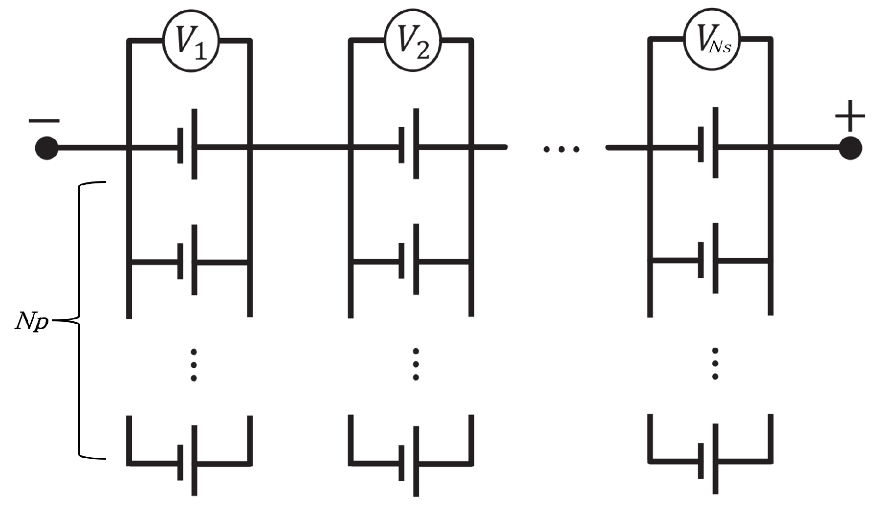
The structure of the battery energy storage system (BESS) has $N_s$ modules connected in series. Each module has $N_p$ cells connected in parallel, just like the structure shown in Figure 1. This setup is common in large battery systems. The system has two types of measurements. Voltage sensors measure electrical properties at each module. Temperature sensors monitor thermal conditions at each cell. Voltage represents overall electrical behavior, while temperature shows local thermal conditions.

Figure 1. The structure of the battery energy storage system.

2.2. Problem Formulation

Battery faults create abnormal patterns that spread through the system over time and space [26]. Heat spreads between cells [27], and electrical coupling affects multiple modules. The method collects time series data from both voltage and temperature sensors. The voltage data $\mathbf{V}\left(t\right)$ contains measurements from all modules. The temperature data $\mathbf{T}\left(t\right)$ contains readings from all cells. The goal is to find when faults occur. The method detects faults when the indicator $\mathcal{F}\left(t\right)$ exceeds a threshold ${\mathcal{F}}_{\mathrm{th}}$. After detecting a fault at time $t_f$, this research needs to find its location. This research determines which module $i_f$ and which cell $j_f$ contain the fault. This requires analyzing both voltage and temperature patterns to identify the fault coordinates.

3. Methodology

The Bayesian–Kalman fusion framework consists of four main parts, as shown in Figure 2. First, this framework uses partial least squares to extract spatiotemporal temperature patterns by calculating voltage correlation coefficients to extract voltage features. Then, Bayesian and Kalman methods are used to optimize the fusion weights. Finally, faults are accurately located through time window analysis.

Figure 2. Flowchart of the proposed method.

3.1. Partial Least Squares-Based Spatiotemporal Feature Extraction

Temperature sensors give information about thermal problems across space and time. The proposed method uses partial least squares (PLS) to analyze temperature patterns. PLS is better than traditional principal component analysis because it considers how current temperatures relate to previous temperatures [28]. This helps capture how thermal problems develop over time.

The PLS decomposition constructs latent variables that maximize covariance between input and output matrices:

$$\begin{array}{c}\hfill ({\mathbf{w}}_k,{\mathbf{q}}_k)=arg\underset{\parallel \mathbf{w}\parallel =1,\parallel \mathbf{q}\parallel =1}{max}\mathrm{Cov}(\mathbf{X}\mathbf{w},\mathbf{Y}\mathbf{q})\end{array}$$

(1)

where ${\mathbf{w}}_k\in {\mathbb{R}}^{n_x}$ is the k-th input weight vector loading weights for temperature features, ${\mathbf{q}}_k\in {\mathbb{R}}^{n_y}$ is the k-th output weight vector loading weights for lagged temperature responses, $\mathbf{X}\in {\mathbb{R}}^{n\times n_x}$ represents the centered input temperature matrix at time $t-1$ with n time samples and $n_x$ temperature sensors, $\mathbf{Y}\in {\mathbb{R}}^{n\times n_y}$ represents the centered output temperature matrix at time t with $n_y$ temperature responses, and Cov represents the covariance function between projected input and output spaces.

The NIPALS algorithm is employed for PLS decomposition due to its superior numerical stability and computational efficiency compared to eigenvalue decomposition methods, particularly when dealing with ill-conditioned or rank-deficient temperature covariance matrices that commonly arise in battery systems with redundant sensors or highly correlated thermal measurements. Unlike singular value decomposition (SVD), which requires computation of the entire covariance matrix ${\mathbf{X}}^T\mathbf{Y}$ and its eigenstructure, NIPALS performs sequential deflation where each latent variable is extracted iteratively by power iteration, making it robust to missing data and numerical singularities. The theoretical foundation lies in the alternating least squares principle: NIPALS minimizes the residual variance at each iteration by alternately solving for input weights ${\mathbf{w}}_k$ and output weights ${\mathbf{q}}_k$ that maximize the covariance $\mathrm{Cov}(\mathbf{X}\mathbf{w},\mathbf{Y}\mathbf{q})$, converging to the optimal solution through successive approximations. This iterative refinement naturally handles multicollinearity among temperature sensors without matrix inversion instability. The nonlinear iterative partial least squares (NIPALS) algorithm computes the score vectors and loading vectors:

$$\begin{array}{cc}\hfill {\mathbf{t}}_k& ={\mathbf{X}}_k{\mathbf{w}}_k,{\mathbf{p}}_k={\displaystyle \frac{{\mathbf{X}}_k^T{\mathbf{t}}_k}{{\mathbf{t}}_k^T{\mathbf{t}}_k}}\hfill \end{array}$$

(2)

where ${\mathbf{t}}_k\in {\mathbb{R}}^n$ is the k-th score vector, representing the projected temperature data onto the k-th latent variable to capture the dominant spatiotemporal patterns, ${\mathbf{X}}_k\in {\mathbb{R}}^{n\times n_x}$ is the residual temperature matrix after removing the first $k-1$ components, ${\mathbf{w}}_k\in {\mathbb{R}}^{n_x}$ is the k-th weight vector, which is the direction of maximum variance, ${\mathbf{p}}_k\in {\mathbb{R}}^{n_x}$ is the k-th loading vector, describing how each temperature sensor contributes to the k-th latent variable, ${\mathbf{X}}_k^T$ denotes the transpose of the residual matrix, and the denominator ${\mathbf{t}}_k^T{\mathbf{t}}_k$ normalizes the loading vector by the squared magnitude of the score vector.

This PLS-NIPALS approach fundamentally differs from traditional spatiotemporal feature separation methods in three aspects. First, conventional methods such as empirical orthogonal function decomposition or proper orthogonal decomposition perform spatial-only decomposition by treating time as an independent dimension, requiring explicit construction of spatial correlation matrices that ignore temporal causality. In contrast, PLS-NIPALS intrinsically captures temporal dependencies by regressing current temperature states $\mathbf{Y}\left(t\right)$ on lagged states $\mathbf{X}(t-1)$, encoding thermal propagation dynamics directly into the latent structure. Second, wavelet-based or Fourier-based spatiotemporal decomposition methods separate spatial and temporal frequencies independently, assuming linearity and stationarity that do not hold for thermal fault evolution in battery packs where nonlinear electrochemical–thermal coupling dominates. PLS-NIPALS makes no stationarity assumption and extracts latent variables that simultaneously maximize spatiotemporal covariance, capturing coupled dynamics that cannot be decomposed into separable spatial and temporal modes. Third, tensor decomposition methods such as Tucker requires multi-way data structures and face exponential computational complexity, whereas PLS-NIPALS operates on standard two-way matrices with linear complexity per iteration, making it suitable for real-time battery monitoring applications with limited computational resources.

The dual PLS statistics are computed as follows: $\xi \left(t\right)={\mathbf{t}}_t^T{\mathbf{\Lambda }}^{-1}{\mathbf{t}}_t$ (dominant statistic) and $\delta \left(t\right)=\left|\right|{\mathbf{x}}_t-\mathbf{T}{\mathbf{P}}^T{\left|\right|}^2$ (residual statistic), where ${\mathbf{t}}_t={\mathbf{x}}_t\mathbf{W}$ represents the transformed temperature features. Here, $\xi \left(t\right)$ is the dominant statistic measuring deviations in the dominant subspace, ${\mathbf{t}}_t\in {\mathbb{R}}^{n_{comp}}$ is the score vector at time t with $n_{comp}$ dominant components, $\mathbf{\Lambda }\in {\mathbb{R}}^{n_{comp}\times n_{comp}}$ is the diagonal matrix of eigenvalues $[{\lambda }_1,{\lambda }_2,...,{\lambda }_{n_{comp}}]$, representing the variance captured by each component, $\delta \left(t\right)$ is the residual statistic measuring reconstruction residuals in the orthogonal subspace, ${\mathbf{x}}_t\in {\mathbb{R}}^{n_x}$ is the centered temperature vector at time t, $\mathbf{T}\in {\mathbb{R}}^{n_{train}\times n_{comp}}$ is the score matrix from training data, $\mathbf{P}\in {\mathbb{R}}^{n_x\times n_{comp}}$ is the loading matrix, and $\mathbf{W}\in {\mathbb{R}}^{n_x\times n_{comp}}$ is the weight matrix for transforming temperature measurements to the score space.

3.2. Module Similarity Analysis for Voltage Monitoring

Battery modules normally have similar voltage patterns because they have similar chemical processes. When a fault occurs, the faulty module’s voltage drops. This creates differences with nearby modules [29]. The method use these voltage differences to detect faults quickly.

To enhance signal quality, a controlled square wave perturbation ${\tilde{V}}_i\left(t\right)=V_i\left(t\right)+A·\mathrm{square}(2\pi t/H)$ is applied to filter noise while preserving fault dynamics. And the framework calculates similarity between neighboring modules using a sliding window approach. The method is computationally efficient. It track correlations between all adjacent module pairs to form the similarity set $\mathcal{R}\left(t\right)$. The normalized deviation indicator $r_n\left(t\right)$ is derived from the two minimum correlation coefficients, where $r_n\left(t\right)<1$ indicates normal operation and $r_n\left(t\right)\ge 1$ signals fault conditions, enabling threshold-based detection.

3.3. Bayesian–Kalman Dual-Stage Weight Optimization

A critical innovation is the dual-stage optimization strategy: Bayesian optimization for global weight exploration followed by Kalman filtering for real-time adaptation. This overcomes the limitations of static weight approaches in dynamic operating conditions.

Stage 1: Bayesian Global Search—A Gaussian process models the objective function:

$$\begin{array}{c}\hfill f\left(\mathbf{w}\right)=\alpha ·\mathrm{FAR}\left(\mathbf{w}\right)+\beta ·(1-\mathrm{ADR}\left(\mathbf{w}\right))+\gamma ·{\displaystyle \frac{\mathrm{D}\left(\mathbf{w}\right)}{{\mathrm{D}}_{max}}}\end{array}$$

(3)

where $f\left(\mathbf{w}\right)$ is the multi-objective cost function to be minimized, $\mathbf{w}={[w_1,w_2,w_3]}^T\in {\mathbb{R}}^3$ represents the fusion weights for the dominant statistic, residual statistic, and correlation statistics, respectively, with constraint $w_1+w_2+w_3=1$, $\mathrm{FAR}\left(\mathbf{w}\right)$ is the false alarm rate, calculated as the percentage of normal samples incorrectly classified as faults, $\mathrm{ADR}\left(\mathbf{w}\right)$ is the anomaly detection rate, calculated as the percentage of fault samples correctly identified, $\mathrm{D}\left(\mathbf{w}\right)$ is the detection delay, measured in time steps, ${\mathrm{D}}_{max}$ is the maximum allowable detection delay for normalization, and $\alpha ,\beta ,\gamma$ are penalty coefficients balancing the three objectives.

The Expected Improvement acquisition function guides exploration:

$$\begin{array}{c}\hfill \mathrm{EI}\left(\mathbf{w}\right)=\sigma \left(\mathbf{w}\right)[Z·\mathrm{\Phi }(Z)+\varphi (Z\left)\right]\end{array}$$

(4)

where $\mathrm{EI}\left(\mathbf{w}\right)$ is the Expected Improvement value, indicating the potential benefit of evaluating weight combination $\mathbf{w}$, $\sigma \left(\mathbf{w}\right)$ is the predictive standard deviation from the Gaussian process posterior at point $\mathbf{w}$, $Z={\displaystyle \frac{f_{min}-\mu \left(\mathbf{w}\right)-\xi }{\sigma \left(\mathbf{w}\right)}}$ is the standardized improvement, with $f_{min}$ being the current best objective function value, $\mu \left(\mathbf{w}\right)$ being the predictive mean from the Gaussian process, $\xi$ being the exploration parameter controlling the exploitation–exploration trade-off, $\mathrm{\Phi }(·)$ denoting the cumulative distribution function of the standard normal distribution, and $\varphi (·)$ denoting the probability density function of the standard normal distribution.

Stage 2: Kalman Real-time Tracking—The optimal Bayesian weights initialize a Kalman filter with state transition

$$\begin{array}{c}\hfill {\mathbf{x}}_{k+1}=\mathbf{F}{\mathbf{x}}_k+{\mathbf{q}}_k,{\mathbf{z}}_k=\mathbf{H}{\mathbf{x}}_k+{\mathbf{r}}_k\end{array}$$

(5)

where ${\mathbf{x}}_k={[w_1,w_2,w_3,{\dot{w}}_1,{\dot{w}}_2,{\dot{w}}_3]}^T\in {\mathbb{R}}^6$ is the state vector, including the three fusion weights $(w_1,w_2,w_3)$ for the dominant statistic, residual statistic, and correlation statistics and their time derivatives $({\dot{w}}_1,{\dot{w}}_2,{\dot{w}}_3)$ to capture weight change dynamics, $\mathbf{F}\in {\mathbb{R}}^{6\times 6}$ is the state transition matrix, which is the identity matrix under the constant weight assumption, ${\mathbf{q}}_k\sim \mathcal{N}(\mathbf{0},\mathbf{Q})$ is the process noise vector with covariance matrix $\mathbf{Q}$, ${\mathbf{z}}_k\in {\mathbb{R}}^3$ is the observation vector, which is the noisy measurements of the weights, $\mathbf{H}\in {\mathbb{R}}^{3\times 6}$ is the observation matrix, which maps the state to observations by selecting only the weight components, and ${\mathbf{r}}_k\sim \mathcal{N}(\mathbf{0},\mathbf{R})$ is the observation noise vector with covariance matrix $\mathbf{R}$.

The core Kalman innovations are embodied in two key equations. The prediction-update cycle with performance-based feedback:

$$\begin{array}{cc}\hfill {\mathbf{P}}_{k|k-1}& =\mathbf{F}{\mathbf{P}}_{k-1}{\mathbf{F}}^T+\mathbf{Q}\hfill \end{array}$$

(6)

$$\begin{array}{cc}\hfill {\mathbf{K}}_k& ={\mathbf{P}}_{k|k-1}{\mathbf{H}}^T{(\mathbf{H}{\mathbf{P}}_{k|k-1}{\mathbf{H}}^T+\mathbf{R})}^{-1}\hfill \end{array}$$

(7)

where ${\mathbf{P}}_{k|k-1}\in {\mathbb{R}}^{6\times 6}$ is the predicted error covariance matrix, representing the uncertainty in weight estimates before incorporating new observations, ${\mathbf{P}}_{k-1}\in {\mathbb{R}}^{6\times 6}$ is the previous posterior error covariance matrix, ${\mathbf{F}}^T$ is the transpose of the state transition matrix, $\mathbf{Q}$ is the process noise covariance matrix, accounting for weight variation, ${\mathbf{K}}_k\in {\mathbb{R}}^{6\times 3}$ is the Kalman gain matrix, determining the optimal balance between prediction and observation, ${\mathbf{H}}^T$ is the transpose of the observation matrix, $\mathbf{R}$ is the observation noise covariance matrix, reflecting measurement uncertainty, and the inverse term ${(\mathbf{H}{\mathbf{P}}_{k|k-1}{\mathbf{H}}^T+\mathbf{R})}^{-1}$ represents the innovation covariance used for gain normalization.

The adaptive weight evolution with multi-objective performance feedback:

$$\begin{array}{c}\hfill {\mathbf{z}}_k=\left\{\begin{array}{cc}{\kappa }_1{\mathbf{x}}_{k|k-1}+{\kappa }_2{\mathbf{w}}_{Bayes}\hfill & \mathrm{if}{\mathcal{J}}_k>{\mathcal{J}}_{k-1}\hfill \\ {\mathbf{x}}_{k|k-1}+ϵ{\mathit{\eta }}_k\hfill & \mathrm{if}{\mathcal{J}}_k\le {\mathcal{J}}_{k-1}\hfill \end{array}\right.\end{array}$$

(8)

where ${\mathbf{z}}_k\in {\mathbb{R}}^3$ is the adaptive observation vector containing the weight measurements at time k, ${\mathbf{x}}_{k|k-1}\in {\mathbb{R}}^6$ is the predicted state vector, with the first 3 components extracted for observation, ${\mathbf{w}}_{Bayes}\in {\mathbb{R}}^3$ represents the optimal Bayesian weights, serving as a reference anchor when performance degrades, ${\mathcal{J}}_k$ is the current multi-objective performance cost function value incorporating ADR, FAR, and detection delay metrics, ${\mathcal{J}}_{k-1}$ is the previous performance cost for comparison, the coefficients ${\kappa }_1$ and ${\kappa }_2$ control the balance between predicted state and Bayesian reference when performance degrades, ${\mathit{\eta }}_k\sim \mathcal{N}(\mathbf{0},{\mathbf{I}}_3)$ is a zero-mean Gaussian noise vector for controlled exploration, and the small coefficient $ϵ$ ensures minimal exploration when performance is improving.

The final multiscale indicator is $\mathcal{F}\left(t\right)=w_1^{*}\xi \left(t\right)/{\xi }_{UCL}+w_2^{*}\delta \left(t\right)/{\delta }_{UCL}+w_3^{*}{r}_n\left(t\right)$, where $\mathcal{F}\left(t\right)$ is the normalized fusion metric for fault detection, with $\mathcal{F}\left(t\right)>1$ indicating fault conditions, $w_1^{*}\in [0,1]$ is the Kalman-optimized weight for the PLS dominant statistic $\xi \left(t\right)$, $w_2^{*}\in [0,1]$ is the Kalman-optimized weight for the PLS residual statistic $\delta \left(t\right)$, $w_3^{*}\in [0,1]$ is the Kalman-optimized weight for the voltage correlation deviation $d_n\left(t\right)$, ${\xi }_{UCL}$ is the upper control limit for the dominant statistic, calculated from training data, ${\delta }_{UCL}$ is the upper control limit for the residual statistic, $r_n\left(t\right)\le 1$ represents the normalized voltage correlation deviation, and ${\mathbf{w}}^{*}=[w_1^{*},w_2^{*},w_3^{*}]$ satisfies the constraint $w_1^{*}+w_2^{*}+w_3^{*}=1$, with weights dynamically adapted by the Kalman filter.

3.4. Time Window-Based Fault Localization

The proposed fault localization strategy operates in two stages: module-level module identification and cell-level cell localization using time window analysis.

3.4.1. Module Identification via Correlation Analysis

The module-level localization analyzes module voltage correlation degradation. When internal short-circuit faults occur, the affected module experiences correlation drops with adjacent modules. The algorithm identifies fault modules by monitoring voltage correlation patterns in a time window and detecting simultaneous correlation degradation between the fault module and its adjacent modules.

The voltage contribution for each module is quantified by counting low correlation occurrences within a time window following fault detection. For module i, the raw voltage contribution is computed as follows:

$$\begin{array}{c}\hfill C_i^r=\sum _{t=t_f}^{t_f+W}\mathbb{I}(r_i\left(t\right)<r_{th})\end{array}$$

(9)

where $C_i^r$ is the raw voltage contribution, counting correlation degradation events, $t_f$ is the fault detection time, W is the analysis window length, $r_i\left(t\right)$ is the correlation coefficient between module i and its adjacent module at time t, $r_{th}$ is the low correlation threshold, and $\mathbb{I}(·)$ is the indicator function, returning 1 when the condition is true and 0 otherwise. The final module contribution considers spatial adjacency effects:

$$\begin{array}{c}\hfill C_i^{module}={\displaystyle \frac{C_i^r+C_{i+1}^r}{2}}\end{array}$$

(10)

where $C_i^{module}$ is the smoothed voltage contribution for module i, accounting for fault propagation to neighboring modules, and $i+1$ denotes the next module in the series connection with cyclic indexing. The faulty module is identified as $i_f=arg{max}_i{C}_i^{module}$, where the module with the maximum voltage contribution indicates the fault location. This averaging operation enhances localization robustness by accounting for the fact that a fault in module i causes correlation degradation in both $(i-1,i)$ and $(i,i+1)$ pairs, creating overlapping signatures that pinpoint the common faulty module.

3.4.2. Time Window-Based Cumulative Contribution Analysis

The cell-level localization introduces time window cumulative contribution analysis, a key innovation addressing noise-sensitive instantaneous detection. After fault detection, the method analyzes temperature patterns within a time window to calculate cumulative anomaly contributions for each sensor. The multi-dimensional contribution combines normalized temperature deviations, absolute temperature changes, and temperature rise indicators to identify the fault cell location robustly.

The comprehensive contribution integrates PLS-based dominant and residual contributions:

$$\begin{array}{c}\hfill C_{\xi }\left(j\right)=\sum _{k=1}^{n_{comp}}{\displaystyle \frac{|s_k{p}_{kj}{x}_j|}{{\lambda }_k}},C_{\delta }\left(j\right)=e_j^2\end{array}$$

(11)

where $C_{\xi }\left(j\right)$ is the contribution of the j-th sensor to the PLS dominant statistic, measuring how much the sensor deviates in the dominant subspace, $n_{comp}$ is the number of dominant components retained in the PLS model, $s_k$ is the k-th score value from the score vector ${\mathbf{t}}_t$, $p_{kj}$ is the loading coefficient connecting the k-th dominant component to the j-th sensor (element of loading matrix $\mathbf{P}$), $x_j$ is the centered temperature measurement from the j-th sensor, ${\lambda }_k$ is the k-th eigenvalue, representing the variance captured by the k-th component, $C_{\delta }\left(j\right)=e_j^2$ is the contribution of the j-th sensor to the PLS residual statistic, and $e_j$ is the reconstruction residual for the j-th sensor, calculated as $e_j=x_j-{\sum }_{k=1}^{n_{comp}}{s}_k{p}_{kj}$, representing the part of temperature variation not captured by the PLS model.

The fault cell identification uses the maximum cumulative contribution:

$$\begin{array}{c}\hfill c_f=arg\underset{j}{max}\left[{\displaystyle \frac{w_1{C}_{\xi }\left(j\right)+w_2{C}_{\delta }\left(j\right)}{w_1+w_2}}+C_j^{cum}\right]\end{array}$$

(12)

where $c_f$ is the identified fault cell index within the faulty module, $arg{max}_j$ finds the sensor index j that maximizes the combined contribution score, $w_1$ and $w_2$ are the Kalman-optimized weights for the PLS dominant and residual statistics, respectively, ${\displaystyle \frac{w_1{C}_{\xi }\left(j\right)+w_2{C}_{\delta }\left(j\right)}{w_1+w_2}}$ represents the weighted average of PLS-based contributions normalized by the sum of PLS weights, and the addition of $C_j^{cum}$ incorporates the time window cumulative temperature anomaly analysis to enhance localization robustness by reducing sensitivity to instantaneous measurement noise. The hierarchical approach reduces computational complexity by first narrowing to the faulty module (from $N_s$ candidates) and then precisely localizing the specific cell within that module (from $N_p$ candidates), achieving both efficiency and accuracy.

4. Experimental Verification

4.1. Experimental Dataset and Setup

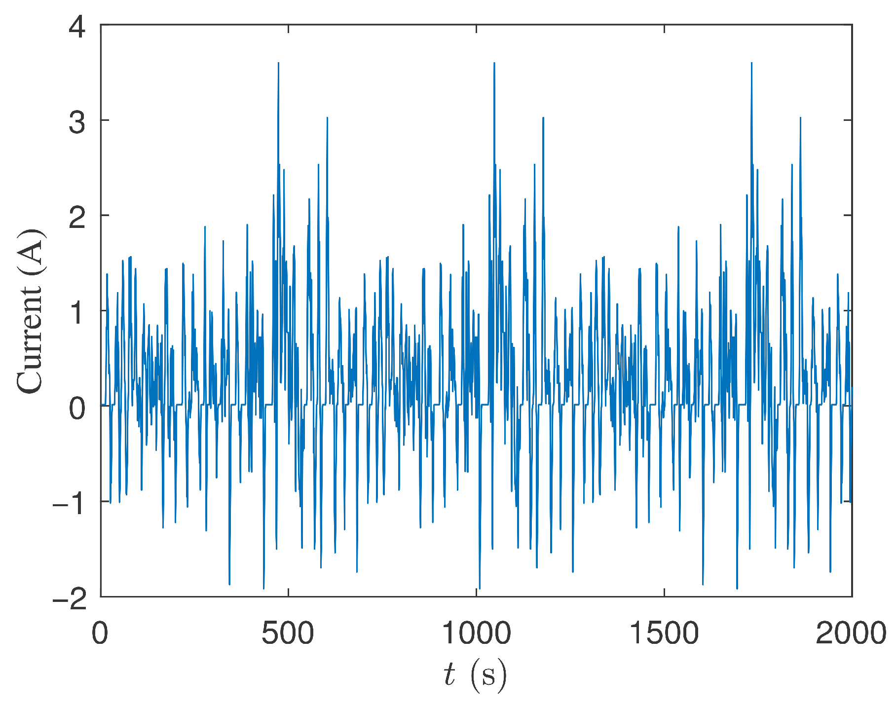
The experimental verification adopted a 6S4P Li-ion battery configuration and simulated six fault scenarios under various conditions, including the UDDS dynamic curve, as shown in Table 1. The current variation of UDDS is depicted in Figure 3. Due to the high cost, danger, and poor repeatability of internal short-circuit thermal failure experiments, a simulation equivalent method as outlined in [30] is used to simulate the failure scenarios occurring in the battery pack. The proposed method connects resistors in parallel at both ends of the battery to simulate internal short circuit. The data was collected at a frequency of one time per second, with a total of 2000 data points collected. Gaussian white noise was also added to simulate the real measurement conditions. In the weight optimization phase, 60% of the time points are randomly selected as the test set data. The equipment used in the experiment is shown in Figure 4, including a Li-ion battery system that contains sensors capable of measuring voltage and temperature data, a charging and discharging device that simulates the current variation, and a constant temperature box that simulates the temperature environment.

Table 1. Fault condition settings.

Fault No.	Current	${\mathit{R}}_{\mathit{short}}$	Time of Fault Occurrence	Fault Position ${\mathit{z}}_{\mathit{f}}$
#1	2C	10 $\mathrm{\Omega }$	1000	[1,4]
#2	2C	10 $\mathrm{\Omega }$	1000	[2,1]
#3	2C	5 $\mathrm{\Omega }$	1000	[6, 3]
#4	1C	10 $\mathrm{\Omega }$	1000	[6,3]
#5	UDDS	10 $\mathrm{\Omega }$	1000	[6,3]
#6	2C	20 $\mathrm{\Omega }$	1000	[6,3]

Figure 3. Current variation under UDDS.

Figure 4. Experimental equipment diagram.

The six fault scenarios comprehensively evaluate the framework’s performance across different operating conditions, fault severities, and spatial locations, systematically spanning the fault evolution spectrum from early-stage weak faults to critical strong faults. Fault #1 occurs at module 1, cell 4 with medium short-circuit resistance 10 $\mathrm{\Omega }$ under 2C constant current discharge, representing a typical moderate-severity fault at the first module position. Fault #2 is located at module 2, cell 1 with the same 10 $\mathrm{\Omega }$ medium resistance and 2C current, examining detection performance at a different spatial location with moderate thermal stress. Fault #3 tests the framework’s capability to detect strong faults by employing a low short-circuit resistance of 5 $\mathrm{\Omega }$ at module 6, cell 3 under 2C discharge, representing a severe thermal fault condition with rapid temperature escalation approaching critical failure thresholds. Fault #4 evaluates performance under reduced current conditions of 1C with 10 $\mathrm{\Omega }$ medium resistance at module 6, cell 3, examining the impact of lower discharge rates on fault detection with moderate severity. Fault #5 represents the most challenging scenario by introducing internal short circuit with 10 $\mathrm{\Omega }$ medium resistance under dynamic UDDS driving cycle conditions, testing the framework’s robustness against time-varying currents and complex operating patterns with moderate thermal risk. Fault #6 tests the framework’s sensitivity to weak faults by employing a high short-circuit resistance of 20 $\mathrm{\Omega }$ at module 6, cell 3 under 2C discharge, simulating early-stage thermal degradation where there is still a considerable amount of time before thermal runaway occurs, representing the most benign fault condition requiring early warning capabilities.

Algorithm Parameter Configuration

The proposed framework involves multiple algorithmic components requiring careful parameter tuning. Table 2 summarizes the key parameters and their values used in the experimental validation. To simulate realistic measurement conditions, Gaussian white noise is added to both voltage and temperature data with signal-to-noise ratios (SNRs) of 90 dB for voltage and 50 dB for temperature measurements. The voltage SNR of 90 dB corresponds to a noise standard deviation of approximately 0.01% of the signal amplitude, reflecting high-precision voltage sensors typically used in battery management systems. The lower temperature SNR of 50 dB, noise standard deviation approximately 0.3% of the signal amplitude, accounts for the inherently higher measurement uncertainty in thermal sensors due to thermal contact resistance, ambient temperature fluctuations, and sensor response time. These noise levels are representative of practical battery monitoring systems and enable robust evaluation of the framework’s noise immunity.

Table 2. Algorithm parameter settings.

Component	Parameter	Symbol	Value
Measurement Noise	Voltage SNR	SNRV	90 dB
	Temperature SNR	SNRT	50 dB
PLS Analysis	Number of sensors	$n_x$	24
	Principal components	$n_{comp}$	6
	Training samples	$n_{train}$	800
	Test samples	$n_{test}$	1200
Bayesian Optimization	FAR penalty	$\alpha$	80
	ADR penalty	$\beta$	60
	Delay penalty	$\gamma$	0.05
Kalman Filtering	Process noise	$\mathbf{Q}$	$2\times {10}^{-4}{\mathbf{I}}_6$
	Observation noise	$\mathbf{R}$	$5\times {10}^{-3}{\mathbf{I}}_3$
	Degradation coefficient	${\kappa }_1$	0.8
	Reference coefficient	${\kappa }_2$	0.2
	Exploration coefficient	$ϵ$	0.005
Time Window Localization	Analysis window	W	50
	Z-score weight	$\alpha$	0.3
	Deviation weight	$\beta$	0.3
	Rise indicator weight	$\gamma$	0.2

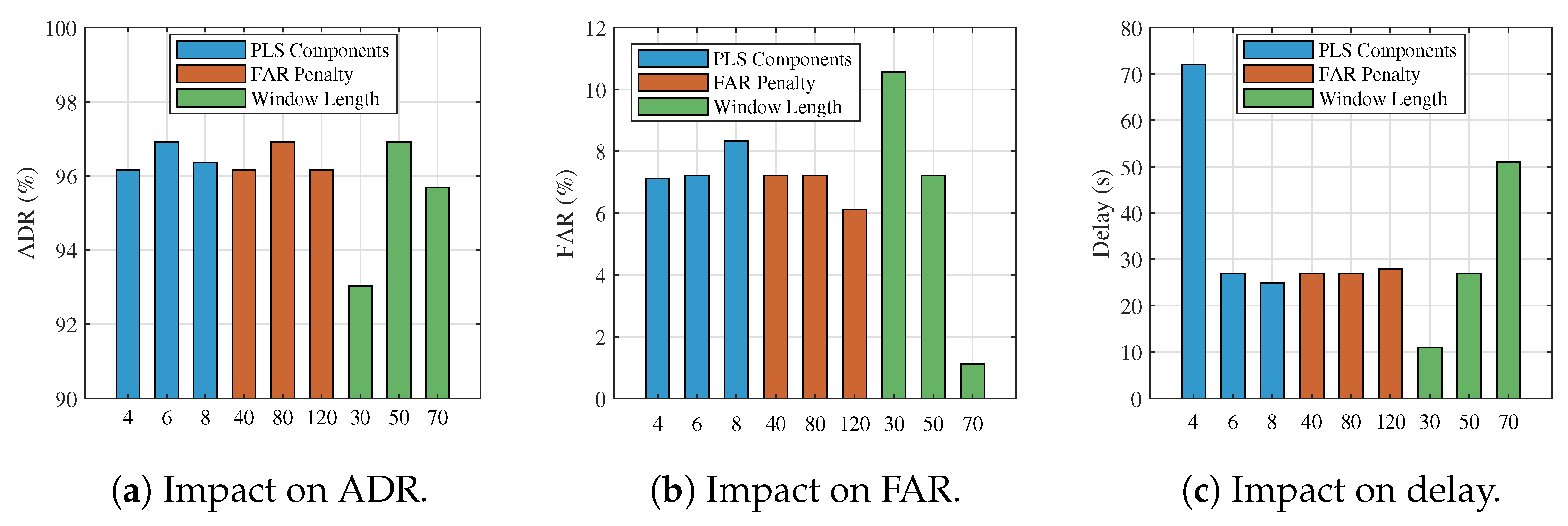
The parameter selection is based on the following considerations: PLS components: Six components are retained to capture 95% of temperature variance while avoiding overfitting, determined through cross-validation analysis. Bayesian penalty coefficients: The weights $\alpha =80,\beta =60,\gamma =0.05$ prioritize false alarm reduction over detection delay, suitable for safety-critical battery applications where false alarms cause unnecessary shutdowns. Kalman noise parameters: Process noise $\mathbf{Q}=2\times {10}^{-4}\mathbf{I}$ allows moderate weight variation to adapt to changing conditions, while observation noise $\mathbf{R}=5\times {10}^{-3}\mathbf{I}$ reflects realistic measurement uncertainty. The degradation coefficients ${\kappa }_1=0.8,{\kappa }_2=0.2$ provide strong stabilization toward predicted weights with moderate Bayesian reference influence. Localization parameters: Window length $W=50$ balances noise reduction with temporal resolution, while the contribution weights $\alpha =0.3,\beta =0.3,\gamma =0.2$ emphasize statistical deviations over temperature rise patterns for robust localization.

To validate the robustness and optimality of the selected parameters, a comprehensive cross-validation analysis was conducted on Fault #5 under UDDS dynamic conditions, which represents the most challenging scenario with time-varying current profiles. Figure 5 presents the performance sensitivity across three critical parameter groups: PLS principal components, FAR penalty coefficients in Bayesian optimization, and time window analysis length. The results demonstrate that the framework exhibits stable performance across a wide parameter range, with the selected values achieving an optimal balance across all three performance metrics. Specifically, six PLS components capture 95% of temperature variance while maintaining ADR above 96% and FAR below 8%, avoiding both underfitting from insufficient components and overfitting from excessive components. The FAR penalty coefficient of 80 provides the lowest false alarm rate of 7.22% while preserving high detection capability, validating the framework’s emphasis on false alarm reduction for safety-critical applications. The 50-sample time window achieves a superior ADR-FAR trade-off with minimal detection delay, effectively filtering transient noise-induced fluctuations while maintaining temporal resolution for rapid fault response. This cross-validation analysis confirms the parameter selection methodology based on multi-objective optimization principles and establishes confidence intervals for deployment across diverse battery systems and operating conditions.

Figure 5. Cross-validation analysis of algorithm parameter sensitivity under Fault #5.

4.2. Fault Detection Results

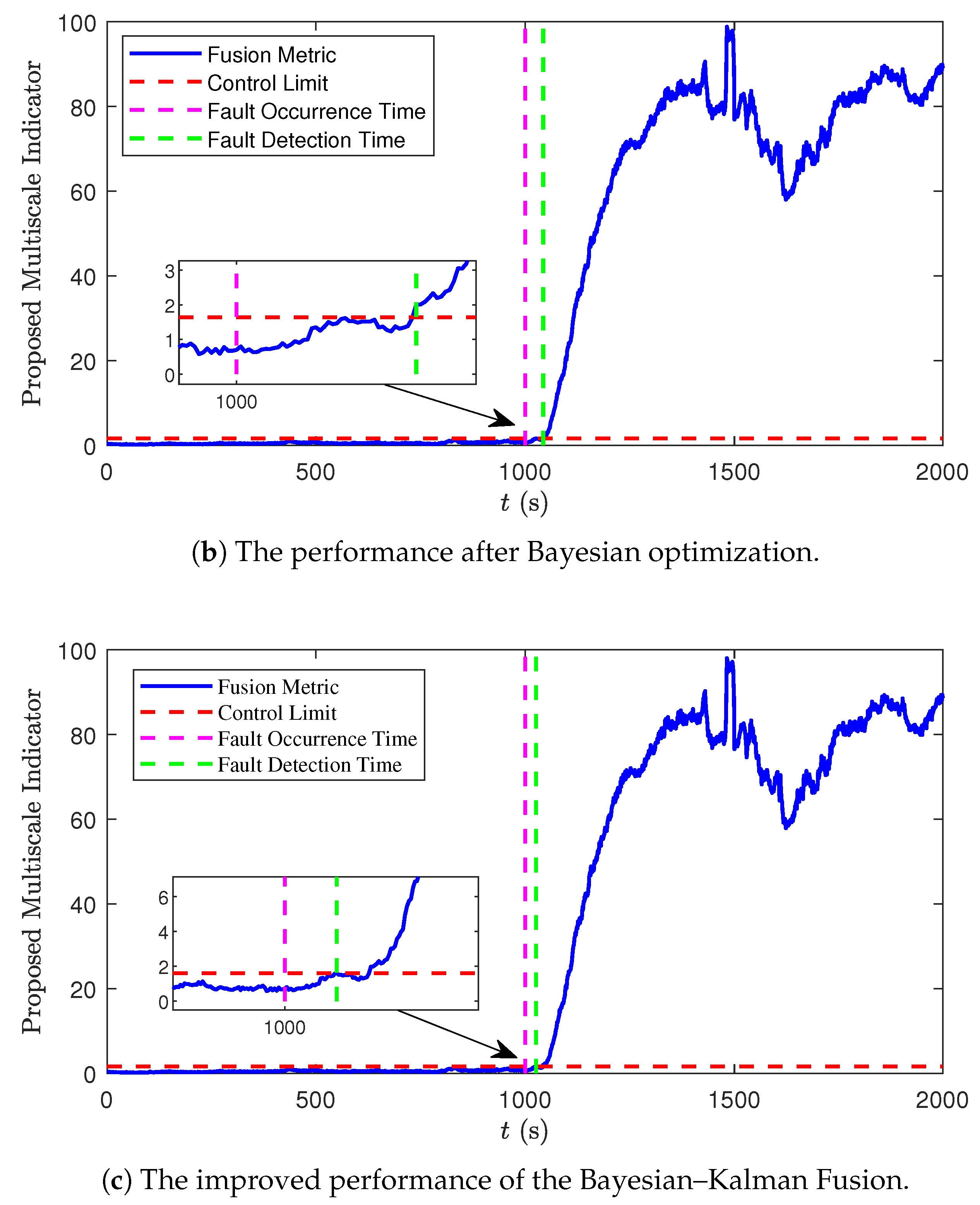
Figure 6 illustrates the Bayesian optimization convergence process for Faults #4 and #5. Fault #4 converges rapidly to a stable state below 3 after 50 iterations, and Fault #5 also converges quickly and reaches a stable state after 50 iterations. Figure 7 demonstrates the progressive performance improvement from initial weights through Bayesian optimization to the final Bayesian–Kalman fusion. The result indicates that its stability has been enhanced, the fault detection capability has become clearer, and the fluctuations caused by noise have been reduced. The weights before Bayesian optimization would lead to premature detection of faults being wrongly identified. After fine-tuning with Kalman filtering, the detection delay was significantly reduced.

Figure 6. Bayesian optimization process.

Figure 7. Performance comparison of different weight optimizations under the UDDS scenario.

The computational efficiency of the proposed framework was evaluated on a workstation equipped with Intel Core i9-13900HX CPU and 16GB RAM. For the complete dataset containing 2000 time points, the average execution time for the fault detection algorithm was 3.46 s, corresponding to approximately 1.73 ms per time point. This computational efficiency demonstrates the framework’s suitability for real-time battery monitoring applications, where the processing speed significantly exceeds the typical data acquisition rate of 1 Hz used in battery management systems. The low computational overhead enables deployment on embedded platforms with moderate processing capabilities while maintaining a sufficient margin for concurrent execution of other battery management functions such as state estimation and thermal control.

Table 3 demonstrates the superior performance of the Bayesian–Kalman fusion framework across all fault scenarios spanning different severity levels. This framework achieves ADR from 96.92% to 99.90%, with FAR ranging from 0.10% to 7.22% and reduced detection latency to 1–27 s. The optimal weight combinations vary significantly across fault severities and types, revealing intelligent adaptation to fault characteristics. For strong faults, Fault #3, the framework emphasizes temperature-based dominant statistics with $w_1=0.747$, effectively capturing rapid thermal escalation patterns approaching thermal runaway. For medium faults, weight distributions adapt to specific operating conditions. Most notably, for weak faults, Fault #6, representing early-stage degradation with extended time before thermal runaway, the framework maintains high detection performance despite minimal thermal signatures, demonstrating exceptional sensitivity for early warning. In the UDDS dynamic environment, unoptimized initial weights can lead to premature false alarms in fault detection, and the fusion indicators may lose their anti-interference ability, resulting in the failure of fault detection, as indicated by ‘N/A’ in the table.

Table 3. Comprehensive performance comparison of detection methods.

Fault No.	Optimization	${\mathit{w}}_1$	${\mathit{w}}_2$	${\mathit{w}}_3$	ADR (%)	FAR (%)	Delay (s)
#1	Original weight	0.400	0.400	0.200	99.50	2.00	2
	Bayesian optimization	0.516	0.223	0.261	99.80	1.80	2
	Bayesian–Kalman Fusion	0.492	0.235	0.273	99.90	1.80	1
#2	Original weight	0.400	0.400	0.200	95.14	0.40	2
	Bayesian optimization	0.053	0.396	0.551	99.70	0.10	2
	Bayesian–Kalman Fusion	0.032	0.398	0.570	99.70	0.10	2
#3	Original weight	0.400	0.400	0.200	99.80	1.80	2
	Bayesian optimization	0.762	0.188	0.050	99.80	1.70	2
	Bayesian–Kalman Fusion	0.747	0.189	0.065	99.90	1.70	2
#4	Original weight	0.400	0.400	0.200	99.90	2.10	2
	Bayesian optimization	0.705	0.233	0.062	99.90	0.50	1
	Bayesian–Kalman Fusion	0.695	0.231	0.074	99.90	0.30	1
#5	Original weight	0.400	0.400	0.200	97.45	32.33	N/A
	Bayesian optimization	0.113	0.118	0.787	96.86	11.67	44
	Bayesian–Kalman Fusion	0.125	0.114	0.759	96.92	7.22	27
#6	Original weight	0.400	0.400	0.200	99.60	1.80	4
	Bayesian optimization	0.253	0.318	0.429	99.50	0.60	5
	Bayesian–Kalman Fusion	0.247	0.315	0.438	99.50	0.60	5

4.3. Fault Localization Results

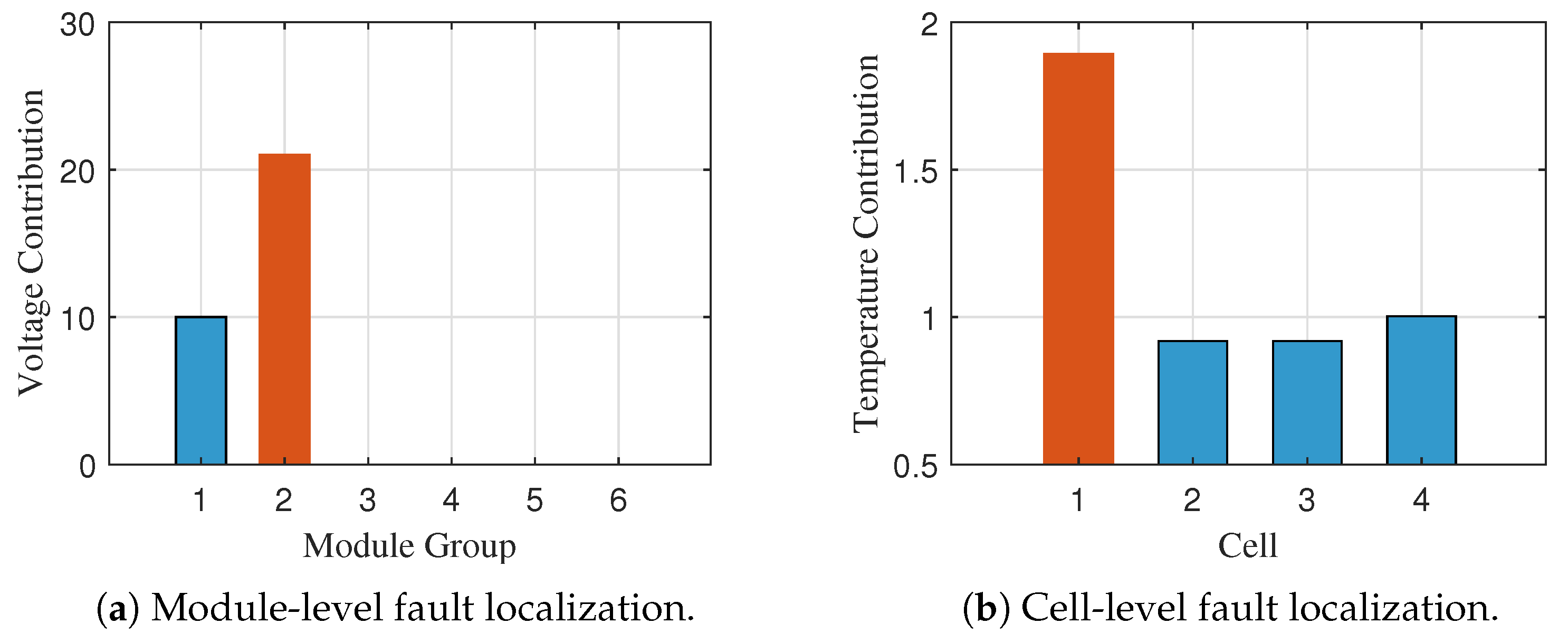
The hierarchical fault localization approach achieves exceptional accuracy through two-stage analysis combining voltage correlation for module identification and time window cumulative contribution for cell localization. Figure 8a,b show successful identification of Fault #2 at module 2, cell 1, with a clear distinction between faulty and healthy components. Figure 9 demonstrates consistent localization performance for Fault #5 at module 6, cell 3, with clear identification through correlation degradation and cumulative contribution analysis. The 50 s time window approach provides robust noise immunity while maintaining accurate spatial resolution.

Figure 8. Fault localization results under Fault #2. (The orange bar denotes the maximum value corresponding to the identified faulty battery module in Figure 8a and the identified faulty battery cell in Figure 8b).

Figure 9. Fault localization results under Fault #4. (The orange bar denotes the maximum value corresponding to the identified faulty battery module in Figure 9a and the identified faulty battery cell in Figure 9b).

Table 4 demonstrates 100% localization accuracy across all five fault scenarios, spanning diverse spatial positions and operating conditions, including challenging UDDS dynamic profiles. The consistent performance across different fault severities and locations validates the robustness of the hierarchical localization approach.

Table 4. Fault localization results.

Fault No.	Module Position ${\mathit{i}}_{\mathit{f}}$	Cell Position ${\mathit{j}}_{\mathit{f}}$	Result
#1	1	4	Correct
#2	2	1	Correct
#3	6	3	Correct
#4	6	3	Correct
#5	6	3	Correct

5. Results Analysis and Discussion

The experimental results demonstrate significant performance improvements through the proposed Bayesian–Kalman fusion approach, achieving ADR values of 96.92–99.90% with FAR ranging from 0.10% to 7.22% across all fault scenarios spanning three distinct severity levels. The adaptive weight optimization reveals distinct fault severity signatures, validating the importance of intelligent sensor fusion strategies. Most significantly, for weak faults with 20 $\mathrm{\Omega }$ resistance, Fault #6, representing early-stage degradation with extended time before thermal runaway, the framework demonstrates exceptional early warning capability with 99.50% ADR and 0.60% FAR despite minimal thermal signatures, enabling proactive intervention long before critical failure thresholds. The hierarchical localization approach achieves perfect 100% accuracy across all severity levels, with detection delays of 1–27 s demonstrating real-time implementation capability. The framework shows particular effectiveness under challenging UDDS dynamic conditions, where false alarm rates drop from 32.33% to 7.22% and detection delays improve from unstable values to 27 s, highlighting the robustness of the time window cumulative analysis and adaptive optimization mechanisms.

To comprehensively evaluate the framework’s robustness under varying measurement noise conditions, a systematic noise sensitivity analysis was conducted across different signal-to-noise ratio levels. Figure 10 presents the performance variation using violin plots that visualize the probability density distribution of ADR, FAR, and detection delay under three noise scenarios with a voltage SNR of 70 dB, 75 dB, and 80 dB combined with a temperature SNR of 40 dB, 45 dB, and 50 dB, respectively. The ADR remains consistently high above 96% across all noise levels with narrow distribution width, demonstrating robust fault detection capability even under severe measurement noise. The FAR shows an expected increase with higher noise levels but remains below 8% even under the most challenging conditions, while median values stay below 2% for moderate- and low-noise scenarios. The detection delay exhibits a slight increase from 1–3 s under low noise to 5–10 s under high-noise conditions. These results confirm the framework’s ability to maintain stable performance through the Bayesian–Kalman fusion mechanism and time window cumulative analysis that effectively filters transient noise-induced fluctuations while preserving genuine fault sensitivity.

Figure 10. Noise robustness analysis.

The remarkable performance improvement under UDDS dynamic conditions can be attributed to the synergistic interaction between Bayesian global exploration and Kalman real-time adaptation. The Bayesian optimization stage identifies the optimal weight balance, assigning dominant weight-to-voltage correlation statistics $w_3=0.759$, which exhibit stronger discriminative power under rapidly varying current profiles where thermal dynamics lag behind electrical responses. This global exploration prevents suboptimal local minima that plague traditional fixed-weight approaches. Subsequently, the Kalman filtering stage provides continuous adaptation to time-varying fault characteristics through the adaptive observation mechanism, which monitors multi-objective performance metrics and adjusts weights when degradation occurs. This feedback-driven adaptation is crucial in UDDS scenarios where current fluctuations induce complex spatiotemporal thermal patterns. The integration of time window cumulative contribution analysis further mitigates transient current-induced temperature oscillations by accumulating anomaly evidence over sliding windows, effectively filtering false positives caused by legitimate thermal responses while preserving genuine fault sensitivity. This synergy achieves a 77.7% reduction in false alarm rate and establishes stable detection delays where initial weights failed completely.

The demonstrated performance of the proposed framework offers significant pathways for advancing energy sustainability through enhanced BESS safety and reliability. Integration into utility-scale renewable energy storage installations can prevent catastrophic thermal failures that undermine public confidence in clean energy infrastructure, while the 100% fault localization accuracy enables predictive maintenance strategies that extend battery lifespan, reducing the environmental footprint from premature replacement. In electric vehicle applications, the low false alarm rates of 0.10–7.22% minimize unnecessary downtime and range anxiety, directly improving EV adoption rates critical for transportation decarbonization. The framework’s real-time capability also enables dynamic thermal management optimization, potentially reducing cooling energy consumption by 20–30% through precise fault localization that eliminates wasteful system-wide responses. Furthermore, the robustness under UDDS dynamic conditions makes this approach particularly suitable for vehicle-to-grid applications, where reliable fault detection enables widespread deployment of distributed energy storage networks that stabilize renewable-dominated grids. The transfer learning potential of the Bayesian–Kalman framework allows rapid adaptation to emerging battery chemistries and configurations, accelerating validation of next-generation energy storage technologies essential for sustainable energy transitions.

6. Conclusions

This research presents a comprehensive Bayesian–Kalman fusion framework for fault detection and localization of BESSs. The proposed approach achieves exceptional performance, with 96.92–99.90% anomaly detection rates, false alarm rates of 0.10–7.22%, and 100% fault localization accuracy across diverse operating conditions. The key innovations include dual-stage optimization combining Bayesian global exploration with Kalman real-time adaptation, PLS-based spatiotemporal feature extraction, and hierarchical fault localization using time window cumulative contribution analysis. The framework demonstrates practical advantages through real-time capability with detection delays of 1–27 s. The experimental validation across six fault scenarios spanning different spatial positions, severities, and operating conditions including challenging UDDS profiles establishes the framework’s robustness and suitability for next-generation battery safety management systems in electric vehicles and utility-scale energy storage applications.

Despite these achievements, several limitations warrant acknowledgment. The current validation employs a 6S4P battery configuration with controlled internal short-circuit faults; larger-scale systems with more complex topologies and diverse fault types require further investigation. The Bayesian optimization stage involves computational overhead that may constrain real-time deployment in resource-limited embedded systems, though offline pre-optimization partially mitigates this concern. Additionally, the framework assumes availability of both voltage and temperature measurements; practical scenarios with sensor failures or missing data require robust sensor-fault-tolerant extensions. Future research directions include extending the framework to accommodate battery aging effects through adaptive threshold adjustment mechanisms that account for capacity fade and impedance growth over cycling. Investigation of transfer learning approaches could enable efficient adaptation across different battery chemistries and pack configurations without extensive retraining. Integration of physics-informed constraints into the Bayesian optimization process may enhance convergence speed and solution interpretability. Furthermore, validation on diverse fault types beyond internal short circuits, including external short circuits, overcharge conditions, and mechanical abuse scenarios, would strengthen practical applicability.

References

1. Cao, K.L.A.; Ogi, T. Advanced carbon sphere-based hybrid materials produced by innovative aerosol process for high-efficiency rechargeable batteries. Energy Storage Mater. 2025, 74, 103901. [Google Scholar] [CrossRef]
2. Nyamathulla, S.; Dhanamjayulu, C. A review of battery energy storage systems and advanced battery management system for different applications: Challenges and recommendations. J. Energy Storage 2024, 86, 111179. [Google Scholar] [CrossRef]
3. Lawder, M.T.; Suthar, B.; Northrop, P.W.C.; De, S.; Hoff, C.M.; Leitermann, O.; Crow, M.L.; Santhanagopalan, S.; Subramanian, V.R. Battery Energy Storage System (BESS) and Battery Management System (BMS) for Grid-Scale Applications. Proc. IEEE 2014, 102, 1014–1030. [Google Scholar] [CrossRef]
4. Eskandari, M.; Rajabi, A.; Savkin, A.V.; Moradi, M.H.; Dong, Z.Y. Battery energy storage systems (BESSs) and the economy-dynamics of microgrids: Review, analysis, and classification for standardization of BESSs applications. J. Energy Storage 2022, 55, 105627. [Google Scholar] [CrossRef]
5. Wang, L.; Bu, Y.; Wu, Y. Multi-Scale Risk-Informed Comprehensive Assessment Methodology for Lithium-Ion Battery Energy Storage System. Sustainability 2024, 16, 9046. [Google Scholar] [CrossRef]
6. Feng, Y.; Li, H.X. Detection and Spatial Identification of Fault for Parabolic Distributed Parameter Systems. IEEE Trans. Ind. Electron. 2019, 66, 7300–7309. [Google Scholar] [CrossRef]
7. Feng, Y.; Wang, Y.; Wan, Q.; Zhang, X.; Wang, B.C.; Li, H.X. From Online Systems Modeling to Fault Detection for a Class of Unknown High-Dimensional Distributed Parameter Systems. IEEE Trans. Ind. Electron. 2023, 70, 5317–5325. [Google Scholar] [CrossRef]
8. Qi, C.; Li, H.X.; Zhang, X.; Zhao, X.; Li, S.; Gao, F. Time/space-separation-based SVM modeling for nonlinear distributed parameter processes. Ind. Eng. Chem. Res. 2011, 50, 332–341. [Google Scholar] [CrossRef]
9. Zhou, J.; Chen, L.; Zhang, S.; Zhou, Y.; Wang, S.; Shen, W. Distributed Thermal Monitoring for Large-Format Li-Ion Battery Under Limited Sensing. IEEE Trans. Transp. Electrif. 2024, 10, 3206–3217. [Google Scholar] [CrossRef]
10. Wang, Z.; Li, H.X. Incremental spatiotemporal learning for online modeling of distributed parameter systems. IEEE Trans. Syst. Man. Cybern. Syst. 2018, 49, 2612–2622. [Google Scholar] [CrossRef]
11. Yu, Z.; Tian, Y.; Li, B. A simulation study of Li-ion batteries based on a modified P2D model. J. Power Sources 2024, 618, 234376. [Google Scholar] [CrossRef]
12. Chen, L.; Li, H.X.; Xie, S. Modified High-Order SVD for Spatiotemporal Modeling of Distributed Parameter Systems. IEEE Trans. Ind. Electron. 2022, 69, 4296–4304. [Google Scholar] [CrossRef]
13. Wei, P.; Li, H.X. Two-Dimensional Spatial Construction for Online Modeling of Distributed Parameter Systems. IEEE Trans. Ind. Electron. 2022, 69, 10227–10235. [Google Scholar] [CrossRef]
14. Stocker, R.; Mumtaz, A.; Paramjeet; Braglia, M.; Lophitis, N. Universal Li-Ion Cell Electrothermal Model. IEEE Trans. Transp. Electrif. 2021, 7, 6–15. [Google Scholar] [CrossRef]
15. Li, S.; Zhang, C.; Du, J.; Cong, X.; Zhang, L.; Jiang, Y.; Wang, L. Fault diagnosis for lithium-ion batteries in electric vehicles based on signal decomposition and two-dimensional feature clustering. Green Energy Intell. Transp. 2022, 1, 100009. [Google Scholar] [CrossRef]
16. Gupta, S.; Sahoo, A.K.; Sahoo, U.K. Wireless Sensor Network-Based Distributed Approach to Identify Spatio-Temporal Volterra Model for Industrial Distributed Parameter Systems. IEEE Trans. Ind. Inform. 2020, 16, 7671–7681. [Google Scholar] [CrossRef]
17. Wei, P.; Li, H.X. A Spatio-Temporal Inference System for Abnormality Detection and Localization of Battery Systems. IEEE Trans. Ind. Inform. 2023, 19, 6275–6283. [Google Scholar] [CrossRef]
18. Salehimehr, S.; Miraftabzadeh, S.M.; Brenna, M. A Novel Machine Learning-Based Approach for Fault Detection and Location in Low-Voltage DC Microgrids. Sustainability 2024, 16, 2821. [Google Scholar] [CrossRef]
19. Xu, K.; Yang, H.; Zhu, C.; Jin, X.; Fan, B.; Hu, L. Deep Extreme Learning Machines Based Two-Phase Spatiotemporal Modeling for Distributed Parameter Systems. IEEE Trans. Ind. Inform. 2023, 19, 2919–2929. [Google Scholar] [CrossRef]
20. Wu, D.; Guan, Q.; Fan, Z.; Deng, H.; Wu, T. AutoML With Parallel Genetic Algorithm for Fast Hyperparameters Optimization in Efficient IoT Time Series Prediction. IEEE Trans. Ind. Inform. 2023, 19, 9555–9564. [Google Scholar] [CrossRef]
21. Li, F.; Min, Y.; Zhang, Y.; Zuo, H.; Bai, F.; Zhang, Y. Towards general and efficient fault diagnosis: A novel framework for multi-fault cross-domain diagnosis of lithium-ion batteries in real-world scenarios. Energy 2025, 334, 137825. [Google Scholar] [CrossRef]
22. Meng, X.B.; Chen, C.L.P.; Li, H.X. Confidence-Aware Multiscale Learning for Online Modeling of Distributed Parameter Systems With Application to Curing Process. IEEE Trans. Ind. Electron. 2023, 70, 9432–9440. [Google Scholar] [CrossRef]
23. Yan, Y.; Luo, W.; Wang, Z.; Xu, S.; Yang, Z.; Zhang, S.; Hao, W.; Lu, Y. Fault diagnosis of lithium-ion battery sensors based on multi-method fusion. J. Energy Storage 2024, 85, 110969. [Google Scholar] [CrossRef]
24. Mienye, I.D.; Sun, Y. A Survey of Ensemble Learning: Concepts, Algorithms, Applications, and Prospects. IEEE Access 2022, 10, 99129–99149. [Google Scholar] [CrossRef]
25. Webb, G.; Zheng, Z. Multistrategy ensemble learning: Reducing error by combining ensemble learning techniques. IEEE Trans. Knowl. Data Eng. 2004, 16, 980–991. [Google Scholar] [CrossRef]
26. Wang, B.C.; Ji, Z.D.; Wang, Y.; Li, H.X.; Li, Z. A Physics-Informed Composite Network for Modeling of Electrochemical Process of Large-Scale Lithium-Ion Batteries. IEEE Trans. Ind. Inform. 2025, 21, 287–296. [Google Scholar] [CrossRef]
27. Hong, J.; Wang, Z.; Ma, F.; Yang, J.; Xu, X.; Qu, C.; Zhang, J.; Shan, T.; Hou, Y.; Zhou, Y. Thermal Runaway Prognosis of Battery Systems Using the Modified Multiscale Entropy in Real-World Electric Vehicles. IEEE Trans. Transp. Electrif. 2021, 7, 2269–2278. [Google Scholar] [CrossRef]
28. Geladi, P.; Kowalski, B.R. Partial least-squares regression: A tutorial. Anal. Chim. Acta 1986, 185, 1–17. [Google Scholar] [CrossRef]
29. Wang, G.; Zhao, G.; Xie, J.; Liu, K. Ensemble Learning-Based Correlation Coefficient Method for Robust Diagnosis of Voltage Sensor and Short-Circuit Faults in Series Battery Packs. IEEE Trans. Power Electron. 2023, 38, 9143–9156. [Google Scholar] [CrossRef]
30. Liu, L.; Feng, X.; Zhang, M.; Lu, L.; Han, X.; He, X.; Ouyang, M. Comparative study on substitute triggering approaches for internal short circuit in lithium-ion batteries. Appl. Energy 2020, 259, 114143. [Google Scholar] [CrossRef]
Disclaimer/Publisher’s Note: The statements, opinions and data contained in all publications are solely those of the individual author(s) and contributor(s) and not of MDPI and/or the editor(s). MDPI and/or the editor(s) disclaim responsibility for any injury to people or property resulting from any ideas, methods, instructions or products referred to in the content.
Article Metrics
Citations
Article Access Statistics
Article metric data becomes available approximately 24 hours after publication online.